Dusty gust fronts and their contributions to long-lived convection in West Africa/

(1)

Dusty Gust Fronts and Their Contributions to

Long-Lived Convection in West Africa

by

Michael McGraw-Herdeg

S.B., Massachusetts Institute of Technology (2009)

Submitted to the Department of Electrical Engineering and Computer

Science

in partial fulfillment of the requirements for the degree of

Master of Engineering in Electrical Engineering and Computer Science

at the

MASSACHUSETTS INSTITUTE OF TECHNOLOGY

June 2010

c

Massachusetts Institute of Technology 2010. All rights reserved.

Author . . . .

Department of Electrical Engineering and Computer Science

May 21, 2010

Certified by . . . .

Earle R. Williams

Principal Research Engineer

Thesis Supervisor

Accepted by . . . .

Dr. Christopher J. Terman

Chairman, Department Committee on Graduate Theses

(2)

(3)

Dusty Gust Fronts and Their Contributions to Long-Lived

Convection in West Africa

by

Michael McGraw-Herdeg

Submitted to the Department of Electrical Engineering and Computer Science on May 21, 2010, in partial fulfillment of the

requirements for the degree of

Master of Engineering in Electrical Engineering and Computer Science

Abstract

To model and predict the behavior of West African storms and mesoscale convective systems (MCSs), we must understand the life cycle of gust fronts, which invariably accompany thunderstorms and often initiate them.

In this thesis, I track 40 gust fronts observed during summer 2006 by the MIT radar in Niamey, Niger and characterized with ground station measurements. A novel technique is developed using satellite infrared observations to track these fronts’ propagation over a much longer distance than the <80 km enabled by radar; gust fronts are shown to propagate over >1000 km (mean 750 km) and up to 24 hours, much further than has been previously demonstrated for large numbers of gust fronts. These gust fronts are often embedded in mesoscale convective systems (MCSs). It is shown how MCSs can be tracked in satellite imagery and lightning locations from a VLF intercontinental radio network are analyzed to yield valuable information about the long-range propagation of MCSs, including the most common kind of West African MCS — the westward-moving squall line. An automated method is developed to quantify lightning within an MCS (using a Lagrangian method to follow the storm). Continuous “stripes” of lightning activity, caused by squall lines, emerge in light-ning Hovmollers over West Africa and are substantially longer than the typical wave-length of an an African Easterly Wave (AEW). These stripes are used to study the relationships among MCS development, extent, and propagation distance: MCSs with greater squall line lengths propagate greater distances on average, but no evidence is found to show that larger, deeper systems propagate any faster than smaller systems, contrary to results in the literature. Evidence is shown that in many cases continuity within a lightning stripe is mediated by gust fronts. MCSs were found to propagate distances greater than an AEW wavelength, but only in the absence of an AEW; it is shown that AEWs were absent for many key weeks in summer 2006.

Thesis Supervisor: Earle R. Williams Title: Principal Research Engineer

(4)

(5)

Acknowledgments

My advisor, Earle Williams, has greatly supported every stage of this research, and I am grateful for his experience, scientific insight, and thoughtful support.

I thank the Climate Dynamics Program at the National Science Foundation (J. Fein, Grant #ATM 0734806) for supporting this work and my graduate studies.

The work of Carlos Morales (University of Sao Paulo, Sao Paulo, Brazil), Vas-siliki Kotroni (National Observatory of Athens, Athens, Greece), and Manos Anag-nostou (University of Connecticut, Storrs, Conn.) in integrating VLF networks to produce lightning stroke measurements, and Ramesh Kakar at NASA in supporting the ZEUS/STARNET network during the NAMMA, was essential to this paper and is greatly appreciated.

Diana Bou Karam and Daniel Rosenfeld (Hebrew University, Israel) encouraged the use of SEVIRI satellite data in the examination of dusty gust fronts.

Chris Thorncroft and Matthew Janiga (State University of New York at Albany) were valuable collaborators on the synoptic/AEW aspects of this study.

Discussions on these topics with Arlene Laing (UCAR/COMET, Boulder, CO) are greatly appreciated.

Valuable assistance in the collection and organization of data was provided by MIT radar observers A. Ali, F. Angelis, M. Dafalla, E. Freud, K. Gaptia, E. Hicks, T. Lebel, N. Nathou, C. Pontikis, T. Rickenbach, B. Russell, A. Williams, and G. Williams. Mark Miller provided important advice on the use of ARM data.

On a personal note, I thank Marissa Vogt for her constant support throughout the course of my research. All my friends have helped greatly: among them, I thank Tiffany Dohzen, who encouraged my M.Eng studies; Austin Chu, for his excellent ad-vice; Nicholas Semenkovich, who freely offered LA_{TEX experience; and John Hawkinson}

and David Templeton, who gave technical assistance in presenting data.

I am deeply grateful to my family for their support and encouragement, and I would like in particular to acknowledge the wisdom and kindness of my grandfather, Robert E. McGraw, who passed away in December 2009.

(6)

(7)

List of Figures

1-1 Photograph of a dusty gust front . . . 19

1-2 A squall line system from Fortune (1980) . . . 21

2-1 The MIT radar installation at Niamey . . . 26

2-2 The MIT radar installation at Niamey, from above . . . 27

2-3 Sample radar surveillance scan . . . 29

2-4 Sample full-disc SEVIRI IR . . . 32

2-5 Sample SEVIRI dust product image . . . 33

2-6 ARM site photographs . . . 35

2-7 CALIPSO intersection of a gust front on 4 August 2006 . . . 37

4-1 SEVIRI front tracks for a synoptic-scale event 3-5 August 2006 . . . . 50

4-2 SEVIRI dust product cross-section for 8 September 2006 . . . 52

4-3 SEVIRI dust product cross-section for 8 September 2006, false-colored green channel only . . . 53

4-4 Lightning Hovmoller for September 2006 . . . 55

5-1 Times of gust fronts crossing surface station . . . 63

5-2 Times of gust front origination, as determined with SEVIRI . . . 64

5-3 Relative humidity at Niamey, June-September 2006 . . . 65

5-4 Gust-front associated temperature drop versus time . . . 66

5-5 10-minute gust front speeds versus time . . . 67 5-6 Distribution of 1-minute minimum visibility for summer 2006 gust fronts 69

(12)

5-7 Distribution of 1-minute minimum visibility < 2 km for summer 2006

gust fronts . . . 70

5-8 1-minute minimum visibility for summer 2006 gust fronts over time . 70 5-9 Distribution of 10-minute minimum visibility for summer 2006 gust fronts . . . 71

5-10 Distribution of 10-minute minimum visibility < 2 km for summer 2006 gust fronts . . . 71

5-11 10-minute minimum visibility for summer 2006 gust fronts over time . 72 5-12 SEVIRI-measured gust front origin locations . . . 74

5-13 Lightning stripe start longitudes . . . 75

5-14 Surface station data for 11 July 2006 . . . 77

5-15 Radar image for 3 September 2006 gust front . . . 78

5-16 Radar data from Lothon et al. (2010) for 10 July 2006 . . . 79

5-17 SEVIRI dust product context for 10 July 2006 . . . 80

5-18 SEVIRI-determined speeds for gust fronts from isolated thunderstorms and squall lines . . . 82

5-19 Speed and temperature, validating Wakimoto (1982) density-current model of gust front propagation . . . 85

5-20 Peak atmospheric lightning measurements for MCSs that launched gust fronts crossing Niamey . . . 88

5-21 Peak atmospheric lightning per minute per km * 100 for MCSs that launched gust fronts crossing Niamey . . . 90

5-22 SEVIRI infrared dust imagery and lightning stroke context for 10 Au-gust 1630 UTC . . . 91

5-23 Lightning strokes per minute per unit length versus squall line extent 92 5-24 Lagrangian lightning count for 16 August 2006 . . . 93

5-25 SEVIRI dust and lightning for 16 August 2006 event . . . 94

5-26 Lagrangian lightning count for 3 September 2006 . . . 95

5-27 SEVIRI infrared dust imagery for 3 September 2006 . . . 96

(13)

5-29 Distribution of MCS propagation distances . . . 99

5-30 Distribution of gust front, MCS and lightning stripe speeds . . . 101

5-31 Gust front speed versus duration . . . 102

5-32 Peak lightning strength versus MCS propagation distance . . . 103

5-33 Peak lightning strength versus MCS duration . . . 104

5-34 Peak lightning strength versus MCS average speed . . . 105

5-35 Squall line length versus longitudinal extent of “stripe” . . . 106

5-36 Lightning stripe length versus average stripe speed . . . 107

5-37 Lightning stripe extents . . . 109

5-38 Lightning stripe initiations over time . . . 110

5-39 Squall line speeds compared with lightning stripe speeds . . . 111

5-40 Lightning Hovmoller for 25–30 September . . . 112

5-41 Lightning Hovmoller for August 2006 . . . 115

5-42 Hovmoller-derived lightning stripe speeds . . . 116

5-43 Lightning Hovmoller for 10–14 September 2006 . . . 121

5-44 Lightning Hovmoller for 16–20 August 2006 . . . 122

(14)

(15)

List of Tables

5.1 Gust fronts crossing the MIT radar site, June-September 2006 . . . . 61 5.2 Gust fronts originating from isolated outflows, June-September 2006 83 5.3 Lagrangian lightning measurements for MCSs . . . 87 5.4 Stripes in lightning Hovmoller diagrams . . . 108 5.5 Synoptic-scale context of selected squall line MCS systems in 2006 . . 120 B.1 Gust front properties for summer 2006 . . . 142 B.2 Squall line extents for summer 2006 . . . 143

(16)

(17)

Chapter 1 Introduction

To model and predict the behavior of West African storms and mesoscale convec-tive systems (MCSs), we must understand the life cycle of gust fronts, which often accompany storms or initiate them. We began with observations of 40 gust fronts from the MIT radar at Niamey, Niger, bolstered by observations by the ground staff operating the radar. We characterized those gust fronts using ARM Mobile Facil-ity measurements, then we developed additional long-range context using SEVIRI geostationary satellite infrared imagery on 30 of those gust fronts. To enhance our understanding of the long-term effect of gust fronts, we tracked isolated MCSs and squall lines using lightning strike measurements from the ZEUS and STARNET VLF lightning networks. We contribute a way to measure front propagation throughout July–September 2006, showing gust fronts that travel more than 1000 km, and we explore a surprising level of organization in lightning activity, including “stripes” of organized convection-associated lightning which last for up to 5 days, much longer than the typical duration of an MCS. We then explain how gust fronts could help mediate this organized convection.

1.1 Gust fronts

Gust fronts are also called outflow boundaries because they are are pools of cold air separated by a thin interface from their warmer surroundings and originating from

(18)

the evaporation of precipitation in dry air. They can occur at the storm scale or as mesoscale events, and they can travel for 24 hours or more and for hundreds of kilometers (and, our observations show, more than a thousand km). They create low-level wind shear (Fujita, 1986) which explains their importance to aviation. When gust fronts with strong low-level wind shear interact with other boundaries, they can create new convection (Wilson and Schreiber , 1986). Gust fronts appear in satellite imagery as arcs of low cloud and on radar as a thin line representing detritus and insects in the rising air.

1.2 Haboobs

In West Africa, gust fronts which loft dust are called haboobs (from the Arabic verb hab¯ub, which means blowing furiously) and make a formidable impression on ground observers as a fast-moving, tall wall of sand and fine dust often thick enough to blot out the sun. A dusty gust front at Niamey, Niger is shown in Figure 1-1.

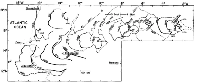
Sutton (1925) characterized haboobs in the Sudan, where he observed haboobs with height of 1000 m or more and occurring commonly from May to October and noted that their passing was associated with a temperature drop. The haboobs he observed generally appeared to be small, strong, sand storms. Further study (Sutton, 1931) found that some, but not all haboobs were associated with precipitation — a more common event later in the rainy season than earlier — and about a third were associated with thunder or lightning, with the frequency of occurrence again increasing in later months. Sutton (1931) observed a diurnal cycle in haboobs seen at Khartoum, with a peak from 1800–2000 local time and a quiet period from 0400–1200 local time. In Section 5.1 we report observations that generally agree with Sutton except in one important way: he saw haboobs as purely local events with extent perhaps tens of kilometers, while we show evidence of dusty gust fronts whose extent is so large that it cannot be fully detected with ground-based radar.

The significant effect of haboobs on aviation makes it important to be able to pre-dict where they will appear and where they will go. An unexpected haboob disrupted

(19)

Figure 1-1: This photograph of a dusty gust front in Niamey, Niger was taken by Brian Russell. The photo shows a typical dusty gust front structure: a layer of dust, topped by a white section of cumulus cloud that results from lifting in the gust front updraft over the top of the dust layer.

(20)

the rescue of Iranian hostages in 1980 (Wilkerson, 1991), and the microbursts that create haboobs have been blamed for serious civil aviation accidents (Fujita, 1986) because their strong vertical wind shear is difficult to forecast.

In West Africa, isolated storms occur frequently throughout the summer. As a thunderstorm enters the mature stage, a downdraft develops, ultimately creating a microburst or downburst (Fujita, 1986) containing rain which, in the arid desert, evaporates before it hits the ground (Wilkerson, 1991). Evaporative cooling makes the downburst a gust of dry, cold air which entrains dust on the desert surface, creating a thin dusty gust front characterized by strong internal winds. The circumstances which create isolated thunderstorms frequently follow diurnal cycles (Janiga et al., 2009), which explains Sutton’s observations of a diurnal cycle in gust fronts at Khartoum and likewise matches our observations (Figure 5-2).

1.3 MCSs and squall lines

The circumstances that give rise to a single thunderstorm may also create a group of cells of strong, cold convective activity surrounded by cells of cells of moderate strength, which are initiated, propagate, and dissipate in an organized fashion col-lectively called a mesoscale convective system (MCS) (Machado et al., 1998). The distinction between an MCS and a single large thunderstorm or “supercell” is of-ten not clear in practice, especially when observations are made with low-resolution satellite images.

A particular kind of MCS common to West Africa is the squall line, an organized line of thunderstorms. These systems are characterized by a leading edge of convective cells typically hundreds of kilometers long but sometimes more than 1000 km long (Rowell and Milford , 1993). Anvil cloud extends behind this leading convection; the and is associated with additional, weaker rainfall that is called trailing stratiform precipitation. Squall lines are considered the most important convective systems in West Africa because they influence the movement of the monsoon front during the June-September rainy season and can themselves initiate new squall lines (Peters

(21)

Figure 1-2: This image, Figure 1 from Fortune (1980), shows the track of a single continuous system composed of multiple squall lines over 48 hours in September 1974. Compare with our Figure 4-1, which also shows the progression of fronts for a large, synoptic-scale system of squall lines.

and Tetzlaff , 1988) and because they contribute much of the total seasonal rainfall. Squall line generation is often influenced by the African Easterly Wave, especially at the West African coast (longitude 15W) and in the Sahel region (Fink and Reiner , 2003).

Fortune (Fortune, 1980) observed a single system composed of individual squall lines which themselves only propagated for 6-12 hours; however, he tracked a coher-ent “family” of these squall lines and other convection which propagated from 4–5 September 1974, moving for 48 hours over 2000 km as a series of curved squall line fronts (see Figure 1-2 for his graph of the squall line system’s evolution).

In Fortune (1980), a squall line system represents a mesoscale or synoptic-scale perturbation in the mid-level wind field. Many MCSs exist which cannot be explained using the simple squall line model but include additional forms of convection; these MCSs can propagate for long distances and initiate new convection, so they are me-teorologically significant. Within a squall line, the heavy rainfall of the leading edge is preceded by a well-marked gust fronts (Chong et al., 1987). These gust fronts, like

(22)

those generated from isolated thunderstorms, loft dust and create haboobs.

At the Niamey radar site, we observe gust fronts generated along squall lines and traveling within squall line systems as they travel for hundreds or thousands of kilometers. Most of the gust fronts we observed using satellite infrared imagery are associated with squall lines: although isolated thunderstorms outnumber squall lines in West African weather, squall lines travel further and are more likely to cross the Niamey site. Diurnal influence and local geography play lesser roles when squall lines cross our observation site because the squall lines last longer.

1.4 African Easterly waves

Long-lived seasonal perturbations in the mid-level wind field or in potential vorticity are the result of tropical waves, called African Easterly waves (Reed et al., 1977). They can contribute to mesoscale convective activity and are also thought to originate from localized forcing (Thorncroft et al., 2008). The strongest AEWs, associated with outgoing longwave radiation (OLR) signals that indicate deep convection (Kiladis et al., 2006), have phase speed about 11.5 m/s east of 0 E and slow down to about 8.5 m/s as they head west over the Atlantic Ocean; they had wavelengths of 3000– 3600 km, based on OLR measurements. Synoptic analysis of two main AEW tracks over West Africa at 5 N and 15 N found waves with period 3–5 days and 6–9 days and characterized the 6–9 day waves as more active in August–September than June–July, with mean wavelength 3000 km north of the African Easterly Jet (AEJ) and 5000 km south of the AEJ, and with mean phase speed 8 m/s north of the AEJ and 12 m/s south of the AEJ (Diedhiou et al., 1999). The typical AEW with period 3–5 days is characterized with wavelength 2000–4000 km and phase speed 6–8 m/s (Hsieh and Cook , 2005); within the single season August–September 1985, the 3–5 day period waves had wavelength 2500 km and phase speed 8 m/s (Reed et al., 1988).

There is not always an African Easterly wave over the continent, nor need there be only one — the troughs of multiple waves may be visible across the continent simultaneously. In 2006, organized wave behavior was particularly notable in late

(23)

August and throughout September (Janiga, 2010).

When squall lines are observed in the presence of an AEW, they typically form west of the trough (Peters and Tetzlaff , 1988) where northerly flow contributes vertical wind shear; when there is only a single wave on the continent and no trough to form west of, they may also develop in a secondary preferred region of development east of the ridge (Schrage et al., 2006), where southerly flow introduces moist air in moisture-scarce regions. The largest contribution of the AEW to MCSs may be to their formation: Peters and Tetzlaff observed a mean squall line speed of 16 m/s, faster than wind speeds inside the African Easterly Jet1_{, and remarked that these squall}

lines must be passing through the AEW, a comment shared by (Fortune, 1980) in a system which propagated about twice as fast as the AEW. We present an alternate theory in Section 5.8: long-lived squall line systems may be suppressed by an AEW, but they are nevertheless common occurrences in West Africa because of the frequent absence of a strong AEW obstructing squall line redevelopment. Bou Karam et al. (2010) showed another unusual situation where a squall line reaches the synoptic scale, and can even intensify an AEW, in a 3-6 August 2006 case where a thousand-kilometer arc of dust pushed across the continent and organized new convection along the front (Bou Karam et al., 2010).

1.5 Thesis structure

Chapter 2 describes the instruments used to measure the propagation and physical properties associated with gust fronts and MCSs.

Chapter 3 is a conceptual review of the literature behind how gust fronts are thought to form, propagate, and assist new convection; how the aerosol in dusty gust fronts affects the weather; how MCSs propagate; how how AEWs interact with MCSs. Chapter 4 explains the techniques used to turn the raw data described in Chapter 2 into processed values. We discuss how we generated gust front speed, propagation

1_{In “dry” and “realistic” simulations, the AEJ had maximum wind speed of 15 m/s in the west}

coast of Africa; in “wet” simulations, the AEJ had maximum zonal wind speed of 9 m/s(Hsieh and Cook, 2005).

(24)

distance, and duration, as measured by radar and satellite imagery; we show how to generate Hovmoller diagrams that depict the long-term movement of features identi-fied in lightning strike data; and we describe the Lagrangian method used to quantify how much lightning is associated with an event.

Chapter 5 presents the key results of the thesis. It includes a tabulation of all observed gust fronts and a discussion of their diurnal and geographic frequency; an observational test of gust front speed and temperature drop that validates the density-current model; evidence for the conceptual model of gust front initiation in the form of Lagrangian lightning counts that show a way for us to quantify a storm’s convective strength; and a large mean extent for satellite-observed gust fronts of 750 km. Finally, we discuss an intriguing phenomenon that appears in a diagram showing long-term lightning behavior: long, continuous “stripes” of convection as long as an African Easterly wavelength and twice as fast.

Chapter 6 concludes with a discussion of our contributions to the study of gust fronts and MCSs.

(25)

Chapter 2 Apparatus

This chapter discusses the devices used to measure the propagation and physical prop-erties associated with gust fronts and mesoscale convective systems (MCSs). These apparatus include radar, satellite infrared sensors, surface meteorology instruments, and specially equipped radio receivers.

2.1 MIT Doppler Radar

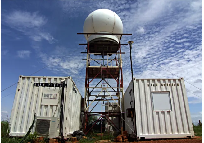
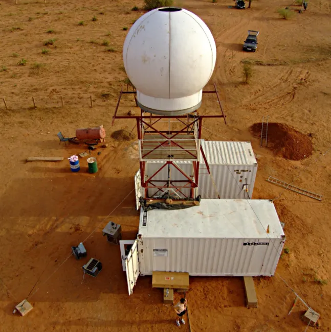
A C-band (λ = 5.30 cm) Doppler radar used by the MIT Weather Radar Labora-tory (Russell et al., 2010) was operated from 5 July–27 September 2006 with lowest elevation angle 0.7 degrees and maximum recorded range 250 km in Niamey, Niger (13.4915 N, 2.1698 E, 224 m altitude) (Chong, 2009). See photographs of the instal-lation, Figures 2-1 and 2-2.

Russell et al. (2010) gives a concise but thorough history of the device, dubbed the MIT WR-73 weather radar, which has seen wide use since its acquisition in the 1970s for use by the MIT Weather Radar Laboratory and operated aboard the R/V Gilliss during the Global Atlantic Tropical Experiment (GATE) (Geotis, 1978).

It has since traveled the globe; among the locations Russell et al. mentions are Borneo for the International Winter Monsoon Experiment (WMONEX) (Houze Jr et al., 1981), North Carolina for the Genesis of Atlantic Lows Experiment (GALE) (Engholm et al., 1990), Darwin, Australia for the Down Under Doppler and

(26)

Electric-Figure 2-1: The MIT radar installation at Niamey. Photograph taken 16 September 2006 by Brian Russell.

(27)

Figure 2-2: A photograph of the MIT radar installation at Niamey from the tower over the radar. Photograph taken 12 September 2006 by Brian Russell.

(28)

ity Experiment (DUNDEE) (Rutledge et al., 1992), aboard R/V John V. Vickers off the coast of Papua New Guinea for the Tropical Ocean Global Atmospheres/Coupled Ocean Atmosphere Response Experiment (TOGA COARE) (Rickenbach and Rut-ledge, 1998), aboard R/V Ronald H. Brown in the middle of the Pacific Ocean about halfway between Hawaii and Ecuador for the Pan-American Climate Study (PACS) (Yuter and Houze, 2000), and in Alabama for microburst detection studies (Williams et al., 1989). When not otherwise engaged, the MIT radar sits atop the Green Build-ing.

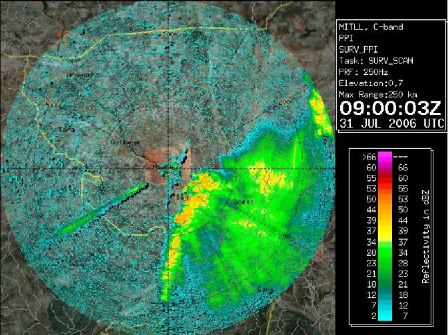
Radar surveillance scans were recorded every 10 minutes. Of 40 gust fronts iden-tified crossing the Niamey radar site in June–September 2006, 32 crossed while the radar was operational, and radar PPI images show 22 of those gust fronts crossing the Niamey site. The other 10 fronts are not documented only because not every surveillance scan was readily available; in every case where a surveillance scan was available and a gust front was observed, it was visible on the radar.

It is straightforward to locate fronts (though they are sometimes delicate) and the reflectivity signature associated with convection, with one important caveat: reflec-tions off a large aircraft hangar create a phantom line that looks like convection in the southwest quadrant (see for example Figure 2-3, a surveillance scan showing the phantom line).

The curvature of the Earth, combined with the low height of a gust front’s head (its radar-detectable features have a ceiling around 2 km) and the elevation angle of the radar imply a maximum radius of less than 80 km for detection of gust fronts.

Scans available for 1–2 July and 4–5 July were made with elevation angle 0.5 degrees and maximum recorded range 150 km. The lower elevation angle implies a lower beam bottom, so the radar should be able to detect gust fronts at slightly greater distances for those two scans.

(29)

Figure 2-3: This radar surveillance scan for 31 July 2006 at 0900 UTC shows a gust front just east of the MIT radar site and the phantom line southwest of the radar site, caused by reflection off a large aircraft hangar nearby.

(30)

2.2 SEVIRI satellite imagery

The European Organisation for the Exploitation of Meteorological Satellites (EU-METSAT) operates two independent Meteosat Second Generation weather satellites in geostationary orbit around the Earth at approximately 0 degrees east, 0 degrees north (Schmetz et al., 2002).

The satellites carry several instruments, including a radiometer called the Spinning Enhanced Visible and Infrared Imager (SEVIRI) with 12 channels that record 10-bit pixels in twelve image channels, ranging from 0.4µm–13.4µm. High-resolution (3 km) SEVIRI images of Europe, the North Atlantic, and Africa are made available at 15-minute intervals. The visible-to-infrared scale of the sensors allows the detection of shallow features with more precision than older satellite data products allowed.

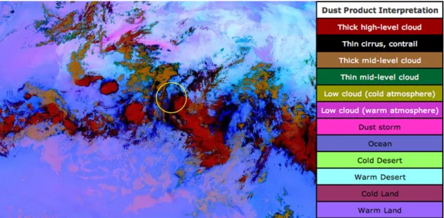
Among EUMETSAT’s data products is an RGB composite dust product, calcu-lated based on three SEVIRI infrared channels and capable of revealing the transport of large amounts of lofted dust. In this product, the blue channel is created from the SEVIRI 10.8µm image, and the red and green channels are created by subtraction: red is 12µm - 10.8µm and green is 10.8µm - 8.7µm1. More sophisticated dust prod-ucts that take advantage of information about the microphysics of dust are widely available (Lensky and Rosenfeld , 2008), but we elected to use the simple SEVIRI data product and found it highly effective in detecting dust movement associated with gust fronts. We sometimes found it helpful to examine only the green channel, which pro-duces sharp boundaries along the edge of events but lacks the RGB product’s power in qualitatively distinguishing dust from cloud and other IR-detected features.

The standard SEVIRI dust product is a “full-disc” image (see Figure 2-4) covering all of Europe and Africa and much of South America. This region is much larger than is interesting for our study of events in West Africa. We use an archive of these dust images as provided by the RADAGAST project (Miller and Slingo, 2007) and constrained to the region from 25 W to 25 E and 5 S to 30 N. Figure 2-5 shows one sample image of the SEVIRI dust product used for this research. The process

(31)

used to transform these geostationary-projection images into rectilinear coordinates is documented in Section 4.5.

2.3 ZEUS/STARNET VLF lightning network

The ZEUS/STARNET lightning network (Chronis et al., 2004) is an integration of radio receivers in Africa, Europe, and the Americas (Morales and Anagnostou, 2003) listening within the VLF range (specifically at 7–15 kHz) to measure the atmospheric radiation effects of lightning strikes. Atmospheric radiation pulses from lightning (sferics), primarily from the return strikes of cloud-to-ground flashes, can be triangu-lated using a technique traditionally called Arrival Time Distance (ATD), creating a long-range lightning network that can reliably locate lightning strikes in West Africa. With the ATD method, receivers have GPS-synchronized clocks and record the ar-rival time of sferics; when an event is detected by multiple receivers, those receivers’ known location and the difference between arrival time creates a set of possible points and times where the lightning could have struck. A single event is detected in mul-tiple receivers, creating many sets of data that can be intersected (or, equivalently, equations that can be solved) to find the lightning strike in space and time.

The number of active receivers in the ZEUS/STARNET network is ever chang-ing. From 25 July–30 September 2006, “European” ZEUS receivers were active in Birmingham, U.K.; Roskilde, Denmark; Iasi, Romania; Larnaka, Cyprus; and Evora, Portugal; and “African” STARNET receivers were active in Adis Ababa, Ethiopia; Dar es Salaam, Tanzania; Bethlehem, South Africa; and Osun state, Nige-ria. The location of events in 2006 also used additional Western-Hemisphere re-ceivers, including sites in Guadeloupe; Fortaleza, Brazil; and Sao Paulo, Brazil. Re-processed data are available for a slightly shorter interval, from 1 August–30 Septem-ber 2006. The full network recorded 18.4 million strikes for August 2006 and 34 million strikes in September 2006. The complete data set is available online at http : //www.zeus.iag.usp.br/AM M A/f tp/tar/ but remains provisional and subject to additional reprocessing (Morales, 2010); with additional preprocessing to include

(32)

Figure 2-4: The SEVIRI 10.8µm “full disc” image from 17 May 2010 at 2000 UTC for 30 August 2006 at 0730. The A circle is shown with radius approximately 250km and centered over Niamey, the same bounds shown in our radar PPI images

(33)

Figure 2-5: The SEVIRI dust product for 30 August 2006 at 0730. A circle is shown with radius approximately 250km and centered over Niamey, the same bounds shown in our radar PPI images

only strikes with less than 20 microseconds of residual error in the ATD solution (a method Morales (2010) recommends), we obtained useful data.

The time error of these data is reportedly on the order of 1 millisecond. The spatial error of these data is reportedly 10–20 km within the network, so they are especially useful in the aggregate for tracking events that generate substantial num-bers of lightning strikes, like MCSs and squall lines. This reported error is consistent with an error analysis of the ZEUS network in 2003 when it consisted of six receivers throughout Europe (Chronis and Anagnostou, 2003); its error was found to be less than 40 km within the network (mode 20) and less than 400 km (mode 220 km) for locations > 5000 km outside the network The convective environment around Niger is within a few hundred kilometers of the monitoring station at Osun, Nigeria and surrounded by other stations, so we should expect to see low, in-network spatial error for all lightning measurements we use. We overlaid these lightning strikes on top of SEVIRI dust product images (Section 4.5) and found that the two generally agreed; the lightning strikes plotted in aggregate appear to show squall lines, MCSs, and isolated thunderstorms atop those features as detected in SEVIRI dust product data. The lightning data include a few unusual features, such as a tendency to show a sharp

(34)

diagonal line of strikes along a front which overshoots the actual front boundary as shown in previous and subsequent lightning and dust product images; so it is helpful to compare them with satellite images. Likewise, the satellite images sometimes show apparent strong cloud activity and dust movement which actually has few correspond-ing lightncorrespond-ing strikes; lightncorrespond-ing strike data enhances our understandcorrespond-ing of exactly when convection regenerates along a gust front and when a storm has dissipated most of its convective energy, but its associated cloud continues to move.

2.4 ARM Mobile Facility surface meteorological

station

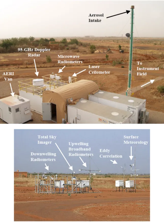
We use one-minute-resolution data from the surface meteorological instrumentation of the Atmospheric Radiation Program Mobile Facility (Ackerman and Stokes, 2003) deployed in Niamey in 2006 to coincide with the African Monsoon Multidisciplinary Analysis (AMMA) (Redelsperger et al., 2006). Data from ARM (see installation photographs, Figure 2-6) and AMMA have helped focus attention on Saharan dust storms, where surface stations provide information about the dust’s optical proper-ties and its contribution to radiation balance that cannot be inferred from satellite information alone (Slingo et al., 2006). The ARM Mobile Facility’s high-frequency samples of basic surface station measurements — visibility, wind speed and direction, temperature, moisture, and rainfall — provide key data that have greatly improved our understanding of gust front behavior. The instruments do, however, represent only a point sample, so their measurements may not be complete representations of conditions all along a front.

Wakimoto (1982) found that as gust fronts at mid-latitude crossed a surface sta-tion, meteorological instruments recorded a pressure rise, followed by a wind shift, then a wind surge, a temperature drop, and finally rainfall. Figure 5-14, a plot of ARM Mobile Facility instrument data from 11 July 2006, shows a sample case that validates this pattern. The data available from the ARM site are extravagant in

(35)

Figure 2-6: Top: the Atmospheric Radiation Program Mobile Facility in Niamey, Niger. Bottom: the associated instrument field, approximately 100 m from the main facility. Photos from Sally McFarlane and attributed to Mark Miller.

(36)

their reliability, high 1-minute sampling rate, and availability of corroborating data from additional sensors. However, the quantities they measure are basic enough that gust front signatures can be sought among data from other surface stations in Africa, for example one-hour resolution data widely available in surface stations throughout the continent. We have documented evidence of a particular gust front studied by Bou Karam et al. (2010) using surface station data from Agadez, Niger; In Salah, Algeria; and Tamanrasset, Algeria.

2.5 ECMWF vorticity analysis

The European Centre for Medium-Range Weather Forecasts provides daily global analyses and reanalyses at 0000, 0600, 1200, and 1800 UTC that forecast common atmospheric factors including wind and temperature. To understand MCS interac-tion with synoptic-scale African Easterly waves, we have relied on the interpretainterac-tion of another ECMWF data product, the interim reanalysis, which provides potential vorticity at 700 hPa at 1.5 degree resolution. (Vorticity measures the rotation of the air at that altitude relative to the Earth’s surface, with a positive vorticity meaning clockwise motion.)

2.6 CALIPSO satellite lidar

NASA’s Cloud-Aerosol Lidar and Infrared Pathfinder Satellite Observation mission (CALIPSO) carries three instruments: the 532 nm and 1064 nm Cloud-Aerosol Lidar with Orthogonal Polarization (CALIOP) (Winker et al., 2007), the Imaging Infrared Radiometer (IIR), and the Wide Field Camera (WFC). CALIPSO and the CloudSat satellite (which measures clouds with a W-band radar) were integrated in April 2006 into a formation of three other satellites, collectively called the “A-Train”, which fly along a 705 km sun-synchronous orbit and cross the equator at 1330 local time (McGill et al., 2007). The same location on the ground is measured by each satellite within a 15-minute interval, and CALIPSO and CloudSat are kept within 15 seconds

(37)

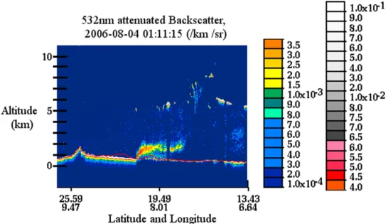
Figure 2-7: The CALIPSO lidar image of a gust front on 4 August 2006, as reported in Bou Karam et al. (2010), shows a gust front with a head approximately 2 km high.

of one another.

Attempts to locate intersections of gust fronts with CALIPSO lidar were largely unsuccessful, in part because the CALIPSO lidar’s observation grid covers a different vertical track every few days, reducing the number of times where an intersection is possible, and in part because gust fronts are narrow features oriented mostly north-to-south, and the lidar track is also narrow and oriented north-to-south. Intersections with a synoptic-scale event with a gust front oriented west-to-east were successfully located in Bou Karam et al. (2010). The relevant portion of the CALIPSO track is reproduced in Figure 2-7, showing a 2 km height for the gust front’s head.

Our research has shown a way to identify gust fronts’ precise location as they are launched and propagate across Africa using geostationary satellite imagery. This improved view of gust front location and propagation distance means that future attempts to find CALIPSO intersections with gust fronts are likely to be substantially more successful than attempts to locate intersections using spatially restricted radar data alone.

(38)

(39)

Chapter 3 Conceptual background

This chapter introduces the concepts behind how gust fronts are thought to form, propagate, and assist new convection; how the aerosol in dusty gust fronts affects the weather; how mesoscale convective systems (MCSs) propagate; and how African Easterly waves (AEWs) interact with MCSs.

3.1 Gust front initiation

The Thunderstorm Project (Byers and Braham, 1949) identified three phases of a thunderstorm: the cumulus stage, typified by an updraft of air traveling about 1–30 m/s as clouds grow and accumulate water, and drops begin to fall; the mature stage, in which the updraft continues but is adjoined by a downdraft caused by evaporative cooling when massive water droplets and graupel particles drag air downward; and the dissipating stage, in which air flows predominantly downward until the cloud breaks up.

As a thunderstorm enters the mature stage, the initial downdraft cools down relatively slowly, and mixture with outside air results in evaporative cooling that keeps the downdraft cold relative to its surroundings. An outflow of cold air is thus directly associated with the downdraft. When the outflow is associated with strong winds, a persistent discontinuity forms between the outflow and the surrounding air; this outflow boundary outruns the rain and is detected miles beyond the periphery

(40)

of the storm cell. Byers (1949) reported that the first gust of air from a downburst is the strongest (a view confirmed by the laboratory models of Fujita et al. (1990)). They propose that strong winds continue to be associated with the cold outflow, with the wind speed and “gustiness” decreasing as the air spreads farther away. They add a caveat that the gust front’s wind speed may be sustained if a nearby cell reaches the mature stage and releases a new burst of cold air to sustain the existing gust front. This is the case for a row of thunderstorms making up a squall line, where each new convective cell provides more cold air to a cold pool. If each thunderstorm experiences a downdraft and launches a gust front in concert, a one-dimensional gust front is launched parallel to the parent squall line.

3.2 Gust front propagation

A gust front can be modeled physically as a density current, sometimes called a gravity current, an event where a density contrast exists between two fluids (in this case, between the cold, moist front and the warm, dry surroundings) (Simpson, 1982). The current is sustained as the warm air rises above the head of the current to produce mixing billows. The shape of a dusty gust front, or haboob, has been found to match closely with the shape of laboratory models of density currents made by introducing salt into fresh water (Simpson, 1969). A single gust front was examined by Charba (1974), who found that its structural characteristics (head at 1700 m, cold air with constant depth 3350 m upstream of the head, wind speed surge slowed at the ground by frictional drag, large vertical wind shear at front edge) showed much similarity with laboratory simulations.

Knippertz et al. (2009) conducted numerical simulations of three gust fronts, treated as density currents, and performed sensitivity studies to show that the posi-tion and propagaposi-tion direcposi-tion of a density current depends largely on the initiaposi-tion parameters of deep convective cells; that is to say, the problem forecasting gust fronts was found to be essentially a problem of forecasting moist convection. One microphys-ical result of the sensitivity study did affect gust front speed: when the turbulence

(41)

length used for vertical mixing was increased, precipitation was more common but weaker, and the gust front was reportedly larger and faster, with higher winds. The theoretical density current propagation speed, for incompressible steady flows, is of-ten given as Vf = k(gH∆ρ/ρ)1/2 (Droegemeier and Wilhelmson, 1987) and depends

on g, acceleration due to gravity; k, internal Froude number; ∆ρ, the contrast in air of a density current across the front; ρ, the density of the environment; H, the height of the density current head or of the cold air upstream of the head. Numerical models based on this relationship found that gust front head depth and propagation speed depended primarily on the outflow’s vertical temperature distribution (explain-ing why in atmospheric tests, the ratio ∆ρ/ρ is sometimes replaced by ∆T /T ). A similar equation proposed by Wakimoto (1982) is tested in Section 5.4.3.

Traditional models of gust fronts as density currents are one-dimensional; the gust front propagates “forwards” and the squall line is “behind” the gust front. In satel-lite observations of two-dimensional gust fronts which form as circular outflows from isolated thunderstorms, we observe these fronts propagating quickly after the initial outflow, then slowing down. The behavior of two-dimensional outflows has been stud-ied in the context of viscous fluid dynamics: Simpson (1987) (citing (Huppert (1982) and Didden and Maxworthy (1982)) distinguishes between “radial” (one-dimensional) and “two-dimensional” gravity currents. For the radial case, velocity and time are related V ∼ t−7/8, while the relationship for the two-dimensional case is V ∼ t−1/5. These theoretical results, although designed for a viscous model, are consistent with our qualitative observation that gust front velocity declines over time more quickly for isolated thunderstorm outflows compared with outflows from squall lines.

3.3 Gust front-initiated convection

The analysis of thermodynamic soundings (Williams and Renno, 1993) has shown that much of the tropical atmosphere is conditionally unstable. In many situations, a finite vertical displacement of a surface parcel is sufficient to release the instability and create moist convection.

(42)

Wilson and Schreiber (1986) found that most new storms form near a boundary like a gust front and that boundaries are associated with the resurgence of old storms, with storms very likely to form within 0–20 km of a moving boundary, within 15 km of a stationary boundary, and within 5 km of colliding boundaries. They theorized that when boundaries collide, forced lifting intensifies, making new convection easier to form. In their study, colliding boundaries which created new atmospheric instability, as measured by comparing condensation temperature versus sounding temperature, were most likely to create new convection or strengthen existing convection.

Regeneration of convection along a single squall line was modeled by Crook et al. (1990), a study which found three characteristics in the regeneration: an increase in low-level moisture; an increase in low-level shear; and a mesoscale oscillation, or “sloshing”, in which a convective system’s subsidence stage feeds the formation of a new convective system along the first system’s gust front. Even when a storm is convectively inactive, the gust front still forces velocity on the order of 6–7 m/s, a factor Crook et al. (1990) deliberately excluded from models to isolate the mesoscale oscillation effect. This effect was explained as the atmospheric response to the heating and cooling of the convective system.

An analysis of 30 gust fronts with average head depth 1.3 km, average temper-ature drop 3.5 C, and average propagation speed 8.6 m/s (Mahoney, 1988) found that outflow boundaries can create new convection by mechanical forcing, or by a mechanism that makes strong updrafts, extending higher than boundary layer tops, and creates circulation that gives rise to new convection. Curiously, the gust front speeds recorded by Mahoney do not correlate well with measured temperature drop, as we found with ARM data (Figure 5-19 in Section 5.4.3).

3.4 Characteristics of dusty events

Not all gust fronts are dusty. Gust fronts at mid-latitude propagating over vegetated terrain are nearly invisible. But nearly all gust fronts over the semi-arid Sahel and the arid Sahara are prominently dusty. Vertical dust flux is related by a cubic function

(43)

to wind speed (Cakmur et al., 2004), and the strong vertical wind shear associated with gust fronts lofts large amounts of dust.

Whether gusty dust fronts affect convection differently, and the specific effect of dust, can be understood as a case of the general problem of the effect of aerosol par-ticles on convection, a question which is especially timely for global climate models. Qualitatively, increasing aerosol concentration results in more cloud condensation nuclei, a key factor in the microphysics of convection. But the literature is con-flicted on what, exactly, those extra CCN do — in Rosenfeld (1999), smoke from forest fires almost completely suppressed tropical warm rain processes, and air pollu-tion was found to suppress rainfall in extra-tropical locapollu-tions. Subsequent numerical modeling (Khain and Pokrovsky, 2004) reproduced this result, showing that under cloud-dynamics models, high aerosol concentrations will increase the height at which rainfall begins. Fan et al. (2007) used simulations to create the more nuanced hypoth-esis that aerosol has minimal effects on cloud microphysics for dry air (40% surface relative humidity), but in moist conditions (60–70% surface RH), increases in aerosol concentration will increase cloud water content and create stronger precipitation and more intense radar reflectivity within convective systems.

Local storms loft significant amounts of dust and can contribute to the dustiness of West Africa far from the initial convection; in a 7–8 July 2006 case (Bou Karam et al., 2009), a dry cyclone that formed over Niger created strong surface winds of about 11 m/s and lofted substantial amounts of dust to 4–5 km altitude, where it was available for long-range transport over distances far exceeding the cyclone’s 400 km width.

Other effects of African dust on weather have been noted by Anuforom (2007), who remarked that Saharan dust has been shown to affect radiative balance (Diaz et al., 2001) and atmospheric electrical properties (Ette, 1971) (also studied recently in the Sahel by Williams et al. (2009)). Flamant et al. (2009) studied a 5–6 June 2006 case and found that large amounts of dust in a gust front affect not just the cloud, but also the insolation in the region of the Sahelo-Saharan planetary boundary layer, affecting the development of the intertropical discontinuity (ITD), the movement of

(44)

which is a key synoptic-scale driver for the rainfall of the monsoon season.

3.5 MCS behavior with size

Satellite analysis of the cloud associated with 3200 deep convective systems (regions with satellite infrared temperature TIR= 245K or lower) by a tropical meteorologist

and 4700 by an automated system found that the average radius of the MCS is linearly correlated with the average lifetime (Machado et al., 1998); the results were the same for the manually and automatically tracked systems, although the reported average size of an MCS was 20–30% higher for the automatically tracked MCSs, suggesting sensitivity issues in the process. The larger systems were found to have larger system-average reflectance and more, larger, colder convective clusters (highly active, cold TIR ¡ 218 K, centers of convection). Larger system reflectance was correlated with

system lifetime, a result which supports the measurements of Mathon and Laurent (2001) that larger MCSs have longer lifetimes.

Rotunno et al. (1988) discussed the theoretical underpinnings for how MCSs inter-act to form squall lines and provided a theory showing how independent, moderately sized cells of MCSs could interact without any need for a “special” kind of squall line MCS.

The observations discussed in Section 5.6 cast doubt on the idea that squall line MCS (SLMCS) speed increases with size, but evidence is also presented that SLMCS lifetime, propagation distance, and total lightning production all increase notably with size.

3.6 AEW interaction with

squall line mesoscale convective systems

The propagation of AEWs is important to forecasters because there is a relationship between more AEWs leaving the African coast and a more intense Atlantic tropical cyclone season (Thorncroft and Hodges, 2001). An AEW can be triggered by

(45)

con-vection that generates a MCS, as in Berry and Thorncroft (2005), a case study of an AEW in 2000 which was likely triggered by an MCS but which also triggered multiple new MCSs within the AEW’s structure.

Strong convective systems are often triggered by strong shear in the African East-erly Jet (Mohr and Thorncroft , 2006), the same phenomenon which contains instabil-ities that give rise to AEWs. Simulations of the AEW and AEJ show that moist con-vection can reinvigorate AEWs, contributing to their development (Cornforth et al., 2009). Understanding how and where MCSs form and propagate can thus improve our understanding of AEW behavior.

AEWs have long been thought to constrain the development and westward prop-agation of individual MCSs: in Reed et al. (1988) squall lines are shown to grow east of an AEW’s ridge and die near an AEW’s trough. According to this view, an MCS generated within an AEW is halted within that AEW. In Payne and McGarry (1977, Figure 10), convective cloud is shown to vary in quantity depending on its proximity to an AEW. Recent work by Fink and Reiner (2003) examining West Africa in 1998 and 1999 found a favorable location for squall line generation in the area west of the AEW trough (which, because of the nature of an AEW nature, is roughly equivalent to the area east of the ridge). That study showed a stronger influence of the AEW the further west it was located: AEWs contributed to 20% of squall line generation at 15 E and 68% of squall line generation at 15 W. The relationship between AEW and squall line organization was found to be strongest in August and September.

We show in Section 5.8 that SLMCSs in August and September 2006 that prop-agate distances substantially greater than half a typical AEW wavelength can do so because no prominent AEW is present.

(46)

(47)

Chapter 4 Processing sensor data

This chapter discusses the techniques used to turn the raw data from our apparatus into processed values. We discuss how we generated gust front speed, propagation distance, and duration, as measured by radar and satellite imagery; we show how to generate Hovmoller diagrams that depict the long-term movement of features identi-fied in lightning strike data; and we describe the Lagrangian method used to quantify how much lightning is associated with an event.

4.1 Determining GF speed from radar images

4.1.1 Tracking gust fronts

Each individual image frame from the 10-minute radar surveillance scans containing a gust front was annotated with the location of the front, and the front’s travel was tracked with “CellTracker” software, originally designed for tracking the movement of biological cells in microscopy (Shen et al., 2006). Multiple tracks were annotated along different points of the radar-visible front, then a single track was created which represented the part of the front that crossed the radar site (generally the center of the visible portion) and traveled perpendicularly between each front as defined every 10 minutes. This averaging provides a better accounting for local variation in front propagation than simply using a single track. We also tried computing

(48)

the area between the fronts and dividing by the average linear extent (based on the track measurements), but the calculation turned out to be unreliably sensitive to how much of the front was visible. We use the distance traveled along a track immediately before crossing the MIT radar site and immediately after, divided by 10 minutes, as an “instantaneous” speed associated with the radar crossing.

4.1.2 Errors in gust front speeds

Most of the MIT radar PPI images had resolution of 500 km / 480 px, meaning that an error of one pixel in a ten minute interval results in an error of 1.73 m/s in speed. (Two early scans in July had resolution 300 km / 480 px instead, so a one-pixel difference in ten minutes is a difference of 1.04 m/s in speed for those events.)

The manual process used to annotate tracks was performed by rigorously measur-ing gust fronts that extended for tens of pixels, so the actual error of the change in front movement has error at the sub-pixel scale, less than 1.73 m/s. In some frames more distant from the radar, the front cannot be seen well, and error may be higher (we infer the front’s position when we can see it in frame 1 and 3 but not 2, for ex-ample). It is easiest to see thin lines when they’re directly over the radar site, which means that the instantaneous speeds we report are the most accurate of any of the 10-minute speeds we recorded.

4.1.3 Propagation distances and times for gust fronts

This calculation also produced gust front propagation distances and times, which, owing to the limited horizontal resolution of the radar for low features, were quite short. For events where radar data was available and the gust front could be clearly measured, it had measurable extents from 4 to 18 frames, with a mean of 9.5, corre-sponding to being detectable in radar for 40 to 180 minutes, with a mean of just 95 minutes.

(49)

4.2 Determining squall line speed

4.2.1 Radar image processing

Rickenbach et al. (2009) analyzed a complete collection of MIT radar volumetric images from 5 July-27 September 2006 by manually tracking the leading edge of squall lines in successive images. Their work focuses on “squall line MCSs”, the MCSs composed of a single strong squall line, which represent the most common type of MCS at Niamey from July-September. They produced speed information for 28 of those squall lines.

4.3 Determining gust front speed

from satellite images

4.3.1 Manual annotation

The same manual annotation approach that generates speeds for radar images can be applied to SEVIRI satellite dust product imagery. Because the resolution of the images is lower, the stakes are higher: we use RADAGAST project images with 6.3 km/pixel resolution, for which a single pixel error in a 15 minute interval represents a difference in speed of 7 m/s. By limiting our measurements to change per 3 hours, we reduce error to 0.58 m/s per pixel. Our actual measurements were performed along events visible in tens or hundreds of pixels and were performed with enough rigor to ensure sub-pixel precision. This method works well only for dusty gust fronts with a large extent, hundreds of kilometers or more, whose progress can easily be tracked with relatively low-resolution images. Small gust fronts from moderately sized MCSs may appear as only a few pixels in SEVIRI images, at least initially. On the other hand, large fronts may vary substantially in behavior along local subsections of the front, and those variations can make it difficult to track the exact location of a large gust front.

(50)

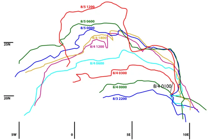
Figure 4-1: The track of the dusty gust front associated with a synoptic-scale event from 3-5 August 2006, propagating northward through West Africa. The gray line marked “8/4 0100” drawn perpendicular to the front between 5 E and 10 E is the intersection of CALIPSO satellite lidar with the front, shown in Figure 2-7 and dis-cussed in Bou Karam et al. (2010).

a synoptic-scale event from 3-5 August 2006 (Bou Karam et al., 2010), one headed north and the other headed west through Niamey, by applying a contrast-enhancing filter to the image, then manually creating a vector graphic that traced the front’s edge exactly. We overlaid the individual tracks of the northward event to create Figure 4-1, which shows that this method is viable for tracking the motion of synoptic-scale events. The measured edges of the fronts change from image to image as the dusty gust front becomes more or less readily discerned from surroundings. The technique’s key disadvantages is that it works well only for large events.

(51)

4.3.2 Automated measurements

To reduce error, we had to limit sampling to only every three or six hours. But this method seems to discard a disappointing amount of our 15-minute-resolution data. Luckily there is a solution: because we are more interested in the progress of fronts over time, we can use a method which discards almost all of the data at irrelevant locations and takes a cross section of the imagery along one possible track. This approach has been used when the actual track of an aircraft following a storm front was available (Flamant et al., 2007) But we show how it can be used when a precise track of the storm is not already known, by using two possible tracks, one which stays at Niamey’s latitude (13 N) and travels from east to west, and a second which stays at Niamey’s longitude (2E) and travels from north to south. Since most of the gust fronts we study cross Niamey traveling predominantly east-to-west (with a few propagating north-to-south), this simple approach is effective.

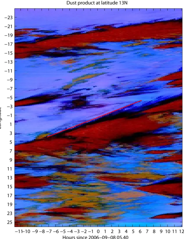
A sample dust product cross-section is shown in Figure 4-2. The front can be tracked as it crosses 13 N and heads west over time. A false-color version of the green channel alone (Figure 4-3) shows the change even more clearly. We can mark the beginning and end of a dust product in one of these cross-sections to find its distance traveled (in degrees latitude or longitude, which are roughly 111 km in extent near 0 N, 0 E) and the total time involved. By computing the slope, we can measure the gust front’s average speed over its entire detectable extent.

These cross-sections are effective at showing a front’s movement but may be mis-leading if a front leaves 13 N or 2 E completely, so we additionally use these measure-ments to produce more careful estimates. Manual examination of the SEVIRI dust product images around the observed beginning and end times from a cross-section image lets us locate the precise latitude, longitude, origin time, and ending time for each gust front that crossed the MIT radar.

(52)

Figure 4-2: In this typical SEVIRI dust product cross-section, a gust front that crossed the MIT radar site (longitude 2 E) on 8 September 2006 at 0540 UTC is tracked in SEVIRI dust product imagery for the 12 hours before and after the crossing.

(53)

Figure 4-3: This false-colored version of the green channel of Figure 4-2 shows the stark contrast of the front edge, also detectable in individual SEVIRI dust product image frames. Some space-time variability is evident along the leading edge of the front.

(54)

4.4 Stripes in the lightning Hovmoller diagram

4.4.1 Automated Hovmoller analysis

Hovmoller diagrams plot a scalar field’s value against time and one dimension of space and are helpful in meteorology for showing long-term phenomena where wave motion is suspected. The remaining dimensions of space not represented along one of the graphs’s axes are typically represented by integration. A concrete example is shown in Figure 4-4: we integrate lightning flashes from 8N–18N (a 10 degree latitude region centered on Niamey) and plot every day against longitude. This plot shows squall line MCSs as bands of lightning moving from east to west over many days. Each “cell” in this graph is an integration over 1 hour of time and one degree of longitude. (We generally graph only five or six days at a time and increase our time resolution to fifteen minutes per cell when we do so.) The Matlab code to generate these diagrams is given in Appendix A.1.

We plot the logarithm of lightning strikes per “cell”, a technique suggested by Morales (2010). Plotting a linear function of lightning strikes per cell results in muddy, hard-to-read images; plotting the logarithm of lightning strikes makes trends easier to see at the expense of making it difficult to check a specific numerical value — for example, values of 2000 and 3000 strikes per 15 minutes and per degree longitude are not readily distinguishable.

An especially interesting feature of these Hovmoller plots is the long, narrow stripes that represent squall lines, which we have quantified, characterized, and as-sociated with the translation of squall lines (see Section 5.7). These stripes typically have fairly constant slope (representing speed) throughout their propagation across the continent; their duration is typically several days; and their extent is tens of de-grees longitude. Occasionally a strong lightning storm spills into multiple Hovmoller cells, creating multiple possible “starts” or “ends”; at a time where lightning is active in multiple longitudes, we favor the westmost longitude for both “start” and “end” (this could represent the leading edge of a squall line), and at a longitude where lightning is active at multiple times we favor the earliest time for both “start” and

(55)

Figure 4-4: This lightning Hovmoller diagram shows lightning strikes for September 2006 integrated from 8-18 N latitude. Each distinct image cell has dimensions 1 degree longitude by 1 hour. Circled in white at 2 E longitude are the times when gust fronts were observed to cross the MIT radar at Niamey. A Hovmoller plot for August lightning activity is given in Figure 5-41.

(56)

“end” (a convention to make measurement consistent). Stripes sometimes include periods where there is little lightning activity; a stripe may include several segments separated by little or no lightning if the speed of each segment is nearly the same and the stripe exhibits continuity, such that there is no phase shift between the two segments.

A difference of a single cell in measuring distance represents 1 degree longitude (about 111 km); in measuring time it represents 15 minutes. The amount of error in our average speed calculations depends on the error in distance and time; for typical values of distance and time, an error of one “cell” in distance has an order of magnitude greater effect on speed than an error of one “cell” in time. For example, for a stripe with length 35 degrees longitude and duration 3 days, an error of 1 degree longitude would affect speed by about 0.4 m/s, and an error of 15 minutes would affect speed by about 0.05 m/s. We are measuring events along long lines, tens or hundreds of pixels in length, and so we likely encounter <1 pixel error.

4.5 Combining lightning maps and

SEVIRI infrared dust images

To improve the utility of the lightning stripes, we annotated each available SEVIRI dust product image frame with dots representing ZEUS/STARNET lightning strikes (see Section 2.3), then made movies showing the progress of storms as viewed by the dust product and lightning simultaneously throughout August and September. SEVIRI dust product images are available every 15 minutes and were annotated with the lightning data from the nearest 15 minutes (so an image from 0000 UTC was annotated with data from 2352:30–0007:30 UTC).

SEVIRI dust product images use a geostationary projection which becomes less linear the further the image is from 0 N, 0 E. The difference between the geostationary satellite projection and an equirectangular projection (linear relationship between latitude / longitude and pixel value) is minimal at Niamey and near the equator, but

(57)

above 20N it becomes especially noticeable. Although the SEVIRI image extends from 25W to 25E and 5S to 30N, at the top the image extends from (30.7 N, 30.3 W) to (30.7 N, 30.3 E), and at the bottom the image extends from (5.1 S, 25.1 W) to (5.1 S, 25.1 E). The equations that convert a latitude and longitude to a pixel value are straightforward and given in (Wolf and Just , 1999); Matlab code to perform the transformation is presented in Appendix A.2.

Integrating the SEVIRI dust product context with the lightning product made it possible to examine the dust and cloud context for lightning stripes, which provided useful validation that the stripes identified in Hovmoller diagrams represented a con-tinuous system of MCS activity and not unrelated clusters of lightning activity whose phase and speed happened to coincide.

4.6 Counting lightning strokes

with Lagrangian analysis

To get a quantitative measurement of how much lightning a storm contains, we use a Lagrangian technique that treats the lightning producing system as a “parcel” with a scalar quantity that can be measured over time (in this case, amount of lightning strikes). In West Africa during the summer, lightning-generating convection is often limited to a single squall line, so it is frequently possible to draw a box around the squall line’s entire extent inside of which most lightning strikes are associated with that event. By manual inspection of movies showing the SEVIRI dust product and the lightning superimposed, we developed boxes for most of the MCSs associated with squall lines that launched gust fronts crossing Niamey, and we measured the amount of lightning over time for each event. Sample code to generate these graphs is given in Appendix A. After producing these data, we report the number of lightning strikes per minute. We also report another quantity, lightning strikes per minute per unit length, when we have manually measured the extent of a squall line at a particular time. This metric, shown in Section 5.5, gives a rough measurement of the strength

(58)

Dusty gust fronts and their contributions to long-lived convection in West Africa/

Dusty Gust Fronts and Their Contributions to

Long-Lived Convection in West Africa

by

Michael McGraw-Herdeg

S.B., Massachusetts Institute of Technology (2009)

Submitted to the Department of Electrical Engineering and Computer

Science

in partial fulfillment of the requirements for the degree of

Master of Engineering in Electrical Engineering and Computer Science

at the

MASSACHUSETTS INSTITUTE OF TECHNOLOGY

June 2010

c

Massachusetts Institute of Technology 2010. All rights reserved.

Author . . . .

Department of Electrical Engineering and Computer Science

May 21, 2010

Certified by . . . .

Earle R. Williams

Principal Research Engineer

Thesis Supervisor

Accepted by . . . .

Dr. Christopher J. Terman

Chairman, Department Committee on Graduate Theses

Dusty Gust Fronts and Their Contributions to Long-Lived

Convection in West Africa

by

Michael McGraw-Herdeg

Abstract

Acknowledgments

Contents

List of Figures

List of Tables

Chapter 1

Introduction

1.1

Gust fronts

1.2

Haboobs

1.3

MCSs and squall lines

1.4

African Easterly waves

1.5

Thesis structure

Chapter 2

Apparatus

2.1

MIT Doppler Radar

2.2

SEVIRI satellite imagery

2.3

ZEUS/STARNET VLF lightning network

2.4

ARM Mobile Facility surface meteorological

station

2.5

ECMWF vorticity analysis

2.6

CALIPSO satellite lidar

Chapter 3

Conceptual background

3.1

Gust front initiation

3.2

Gust front propagation

3.3

Gust front-initiated convection

3.4

Characteristics of dusty events

3.5

MCS behavior with size

3.6

AEW interaction with

squall line mesoscale convective systems

Chapter 4

Processing sensor data

4.1

Determining GF speed from radar images