HAL Id: hal-03085631
https://hal.archives-ouvertes.fr/hal-03085631
Submitted on 21 Dec 2020HAL is a multi-disciplinary open access archive for the deposit and dissemination of sci-entific research documents, whether they are pub-lished or not. The documents may come from teaching and research institutions in France or abroad, or from public or private research centers.
L’archive ouverte pluridisciplinaire HAL, est destinée au dépôt et à la diffusion de documents scientifiques de niveau recherche, publiés ou non, émanant des établissements d’enseignement et de recherche français ou étrangers, des laboratoires publics ou privés.
Benefits of machine learning and sampling frequency on
phytoplankton bloom forecasts in coastal areas
Jonathan Derot, Hiroshi Yajima, François G Schmitt
To cite this version:
Jonathan Derot, Hiroshi Yajima, François G Schmitt. Benefits of machine learning and sampling frequency on phytoplankton bloom forecasts in coastal areas. Ecological Informatics, Elsevier, 2020, 60, pp.101174. �10.1016/j.ecoinf.2020.101174�. �hal-03085631�
1/44
Benefits of machine learning and sampling
1
frequency on phytoplankton bloom
2
forecasts in coastal areas
3 4 5 6 7 8 9 10 11 12 --- 13
Jonathan Derot1,*, Hiroshi Yajima1, François G. Schmitt2.
14
(1) Estuary Research Center, Shimane University, 1060 Nishikawatsu-cho, Matsue, Shimane 690-15
8504, Japan 16
(2) CNRS, Univ. Lille, Univ. Littoral Cote d’Opale, UMR 8187, LOG, Laboratoire d'Océanologie et 17
de Géosciences, F 62930 Wimereux, France 18
* Corresponding author. E-mail address: [email protected] 19
20
ORCID iDs 21
Derot Jonathan: https://orcid.org/0000-0001-6531-2732
22
Hiroshi Yajima: https://orcid.org/0000-0002-0361-1080
23
François G. Schmitt: http://orcid.org/0000-0001-6733-0598
24
--- 25
2/44
Abstract
26
In aquatic ecosystems, anthropogenic activities disrupt nutrient fluxes, thereby promoting 27
harmful algal blooms that could directly impact economies and human health. Within this framework, 28
the forecasting of the proxy of chlorophyll a in coastal areas is the first step to managing these algal 29
blooms. The primary goal was to analyze how phytoplankton bloom forecasts are impacted by 30
different sampling frequencies, by using a machine learning model. The database used in this study 31
was sourced from an automated system located in the English Channel. This device has a sampling 32
frequency of 20 minutes. We considered 12 physicochemical parameters over a six-year period. Our 33
forecast methodology is based on the random forest (RF) model and a sliding window strategy. The 34
lag times for these sliding windows ranged from 12 hours to 3 months with four different sampling 35
times until 1 day. 36
The results indicate that the optimal forecast was obtained for a 20 minutes time step, with an 37
average R² of 0.62. Moreover, the highest values of fluorescence were predicted when the water 38
temperature was approximately 11.8°C. Consequently, we demonstrated that the sampling frequency 39
directly impacts the forecast performance of an RF model. Furthermore, this kind of model can 40
recreate interactions that closely resemble biological processes. Our study suggests that the RF model 41
can utilize the additional information contained in high-frequency datasets. The methodology 42
presented here lays the foundation for the development of a numerical decision-making tool that could 43
help mitigate the impact of these algal blooms. 44
45 46 47
Key words
: Algal bloom, autonomous monitoring, English Channel, Random Forest model, 48individual conditional expectation plots, water quality management. 49
3/44
1. Introduction
50
The technological developments in recent decades, both numerical and material, help us to 51
understand the complex processes present in aquatic ecosystems at a biological compartment level. In 52
lacustrine environments, it has been noted that pairing of machine learning and high-frequency 53
database inputs from automatic devices (or long-term sampling), engendered encouraging results in 54
phytoplankton community forecasting (Yajima and Derot 2018; Thomas et al. 2018). For example, 55
anthropogenic agricultural activities and the treatment of water and sewage, enrich nutrient levels in 56
freshwater and coastal areas (Anderson et al. 2002; Smith et al. 2006; Roelke et al. 2010). These 57
disruptive nutrient fluxes lead to eutrophication by promoting the development of toxic algae, causing 58
harmful algal blooms (HAB) (Camargo and Alonso 2006; Schindler 2006). The size and intensity of 59
these blooms has been increasing for over 20 years (Burkholder 2003; Glibert et al. 2005). 60
The occurrence of HABs has a negative socio-economic impact on drinking water, fisheries, 61
agriculture, and tourism (Carmichael and Boyer 2016; Reynaud and Lanzanova 2017). Moreover, they 62
are often associated with cyanobacteria proliferation (Backer et al. 2015). In the marine environment, 63
the Prymnesiophyceae Phaeocystis is an organism that blooms in response to increased nutrient levels. 64
This species generally impacts tourism because of the large quantities of foam that appears on beaches 65
during these blooms (Veldhuis and Wassmann 2005). In some parts of the world, these algae generate 66
losses in the aquaculture industry, which could potentially impact the economies of these countries 67
(Chen et al. 2002). For many years, the problems relating to Phaeocystis were mostly confined to the 68
English Channel (Lancelot et al. 1987; Lubac et al. 2008; Monchy et al. 2012; Danhiez et al. 2017). 69
However, in recent years, this type of bloom has also been observed in other parts of the world, such 70
as China and the Arabian Gulf (Lancelot et al. 2002; Schoemann et al. 2005). 71
4/44
In this context, the ability to forecast algal blooms is currently a major issue in ecology 72
(Pennekamp et al. 2019). The development of HABs is often directly linked to nutrient pollution, also 73
termed eutrophication (Heisler et al. 2008; Howarth et al. 2000; Lapointe et al. 2017). A numerical 74
tool capable of understanding and forecasting HABs could help manage water quality, thereby 75
enabling stakeholders to mitigate the impact of this toxic bloom. However, before creating this type of 76
decision-making tool, it is imperative to focus on the prediction of more global biological processes, 77
such as phytoplankton biomass. Classic hydro-ecological models work optimally for physical 78
processes, but perform poorly when forecasts of the first echelon of the food web are involved 79
(Shimoda and Arhonditsis 2016). This decrease in predictive performance can be explained by 80
numerous complex interactions and nonlinear mechanisms between phytoplankton and environmental 81
variables (Edwards et al. 2016). In addition, in open-ocean and coastal areas, there are strong currents 82
and important phytoplankton migrations; therefore, it is increasingly complicated to forecast these 83
biological processes using a machine learning model (Thomas et al. 2018). 84
5/44
Scientific literature contains a wide variety of numerical models concerning the prediction of 85
phytoplankton biomass or phylum, including models such as the hydro-ecological (Bae and Seo 2018; 86
Yajima and Choi 2013), autoregressive moving integrated moving average (ARIMA) (Chen et al. 87
2015), and random forest (RF) (Thomas et al. 2018; Yajima and Derot 2018; Shin et al. 2017; Kehoe 88
et al. 2015; Rivero-Calle et al. 2015). There is also a wide variety of models based on neuronal 89
networks: artificial neural networks (ANNs) (Shamshirband et al. 2019; G. Lee et al. 2016; S. Lee and 90
Lee 2018); long short-term memory (LSTM) (Cho and Park 2019; Lee and Lee 2018; Cho et al. 2018); 91
nonlinear autoregressive neural network (NAR) (Du et al. 2018), and deep belief network (DBN) 92
(Zhang et al. 2016). Moreover, some of these models are coupled with a genetic algorithm (Lee et al. 93
2016) or wavelet-transform (Du et al. 2018; Shamshirband et al. 2019), or both (Recknagel et al. 94
2013). We can also find great diversity in the methods used to validate these models: coefficient of 95
determination (R²) (Du et al. 2018; Shamshirband et al. 2019; Lee et al. 2016; Lee and Lee 2018; 96
Recknagel et al. 2013; Kehoe et al. 2015); root mean squared error (RMSE) (Du et al. 2018; Cho and 97
Park 2019; Zhang et al. 2016; S. Lee and Lee 2018; Cho et al. 2018; Chen et al. 2015; Recknagel et al. 98
2013); mean absolute error (MAE) (Du et al. 2018; Shamshirband et al. 2019); mean squared error 99
(MSE) (Lee et al. 2016; Rivero-Calle et al. 2015); mean relative error (MRE) (Zhang et al. 2016); 100
absolute error peak (AEP) (Chen et al. 2015); and pseudo-R² (Thomas et al. 2018); area under curve 101
(AUC) (Shin et al. 2017). 102
6/44
This highlights the lack of standardized protocol to forecast the parameters linked to 103
phytoplankton biomass in aquatic environments. Thus, it can be inferred that the use of this kind of 104
artificial intelligence based model in this branch of science is still in its infancy. However, the pairing 105
of high-frequency data with RF models seems to be an interesting alternative to forecast primary 106
production. One way to measure RF usefulness is the usage of the pseudo-R² coefficient that comes 107
from the cross-validation process, at an “out-of-bag” error level, and measures only the performance 108
of the learning phase (Breiman 2001). Although this coefficient has been used in several 109
environmental studies, some researchers are aware that pseudo-R² cannot be assessed as a true forecast 110
(Large et al. 2015; Teichert et al. 2016; Thomas et al. 2018). Therefore, in this study, we have chosen 111
to compare the raw data from an automated system to the output of the machine learning model, using 112
the coefficient of determination (R²). 113
Automatic devices may have different sampling frequencies; for example, time steps of 10 114
minutes, 20 minutes or 4 hours can be found (Dur et al. 2007; Derot et al. 2016; Schmitt and Lefebvre 115
2016; Thomas et al. 2018). Currently, the impact of sampling frequency on the learning process is 116
poorly understood. Therefore, in this study, we have explored the capacity of the RF model to leverage 117
the supplementary information that is contained in the high sample frequency and water quality data. 118
Moreover, the predictive performance of this model was studied by varying the time steps used in our 119
database. Before creating a decision-making tool to help stakeholders with water quality management, 120
certain intermediate research stages are necessary. Furthermore, the coupling between machine 121
learning and hydrodynamic models exhibits encouraging results for the prediction of ecological 122
parameters directly linked to water quality (Cuttitta et al. 2018; Jia et al. 2018; Hanson et al. 2020). 123
Within this framework, the purpose of our study is to better understand the impact of sampling 124
frequency on algal bloom forecast capacity. Therefore, the results presented here could potentially 125
improve this type of coupled numerical model. 126
7/44
2. Material and methods
127
2.1. Automatic device and study area
128The high-frequency dataset used in this study was producedby an automatic device called 129
MAREL Carnot. MAREL is a French acronym for Mesures Automatisées en Réseaux pour 130
l’Environnement Littoral (automated sampling network for coastal area). It belongs to a network of
131
fixed platform networks along French coasts called COAST-HF (http://coast-hf.fr). The MAREL 132
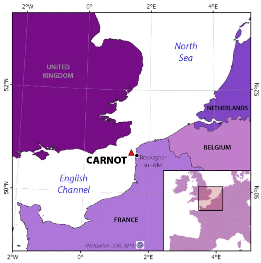
Carnot device used here is located in the eastern English Channel on the French coastal area. More 133
specifically, this automatic system is situated at the exit of the Boulogne-sur-Mer harbor on the Carnot 134
sea wall (50.7404 N; 1.5676 W) (Fig. 1). The Boulogne-sur-Mer harbor is the first fishing port in 135
France. Consequently, it is subjected to significant anthropogenic pollution. Moreover, the English 136
Channel has been affected by HAB generated by Phaeocystis for several decades (Lancelot et al. 137
1987; Lubac et al. 2008; Monchy et al. 2012; Danhiez et al. 2017). In the eastern part, this kind of 138
bloom has been a recurrent event since the 1990s (Spilmont et al. 2009; Schmitt et al. 2011; Houliez et 139
al. 2012; Grattepanche et al. 2011). This is one of the reasons for basing this kind of automated device 140
in this area. It is pivotal to consider that the English Channel has very turbid waters and is subject to 141
large tidal ranges. This has been tied to the fact that the bed of this sea is a continental shelf, with a 142
maximal depth of 180 meters. 143
8/44 144
145
Fig. 1. Location of the MAREL Carnot automatic device, in the eastern English Channel at the 146
Boulogne-sur-Mer port exit. 147
9/44
2.1.1. MAREL Carnot data
148
The MAREL Carnot sensors are attached to a floating system that nestles in a tube fixed to the 149
sea wall. The data are constantly recorded at a depth of 1.5 meters below sea level. However, the 150
measurement of the photosynthetically active radiation (P.A.R) parameter is an exception and for 151
obvious reasons, the sensor is not installed in the tube, but on the top of the sea wall. Each parameter 152
is recorded at a frequency of 20 minutes, except for the three nutrient parameters (nitrates, silicates, 153
and phosphates) which are recorded with a periodicity of 12 hours (Dur et al. 2007; Derot et al. 2015; 154
Zongo and Schmitt 2011; Huang and Schmitt 2014). Table 1 lists all the parameters that were used in 155
our study. The data presented here can be obtained from the following sites:
https://data.coriolis-156
cotier.org and the Seanoe site provided by Lefebvre et al. (2015). 157
Not all the available parameters, recorded by the MAREL device, have been used to avoid the 158
problems linked with collinearity. The term collinearity is used when the two predictors that are input 159
into a machine learning model, display a strong correlation. In order to decrease the computation time 160
and avoid creating an unstable model with a degraded predictive performance, it is better to avoid 161
selecting predictors showing correlations (Kuhn and Johnson 2013). To this end, we discarded the 162
readings for percentage of dissolved oxygen and salinity: they were too close to the concentration of 163
dissolved oxygen and the conductivity readings, respectively. In each case, we selected the parameter 164
with the most complete data set. 165
10/44
Time periods with missing data are an inherent problem for automatically generated datasets; 166
many factors can create these missing values: maintenance periods, internal system failures, and 167
vandalism (Dur et al. 2007; Derot et al. 2015). The percentage of missing data for each parameter is 168
listed in Table 1. The MAREL Carnot platform did not work for most of 2014. During the last four 169
years, the system experienced many problems; therefore, there is a high number of missing values for 170
many parameters. In order to avoid bias, our analysis only uses data between 2005 and 2010. In other 171
words, considering this 6-year period allows us to maintain consistency of the monitoring data used as 172
input to the RF model. In Fig. 2, we can see the averaged raw data for fluorescence and water 173
temperature for this time period of 6 years. Moreover, the type of machine learning used in this study 174
is able to manage the missing values (see Section 2.2.1 for further details). These missing values are 175
different for all the parameters. In some rare cases, some of these parameters could have more than 176
one month in raw missing values. In this context, we preferred to keep these missing values in the 177
inputs of the RF model, rather than using a numerical method to fill these gaps, which could create 178
greater bias. 179
11/44
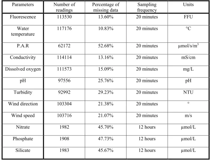
Table 1. Physicochemical parameters (target signal and predictors) in the original MAREL Carnot 180
database, with number of readings, percentage of missing data between 2005 and 2010, sampling 181
frequency, and their associated units. 182 Parameters Number of readings Percentage of missing data Sampling frequency Units
Fluorescence 113530 13.60% 20 minutes FFU
Water temperature
117176 10.83% 20 minutes °C
P.A.R 62172 52.68% 20 minutes µmol/s/m3
Conductivity 114114 13.16% 20 minutes mS/cm
Dissolved oxygen 111573 15.09% 20 minutes mg/L
pH 97556 25.76% 20 minutes pH
Turbidity 92992 29.23% 20 minutes NTU
Wind direction 103304 21.38% 20 minutes °
Wind speed 103716 21.07% 20 minutes m/s
Nitrate 1982 45.70% 12 hours µmol/L
Phosphate 1908 47.73% 12 hours µmol/L
Silicate 1983 45.67% 12 hours µmol/L
12/44 184
Fig. 2. Inter-annual mean (day-scale) of MAREL Carnot raw data for fluorescence and temperature 185
between 2005 and 2010. 186
13/44
2.2. Numerical analysis
187
2.2.1. Machine learning
188
There are many different types of machine learning models. The RF model is an evolution of 189
the classification and regression tree (CART) model, which was created by the same scientist in 1984 190
(Breiman et al. 1984). Contrary to the CART model that only uses one tree structure; the RF mode is 191
composed of a predetermined number of trees, hence the term “forest”. The input data of each tree 192
comes from a random sub-sampling performed with a bootstrap technique, hence the term “random”. 193
The first node of the tree is called the root node and split into two child nodes, and so forth until the 194
terminal nodes, which contain the prediction of the model. By following this step, the RF model in 195
regression mode will obtain an average between all the created trees. This stage is more generally 196
referred to as “ensemble learning”. For the RF model, this ensemble method is based on a cross 197
validation process via the out-of-bag (OOB) error. These OOB are mainly calculated from the mean 198
squared error (MSE) in the form of a ratio, in order to give a weight to each predictor. It is important 199
to note that these scores are ratio; therefore, they do not have units. The extraction of the OOB after 200
the learning phase allows us to examine the relative importance of each predictor. 201
Recent studies have shown that the RF model is well adapted to forecasting changes in the 202
phytoplankton community (Yajima and Derot 2018; Derot et al. 2020; Thomas et al. 2018). The tree 203
structure combined with the bootstrap allows the RF model to effectively manage missing values in 204
datasets, adapt to the study of nonlinear processes, and make no prior assumptions (Thomas et al. 205
2018; Breiman 2001). These properties coincide with the issues related to our long-term high-206
frequency sample database; the fluctuations in the phytoplankton abundance can be considered as a 207
stochastic process (Derot et al. 2015), leading to the many gaps associated with sampling automation 208
(see paragraph below). Within the framework of our study, the target signal is the phytoplankton 209
biomass, measured by a proxy via fluorescence. The predictors are the remaining physicochemical 210
parameters, as presented in Table 1. All our data are continuous; therefore, we used the RF model in 211
regression mode. 212
14/44
Moreover, we used an individual conditional expectation (ICE) plot (Goldstein et al. 2015), to 213
identify if the interactions created during the learning phase are comparable with the real biological 214
mechanisms. These ICE plots are an improvement on the partial dependence plot (PDP) used several 215
times in previous scientific studies on phytoplankton and water environments (Friedman et al. 2001; 216
Cutler et al. 2007; Roubeix et al. 2016; Teichert et al. 2016; Derot et al. 2020). The PDP highlights the 217
marginal effect between a selected predictor and the target signal (Friedman 2001). In this way, it is 218
possible to observe the global relationship between these two variables. The ICE plots allow a much 219
more refined vision, accounting for the individual effect of the observations on the target. To 220
summarize, the PDP corresponds to the average of the ICE; however this average curve may 221
overshadow the complexity of the relationship created by the model during the learning phase 222
(Goldstein et al. 2015). 223
All our numerical analyses were conducted using the MATLAB software and its “statistics 224
and machine learning” toolbox. We used the “TreeBagger” function for the RF models and
225
“plotPartialDependence” for the ICE plots. Once the learning is completed, the function 226
“TreeBagger” creates a “fitted model object”, which contains the model and all the related 227
information. By directly inserting this “object” in the function “oobError”, it is possible to observe the 228
evolution of the out-of-bag error (Figs A1-A4). The figures showing the ranking of predictor 229
importance (Figs 5, A6 and A9-A11) are also from the same “object”. We can extract these 230
permutation out-of-bag observations across each input, using the array 231
“OOBPermutedVarDeltaError”. We used the function “barh” to visualize these ranking. In addition, 232
the “rng” function was set to 1, in order to ensure that the results of the random draw could be used for 233
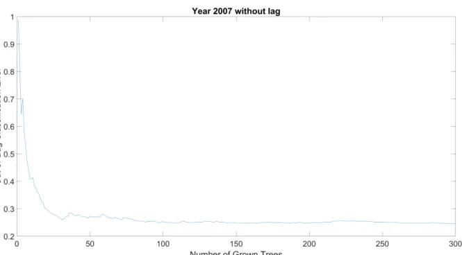
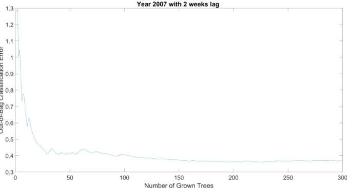
reproducibility purposes. In our preliminary studies, we observed that 300 trees were sufficient to 234
ensure the stability of the learning phases (Figs. A1 to A4). Given this, we performed all the RF runs 235
in this study using this number of trees. The minimal number of observations per node was set to 5 236
(Derot et al. 2020). 237
15/44
2.2.2. Forecast methodology
238
In order to understand the impact of the sampling frequency on the forecasts, we artificially 239
created three databases with the following time steps: 1 hour, 12 hours, and 1 day from the original 240
MAREL Carnot 20-minutes sample frequency database by performing a classical linear interpolation. 241
These interpolations were conducted using the MATLAB function “interp1” on all parameters; the 242
results are presented in Table 1. Subsequently, each of these datasets was split according to the year, 243
from 2005 to 2010, inclusively. As mentioned above, the coupling between machine learning and 244
hydrodynamic models could be a way to achieve decision-making tools (Jia et al. 2018; Hanson et al. 245
2020; Cuttitta et al. 2018). However, the calibration of the biogeochemistry solver linked to 246
hydrodynamic models is fairly sensitive and directly impacts on the capacity to reproduce the 247
dynamics of the phytoplankton (Shimoda and Arhonditsis 2016; Anderson 2005; Zhao et al. 2008). 248
This is why the parameterization of this kind of solver is generally performed year by year (Yajima 249
and Choi 2013). The division into annual subsets of our database was performed to meet this temporal 250
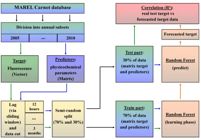
limitation. In all cases fluorescence is always the target signal (green boxes in Fig. 3) and the other 251
physicochemical parameters (Table 1) are the predictors (blue boxes in Fig. 3). 252
16/44
As in our previous phytoplankton forecast study (Yajima and Derot 2018), we used the sliding 253
window strategy to perform these forecasts (Herrera et al. 2010). To summarize, the sliding window is 254
a classical methodology for re-farming time series data when we a forecast analysis is to be performed 255
with machine learning models. A lag time is introduced between the target signal and the predictors. 256
For example, when the fluorescence is forecast with a lag time of one week, we removed the first 257
week of this target signal and the last week for all other physicochemical parameters (predictors). In 258
this way, a new input matrix is obtained, where the first value of the fluorescence corresponds to the 259
first value of day 8. The first values of all predictors are still the same. Therefore, there is always a 260
one-week lag between the target signal and the predictors. We used the following lag times for each of 261
our four databases and each year: no lag, 1 day, 3 days, 1 week, 2 weeks, 1 month, 2 months, 2 and a 262
half months and 3 months. Consequently, we performed nine RF runs for the1-year dataset. Therefore, 263
we made 45 RF runs for all the years in one database. In total, we performed 180 RF runs in this study 264
with our four datasets. It should be noted that by applying a sliding window of 2 weeks, we are forced 265
to remove some data at the beginning of the target signal vector and some data at the end of the 266
predictors’ matrix (Yajima and Derot 2018). In order to perform our analyses using the same amounts 267
of data, we cut the same time period for each case, depending on the largest lag time, that is. 3 months 268
(yellow boxes in Fig. 3). We applied the same procedure for these 180 cases (Fig. 3). 269
First, the fluorescence vector was identified as the target signal (green boxes and arrows in 270
Fig. 3), and the predictor matrix contained the other physicochemical parameters (blue boxes and 271
arrows in Fig. 3). Second, we applied the sliding window with one definite lag time, and cut periods 272
depending on the 3 months lag (yellow boxes in Fig. 3). Third, we split our data into two parts, the 273
training part comprised 70% of the cut and lagged data and the remaining percentage was used for the 274
test part (yellow boxes in Fig. 3). This split was realized with a semi-random draw via the MATLAB 275
function “cvpartition”. This function allowed the creation of two groups with similar intensity values. 276
17/44
Therefore, situations where in the training part contained all the high fluorescence values 277
(bloom periods), leaving the test part with no bloom values, or vice versa were accounted for and 278
skews in data were avoided. Fourth, we used the training part (both target and predictors) for the 279
learning phase of the RF model (orange boxes in Fig. 3). Fifth, we used only the predictors from the 280
test part to form a prediction or forecast of our target signal via the MATLAB function “predict”. 281
Finally, to control the quality of the predictions and forecasts; we performed a correlation between the 282
predicted target signal and the real data from the test part (red box in Fig. 3). These R² coefficients 283
were calculated with the coefficient of determination for each of our 180 cases as follows 284
(Shamshirband et al. 2019; Lee et al. 2016; Lee and Lee 2018; Recknagel et al. 2013; Du et al. 2018; 285 Kehoe et al. 2015): 286 287 𝑅!= 1 −𝑆𝑆"#$ 𝑆𝑆%&%= 1 − ∑( (𝑦'− 𝑦)')² ')* ∑( (𝑦'− 𝑦,) ')* ² 288 289
where 𝑆𝑆"#$ is the residual sum of squares, 𝑆𝑆%&% is the total sum of squares, 𝑛 is the number of 290
observations, 𝑦' is the observed data, 𝑦)' is the predicted data and 𝑦, is the mean of the observed data. 291
18/44 292
Fig. 3. Conceptual diagram presenting the methodology used to measure the forecast quality, 293
considering all lag times and sampling frequencies. 294
19/44
3. Results and discussion
295
The primary purpose of this study is to demonstrate the capacity of a machine learning model 296
to forecast phytoplankton blooms in coastal areas and to study the impact of the sampling frequency 297
on the forecast performance of the RF model. For that purpose, we artificially reduced the time step 298
and used different lag times with a sliding window strategy. First, we studied the evolution of the 299
coefficients of determination, depending on several lag times and sampling frequencies. Second, we 300
analyzed which predictors had the greatest influence on the learning phase. Subsequently, we 301
compared the interactions created by the RF model with real biological mechanisms. 302
303
3.1. Sampling frequency and time-lag impacts
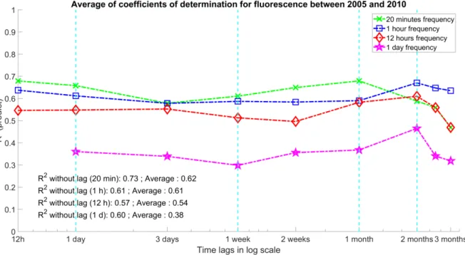
304The evolution of the forecast performances and the dependence on lag times is depicted in Fig. 305
4 for the four datasets up to a time period of 3 months. This analysis was only performed on the test 306
part. Each point on the four lines of Fig. 4 is derived from an inter-annual average for the years 2005-307
2010. For example, the second green point is calculated by averaging these 5 years with a lag time of 1 308
day. The time axis in Fig. 4 uses a log scale. Therefore, in order to avoid problems with the log of 309
zero, we have put the results for no lag time in the annotations for this figure. The calculated averages 310
of all lag times were included for each sampling frequency. Another point of view with the median 311
instead of average is presented in Fig. A7 in the appendix and the range of error in shown Table A1. 312
The green line in Fig. 4 represents the inter-annual average lag times depending on the sampling 313
frequency of 20 minutes. Similarly, the blue, red, and magenta lines represent the coefficient of 314
determination averages for the frequencies of 1 hour, 12 hours, and 1 day, respectively. It should be 315
noted that we cannot apply a sliding window of 12 hours for a sampling frequency of 1 day. This is 316
why the first point of the purple curve is missing in the Fig. 4. In the same way, the first point on the 317
red curve, which corresponds to the 12 hours frequency, is equal to its coefficient without lag; it has 318
been retained to maintain a visual coherence. 319
20/44
An example quantile-quantile plot from the test part is presented in the appendix (Fig. A5). 320
The highest coefficients of determination were obtained for the 20 minutes and 1 hour frequencies. 321
The accuracy of the RF model was evaluated for each frequency and lag time in the appendix in Fig. 322
A8. Table A2 shows the error range linked to this Fig. A8. The average coefficient is slightly better for 323
the green curve and R² with no lag time (see annotations). With respect to the frequencies of 12 hours 324
and 1 day, they have the smallest averages. It is significant to note that all curves exhibit the same 325
tendencies; R² generally starts to decrease after at two-month lag. 326
327
328
Fig. 4. Evolution of forecast performances depending on lag times and sampling frequencies from test 329
part. The y-axis represents the inter-annual average coefficient of determination from the outputs of 330
the RF models. The x-axis depicts the lag times from the sliding window on a logarithmic scale. The 331
green, blue, red and magenta lines correspond to the sampling frequencies of 20 minutes, 1 hour, 12 332
hours, and 1 day, respectively. The annotations show the coefficient of determination with no lag time 333
and the global averages of the coefficient of determination for each frequency. See Table A1 in the 334
appendix for the range of error. 335
21/44
Our results indicate that the RF model has the ability to use the supplementary information, 336
which is contained in the database from high-frequency sampling. As depicted in Fig. 4, the forecast 337
capacities are generally better for sampling frequencies of 20 minutes and 1 hour than those of 12 338
hours and 1 day. It is also evident that the average R² coefficient is less than 0.4 for a sampling 339
frequency of 1 day. In our previous works, we tested a close forecast strategy using another database 340
from fresh water ecosystems (Yajima and Derot 2018). It was a long-term dataset over a period of 30 341
years with a bimonthly sampling frequency. With this lower time step, in various cases the coefficients 342
of determination of the forecasted chlorophyll a were below a threshold of 0.5. In the current study 343
with high-frequency database, it is observed that R² stays above this threshold until the 2 months lag, 344
even when the sampling frequency is arterially decreased until 12 hours. Therefore, our findings 345
demonstrate that the pairing of an RF model with a high-frequency dataset from an automatic system 346
yields good forecast results on an annual scale. Water currents and phytoplankton migration have 347
greater significance in open-ocean and coastal areas than in lakes. This complexity could make it 348
difficult to obtain good forecast results for these types of ecosystems (Thomas et al. 2018). 349
22/44
Nevertheless, our study shows that this pairing strategy can also work in marine ecosystems. 350
Consequently, in a water body where water quality management is a major societal issue, it is of 351
pivotal importance to highlight the additional value provided by high sample frequency databases 352
generated by automatic devices. The results of this study indicate that the forecast performance of the 353
RF model increases with increasing sampling frequencies. In addition, it should be noted that although 354
some other studies in similar fields have used the pseudo-R² to measure the performance of the RF 355
model, the authors are aware that the coefficient does not assess the true forecast (Large et al. 2015; 356
Teichert et al. 2016; Thomas et al. 2018). Thus, we split our dataset between a learning part and a test 357
part (Fig. 3), and used the Pearson coefficient to measure the forecast performances. Consequently, the 358
pairing between machine learning models and automatically generated high sample frequency 359
databases could eventually lead to the creation of numerical decision-making models. Such a model 360
could help stakeholders prevent HABs from hindering the economy as well as human health. In the 361
next part of this section, we examine the influence of the predictors on the learning phase. 362
23/44
3.2. Physicochemical ranking
363
Once the learning phase has been completed, it is possible to extract the ranking predictor 364
importance from the out-of-bag (OOB) permutated error. Thus, we can understand the relative impact 365
that each predictor has on an RF model during the learning phase. As shown above, the original 366
MAREL Carnot database with a frequency of 20 minutes provided the best forecast results. In order to 367
examine the global ranking predictor importance, we performed an average of the 35 OOB errors for 368
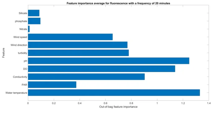
this frequency. The evaluated global ranking is presented in Fig. 5. It is observed that the nutrients 369
appear to have had low impacts. However, it must be noted that owing to the device limitations, with 370
the original time step of 20 minutes, these nutrients were actually recorded with a sampling frequency 371
of 12 hours (Table 1). In regard to the other physicochemical parameters, water temperature had the 372
most influence on these 35 learning phases, closely followed by the pH, and then the dissolved 373
oxygen. Furthermore, the fourth most important predictor is the salinity measured via its proxy for 374
conductivity. Apart from the nutrients, the photosynthetically active radiation (P.A.R) is the predictor 375
with the least influence. In the appendix, this global ranking has also been evaluated for the other 376
sampling frequencies: Fig. A9 for 1 hour, Fig. A10 for 12 hours and Fig. A11 for 1 day. 377
24/44 378
Fig. 5. Ranking of predictor importance based on the average of the out-of-bag (OOB) error, from the 379
35 runs performed with a time step of 20 minutes. Legend of abbreviations: P.A.R for 380
photosynthetically active radiation and DO for dissolved oxygen. 381
25/44
Water temperature, salinity, nutrients, dissolved oxygen, and pH are the water quality 382
indicators that are used in the water framework directive because of their direct impact on biological 383
processes (Best et al. 2007; Millero 2016). Among the physicochemical parameters, we temperature 384
and pH were observed to be the most important predictors, but the impact of the other predictors, such 385
as dissolved oxygen, turbidity, and salinity, are non-negligible. Furthermore, the sampling frequency 386
and lag time can also strongly impact the predictor ranking, as depicted in Fig. A6, where the out-of-387
bag importance of the temperature is very low. Despite its relative importance for a frequency of 20 388
minutes, the temperature alone is not sufficient to predict the chlorophyll a correctly. For this 389
frequency, we obtained an R² without lag that was equal to 0.31, when only the temperature was used 390
as a predictor and other physicochemical parameters were remove. The values of OOB that were 391
extracted from the 35 learning phases with at frequency of 20 minutes were consistent with the water 392
quality indicators, except for the nutrients (Fig 5). Nevertheless, if only the OOB from the databases 393
with a frequency over 12 hours were considered (Fig. A6); the nutrients crucially impacted the 394
learning phase of the RF models. This leads us to believe that the low impact of nutrients shown in this 395
high-frequency database is an artifact caused by recording system limitations. 396
Consequently, in light of the significant influence of the temperature on the learning phases of 397
the RF models, it considered to have been systematically account for when a parameter directly linked 398
to the primary production is predicted with machine learning based on tree structure. Furthermore, it is 399
important to harmonize all sampling frequencies from automatic devices in order to prevent this type 400
of bias. In this context, when designing or upgrading an automatic station, similar to a MAREL buoy, 401
having several types of sensors, we suggest installing sensors having the highest possible common 402
sampling frequency. This could increase the biological prediction linked to the phytoplankton biomass 403
via a machine learning model. Next, we will study the parallels between the interactions created by the 404
RF model and real biological mechanisms. 405
26/44
3.3. Learning phase interactions
406
Machine learning models are often considered “black boxes” because we cannot understand 407
the interaction between the predictor that the model creates during its learning phase. However, it is 408
possible to transform the RF models into “gray boxes” with the partial dependence plot (PDP) and the 409
individual conditional expectation (ICE) plots. In the previous section, it was seen that the water 410
temperature, conductivity, dissolved oxygen, and pH had the most influence on the average in our 411
learning phases. Therefore, we extracted one ICE plot for each of these 4 predictors with a time step of 412
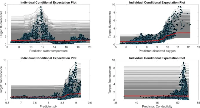
20 minutes (Fig.6). The red lines are the PDP, and all the gray lines and the blue points have been 413
derived from the ICE method. In reference to the water temperature, we can see that the RF model 414
predicts high fluorescence values mainly around 11.8°C; there is also a slight increment over 17.0°C. 415
The other three predictors exhibit a common pattern. That is to say, the predicted values of 416
fluorescence are low until the predictors reach a certain threshold. The results of this study exhibit 417
high predicted fluorescence values for a pH over 8.25, conductivity over 47 mS/cm, and concentration 418
in dissolved oxygen over 9 mg/L. It is also important to note that high fluorescence values are mainly 419
predicted for very high conductivities and pH values. However there is a large spread in the high 420
fluorescence values for the dissolved oxygen from the middle range to the higher value. 421
27/44 422
423
Fig. 6. Individual conditional expectation (ICE) plots for the four most influent predictors with a time 424
step of 20 minutes. The red lines denote the partial dependence plot (PDP); the gray lines and the blue 425
represent from the ICE analyses. Upper left: water temperature; upper right: dissolved oxygen; lower 426
left: pH; lower right: conductivity. 427
428 429
Although the interactions created during the learning phase of an RF model are difficult to 430
comprehend, it may be possible to obtain some links between these interactions and the biological 431
processes that occur in the ecosystems being studied. In Fig. 6 (upper left), It can be observed that the 432
highest fluorescence data are predicted for temperatures of approximately 11.8°C. This result is 433
consistent with those in previous literature (Schoemann et al. 2005; Jahnke 1989). The MAREL 434
Carnot device is located in the English Channel; in this area, the main issue is the harmful algal bloom 435
(HAB) linked to Phaeocystis globosa. For this type of phytoplankton, regardless of whether the light 436
conditions are limited, the optimal growth rate appears to be between 10°C and 14°C (Jahnke 1989; 437
Schoemann et al. 2005). Therefore, our ICE analysis of water temperature illustrates that even without 438
prior assumptions, an RF model can account for some real biological processes. 439
28/44
4. Conclusion
440
In this study we found that the average coefficient of determination, which is the index of the 441
quality of the forecast, decreases when the sampling frequency increases. The coefficient for the 20-442
minute time step was 0.24 larger than that for the 1-day time step. From our analyses, we observed 443
that the nutrients had a limited impact on the learning phase with the highest sampling frequency. In 444
regard to the water temperature, the averaged OOB error reached 13, while that for the phosphate 445
concentration was only approximately 0.1. Creation of the ICE plot for the water temperature allowed 446
us to illustrate that the RF model predicted the highest fluorescence values of approximately 11.8°C. 447
Consequently, the results suggest that RF models can use the additional information contained in high-448
frequency databases. It is supposed that the apparent low influence of the nutrients was a bias due to 449
the difference in sampling frequencies. Moreover, although the RF model has no prior assumptions, it 450
was able to create some interactions closely resembling the biological processes present in our study 451
area. 452
The decrease in the sampling frequency is not the only factor impacting forecast capacity. It 453
should be kept in mind that different time steps between the input parameters can introduce biases into 454
the learning process of an RF model. Therefore, it is imperative to have harmonized sampling 455
frequencies in datasets from automated devices. Several studies in the environmental science literature 456
have claimed that the pairing between high-frequency or long-term datasets with an RF model could 457
overcome the limitations of conventional models (linear, generalized linear model …) (Kehoe et al. 458
2015; Thomas et al. 2018; Rivero-Calle et al. 2015). The results of our study seem to confirm this 459
hypothesis. 460
29/44
Furthermore, some of the automatic systems are equipped with flow cytometers, enabling 461
differentiation between the phytoplankton groups responsible for the HAB (Thomas et al. 2018). 462
Therefore, pairing these types of datasets with machine learning models could aid in the creation of 463
numerical decision-making tools that can help stakeholders with water quality management. In the 464
long run, this kind of tool could have a benefit the economy and human health. Within this framework, 465
we are currently exploring the possibilities of applying this type of pairing on an inter-annual scale, in 466
order to increase the lengths of the forecasted periods. 467
30/44 Acknowledgements
468
This research was funded by a grant from the Japan Society for the Promotion of Science (JSPS). 469
Derot J. benefited of Postdoctoral Fellowship for Research in Japan. The MAREL Carnot system 470
belongs to a fixed platform network along French coasts called COAST-HF (http://coast-hf.fr). The 471
data presented here can be obtained in the following sites: https://data.coriolis-cotier.org and also the 472
Seanoe site given in Lefebvre et al. (2015). 473
31/44
References
474
Anderson, T. R. (2005). Plankton functional type modelling: running before we can walk? Journal of 475
Plankton Research, 27(11), 1073-1081. http://dx.doi.org/10.1093/plankt/fbi076
476 477
Anderson, D. M., Glibert, P. M., & Burkholder, J. M. (2002). Harmful algal blooms and 478
eutrophication: nutrient sources, composition, and consequences. Estuaries, 25(4), 704-726. 479
http://dx.doi.org/10.1007/BF02804901
480 481
Backer, L., Manassaram-Baptiste, D., LePrell, R., & Bolton, B. (2015). Cyanobacteria and algae 482
blooms: review of health and environmental data from the harmful algal bloom-related illness 483
surveillance system (HABISS) 2007–2011. Toxins, 7(4), 1048-1064. 484
http://dx.doi.org/10.3390/toxins7041048
485 486
Bae, S., & Seo, D. (2018). Analysis and modeling of algal blooms in the Nakdong River, Korea. 487
Ecological modelling, 372, 53-63. http://dx.doi.org/10.1016/j.ecolmodel.2018.01.019
488 489
Best, M., Wither, A., & Coates, S. (2007). Dissolved oxygen as a physico-chemical supporting 490
element in the Water Framework Directive. Marine pollution bulletin, 55(1-6), 53-64. 491
http://dx.doi.org/10.1016/j.marpolbul.2006.08.037
492 493
Breiman, L. (2001). Random forests. Machine learning, 45(1), 5-32. 494
495
Breiman, L., Friedman, J., Olshen, R., & Stone, C. (1984). Classification and regression trees. 496
Wadsworth Int. Group, 37(15), 237-251. http://dx.doi.org/10.1201/9781315139470
497 498
Burkholder, J. M. (2003). Cyanobacteria. Encyclopedia of Environmental Microbiology. 499
500
Camargo, J. A., & Alonso, Á. (2006). Ecological and toxicological effects of inorganic nitrogen 501
pollution in aquatic ecosystems: a global assessment. Environment international, 32(6), 831-502
849. http://dx.doi.org/10.1016/j.envint.2006.05.002
503 504
Carmichael, W. W., & Boyer, G. L. (2016). Health impacts from cyanobacteria harmful algae blooms: 505
Implications for the North American Great Lakes. Harmful algae, 54, 194-212. 506
http://dx.doi.org/10.1016/j.hal.2016.02.002
507 508
Chen, Q., Guan, T., Yun, L., Li, R., & Recknagel, F. (2015). Online forecasting chlorophyll a 509
concentrations by an auto-regressive integrated moving average model: Feasibilities and 510
potentials. Harmful algae, 43, 58-65. http://dx.doi.org/10.1016/j.hal.2015.01.002
511 512
Chen, Y.-Q., Wang, N., Zhang, P., Zhou, H., & Qu, L.-H. (2002). Molecular evidence identifies 513
bloom-forming Phaeocystis (Prymnesiophyta) from coastal waters of southeast China as 514
Phaeocystis globosa. Biochemical Systematics and Ecology, 30(1), 15-22. 515
http://dx.doi.org/10.1016/S0305-1978(01)00054-0
516 517
Cho, H., Choi, U., & Park, H. (2018). Deep learning application to time-series prediction of daily 518
chlorophyll-a concentration. WIT Trans. Ecol. Environ, 215, 157-163. 519
http://dx.doi.org/10.2495/EID180141
520 521
Cho, H., & Park, H. Merged-LSTM and multistep prediction of daily chlorophyll-a concentration for 522
algal bloom forecast. In IOP Conference Series: Earth and Environmental Science, 2019 (Vol. 523
351, pp. 012020, Vol. 1): IOP Publishing http://dx.doi.org/10.1088/1755-1315/351/1/012020
32/44
Cutler, D. R., Edwards Jr, T. C., Beard, K. H., Cutler, A., Hess, K. T., Gibson, J., et al. (2007). 525
Random forests for classification in ecology. Ecology, 88(11), 2783-2792. 526
http://dx.doi.org/10.1890/07-0539.1
527 528
Cuttitta, A., Torri, M., Zarrad, R., Zgozi, S., Jarboui, O., Quinci, E. M., et al. (2018). Linking surface 529
hydrodynamics to planktonic ecosystem: the case study of the ichthyoplanktonic assemblages 530
in the Central Mediterranean Sea. Hydrobiologia, 821(1), 191-214. 531
http://dx.doi.org/10.1007/s10750-017-3483-x
532 533
Danhiez, F., Vantrepotte, V., Cauvin, A., Lebourg, E., & Loisel, H. (2017). Optical properties of 534
chromophoric dissolved organic matter during a phytoplankton bloom. Implication for DOC 535
estimates from CDOM absorption. Limnology and Oceanography, 62(4), 1409-1425. 536
http://dx.doi.org/10.1002/lno.10507
537 538
Derot, J., Jamoneau, A., Teichert, N., Rosebery, J., Morin, S., & Laplace-Treyture, C. (2020). 539
Response of phytoplankton traits to environmental variables in French lakes: New 540
perspectives for bioindication. Ecological indicators, 108, 105659. 541
http://dx.doi.org/10.1016/j.ecolind.2019.105659
542 543
Derot, J., Schmitt, F. G., Gentilhomme, V., & Morin, P. (2016). Correlation between long-term marine 544
temperature time series from the eastern and western English Channel: Scaling analysis using 545
empirical mode decomposition. Comptes Rendus Géoscience, 348(5), 343-349. 546
http://dx.doi.org/10.1016/j.crte.2015.12.001
547 548
Derot, J., Schmitt, F. G., Gentilhomme, V., & Zongo, S. B. (2015). Long-term high frequency 549
phytoplankton dynamics, recorded from a coastal water autonomous measurement system in 550
the eastern English Channel. Continental Shelf Research, 109, 210-221. 551
http://dx.doi.org/10.1016/j.csr.2015.09.015
552 553
Du, Z., Qin, M., Zhang, F., & Liu, R. (2018). Multistep-ahead forecasting of chlorophyll a using a 554
wavelet nonlinear autoregressive network. Knowledge-Based Systems, 160, 61-70. 555
http://dx.doi.org/10.1016/j.knosys.2018.06.015
556 557
Dur, G., Schmitt, F. G., & Souissi, S. (2007). Analysis of high frequency temperature time series in 558
the Seine estuary from the Marel autonomous monitoring buoy. Hydrobiologia, 588(1), 59-68. 559
http://dx.doi.org/10.1007/s10750-007-0652-3
560 561
Edwards, K. F., Thomas, M. K., Klausmeier, C. A., & Litchman, E. (2016). Phytoplankton growth and 562
the interaction of light and temperature: A synthesis at the species and community level. 563
Limnology and Oceanography, 61(4), 1232-1244. http://dx.doi.org/10.1002/lno.10282
564 565
Friedman, J. H. (2001). Greedy function approximation: a gradient boosting machine. Annals of 566
statistics, 1189-1232. 567
568
Friedman, J., Hastie, T., & Tibshirani, R. (2001). The elements of statistical learning (Vol. 1, Vol. 10): 569
Springer series in statistics New York, NY, USA:. 570
571
Glibert, P. M., Anderson, D. M., Gentien, P., Granéli, E., & Sellner, K. G. (2005). The global, 572
complex phenomena of harmful algal blooms. http://dx.doi.org/10.5670/oceanog.2005.49
573 574
Goldstein, A., Kapelner, A., Bleich, J., & Pitkin, E. (2015). Peeking inside the black box: Visualizing 575
statistical learning with plots of individual conditional expectation. Journal of Computational 576
and Graphical Statistics, 24(1), 44-65. http://dx.doi.org/10.1080/10618600.2014.907095
33/44
Grattepanche, J.-D., Breton, E., Brylinski, J.-M., Lecuyer, E., & Christaki, U. (2011). Succession of 578
primary producers and micrograzers in a coastal ecosystem dominated by Phaeocystis globosa 579
blooms. Journal of Plankton Research, 33(1), 37-50. http://dx.doi.org/10.1093/plankt/fbq097
580 581
Hanson, P. C., Stillman, A. B., Jia, X., Karpatne, A., Dugan, H. A., Carey, C. C., et al. (2020). 582
Predicting lake surface water phosphorus dynamics using process-guided machine learning. 583
Ecological modelling, 430, 109136. http://dx.doi.org/10.1016/j.ecolmodel.2020.109136
584 585
Heisler, J., Glibert, P. M., Burkholder, J. M., Anderson, D. M., Cochlan, W., Dennison, W. C., et al. 586
(2008). Eutrophication and harmful algal blooms: a scientific consensus. Harmful algae, 8(1), 587
3-13. http://dx.doi.org/10.1016/j.hal.2008.08.006
588 589
Houliez, E., Lizon, F., Thyssen, M., Artigas, L. F., & Schmitt, F. G. (2012). Spectral fluorometric 590
characterization of Haptophyte dynamics using the FluoroProbe: an application in the eastern 591
English Channel for monitoring Phaeocystis globosa. Journal of Plankton Research, 34(2), 592
136-151. http://dx.doi.org/10.1093/plankt/fbr091
593 594
Herrera, M., Torgo, L., Izquierdo, J., & Pérez-García, R. (2010). Predictive models for forecasting 595
hourly urban water demand. Journal of Hydrology, 387(1-2), 141-150. 596
http://dx.doi.org/10.1016/j.jhydrol.2010.04.005
597 598
Howarth, R. W., Anderson, D., Cloern, J. E., Elfring, C., Hopkinson, C. S., Lapointe, B., et al. (2000). 599
Nutrient pollution of coastal rivers, bays, and seas. Issues in ecology(7), 1-16. 600
601
Huang, Y., & Schmitt, F. G. (2014). Time dependent intrinsic correlation analysis of temperature and 602
dissolved oxygen time series using empirical mode decomposition. Journal of Marine 603
Systems, 130, 90-100. http://dx.doi.org/10.1016/j.jmarsys.2013.06.007
604 605
Jahnke, J. (1989). The light and temperature dependence of growth rate and elemental composition of 606
Phaeocystis globosa Scherffel and P. pouchetii (Har.) Lagerh. in batch cultures. Netherlands 607
Journal of Sea Research, 23(1), 15-21. http://dx.doi.org/10.1016/0077-7579(89)90038-0
608 609
Jia, X., Karpatne, A., Willard, J., Steinbach, M., Read, J., Hanson, P. C., et al. (2018). Physics guided 610
recurrent neural networks for modeling dynamical systems: Application to monitoring water 611
temperature and quality in lakes. arXiv preprint arXiv:1810.02880. 612
613
Kehoe, M. J., Chun, K. P., & Baulch, H. M. (2015). Who smells? Forecasting taste and odor in a 614
drinking water reservoir. Environmental science & technology, 49(18), 10984-10992. 615
http://dx.doi.org/10.1021/acs.est.5b00979
616 617
Kuhn, M., & Johnson, K. (2013). Applied predictive modeling (Vol. 26): Springer. 618
http://dx.doi.org/10.1007/978-1-4614-6849-3
619 620
Lancelot, C., Billen, G., Sournia, A., Weisse, T., Colijn, F., Veldhuis, M. J., et al. (1987). Phaeocystis 621
blooms and nutrient enrichment in the continental coastal zones of the North Sea. Ambio(1). 622
623
Lancelot, C., Rousseau, V., Schoemann, V., & Becquevort, S. (2002). On the ecological role of the 624
different life forms of Phaeocystis. LIFEHAB: Life history of microalgal species causing 625
harmful blooms. European Commission publication no: EUR, 20361, 71-75.
626 627
Lapointe, B. E., Herren, L. W., & Paule, A. L. (2017). Septic systems contribute to nutrient pollution 628
and harmful algal blooms in the St. Lucie Estuary, Southeast Florida, USA. Harmful algae, 70, 629
1-22. http://dx.doi.org/10.1016/j.hal.2017.09.005
34/44
Large, S. I., Fay, G., Friedland, K. D., & Link, J. S. (2015). Quantifying patterns of change in marine 631
ecosystem response to multiple pressures. PloS one, 10(3), e0119922. 632
http://dx.doi.org/10.1371/journal.pone.0119922
633 634
Lee, G., Bae, J., Lee, S., Jang, M., & Park, H. (2016). Monthly chlorophyll-a prediction using neuro-635
genetic algorithm for water quality management in Lakes. Desalination and Water Treatment, 636
57(55), 26783-26791. http://dx.doi.org/10.1080/19443994.2016.1190107
637 638
Lee, S., & Lee, D. (2018). Improved prediction of harmful algal blooms in four Major South Korea’s 639
Rivers using deep learning models. International journal of environmental research and public 640
health, 15(7), 1322. http://dx.doi.org/10.3390/ijerph15071322
641 642
Lefebvre, A. (2015). MAREL Carnot data and metadata from Coriolis Data Centre. SEANOE. 643
644
Lubac, B., Loisel, H., Guiselin, N., Astoreca, R., Artigas, L. F., & Mériaux, X. (2008). Hyperspectral 645
and multispectral ocean color inversions to detect Phaeocystis globosa blooms in coastal 646
waters. Journal of Geophysical Research: Oceans, 113(C6). 647
http://dx.doi.org/10.1029/2007JC004451
648 649
Millero, F. J. (2016). Chemical oceanography: CRC press. http://dx.doi.org/10.1201/b14753
650 651
Monchy, S., Grattepanche, J.-D., Breton, E., Meloni, D., Sanciu, G., Chabé, M., et al. (2012). 652
Microplanktonic community structure in a coastal system relative to a Phaeocystis bloom 653
inferred from morphological and tag pyrosequencing methods. PloS one, 7(6), e39924. 654
http://dx.doi.org/10.1371/journal.pone.0039924
655 656
Pennekamp, F., Iles, A. C., Garland, J., Brennan, G., Brose, U., Gaedke, U., et al. (2019). The intrinsic 657
predictability of ecological time series and its potential to guide forecasting. Ecological 658
Monographs, e01359. http://dx.doi.org/10.1002/ecm.1359
659 660
Recknagel, F., Ostrovsky, I., Cao, H., Zohary, T., & Zhang, X. (2013). Ecological relationships, 661
thresholds and time-lags determining phytoplankton community dynamics of Lake Kinneret, 662
Israel elucidated by evolutionary computation and wavelets. Ecological modelling, 255, 70-663
86. http://dx.doi.org/10.1016/j.ecolmodel.2013.02.006
664 665
Reynaud, A., & Lanzanova, D. (2017). A global meta-analysis of the value of ecosystem services 666
provided by lakes. Ecological Economics, 137, 184-194. 667
http://dx.doi.org/10.1016/j.ecolecon.2017.03.001
668 669
Rivero-Calle, S., Gnanadesikan, A., Del Castillo, C. E., Balch, W. M., & Guikema, S. D. (2015). 670
Multidecadal increase in North Atlantic coccolithophores and the potential role of rising CO2. 671
Science, 350(6267), 1533-1537. http://dx.doi.org/10.1126/science.aaa8026
672 673
Roelke, D. L., Grover, J. P., Brooks, B. W., Glass, J., Buzan, D., Southard, G. M., et al. (2010). A 674
decade of fish-killing Prymnesium parvum blooms in Texas: roles of inflow and salinity. 675
Journal of plankton research, 33(2), 243-253. http://dx.doi.org/10.1093/plankt/fbq079
676 677
Roubeix, V., Danis, P.-A., Feret, T., & Baudoin, J.-M. (2016). Identification of ecological thresholds 678
from variations in phytoplankton communities among lakes: contribution to the definition of 679
environmental standards. Environmental monitoring and assessment, 188(4), 246. 680
http://dx.doi.org/10.1007/s10661-016-5238-y
35/44
Schindler, D. W. (2006). Recent advances in the understanding and management of eutrophication. 682
Limnology and Oceanography, 51(1part2), 356-363.
683
http://dx.doi.org/10.4319/lo.2006.51.1_part_2.0356
684 685
Schmitt, F. G., Landry, Y., Revillion, M., Bordé, C., Gentilhomme, V., & Herbert, V. (2011). Blooms 686
de Phaeocystis sur la Côte d'Opale: investigations historiques, in Du naturalisme à l'écologie, 687
edité par FG Schmitt. 688
689
Schmitt, F.G., & Lefebvre A. (2016). Mesures à haute résolution dans l’environnement marin côtie. 690
Paris: CNRS Editions. 691
692
Schoemann, V., Becquevort, S., Stefels, J., Rousseau, V., & Lancelot, C. (2005). Phaeocystis blooms 693
in the global ocean and their controlling mechanisms: a review. Journal of Sea Research, 694
53(1-2), 43-66. http://dx.doi.org/10.1016/j.seares.2004.01.008
695 696
Shimoda, Y., & Arhonditsis, G. B. (2016). Phytoplankton functional type modelling: running before 697
we can walk? A critical evaluation of the current state of knowledge. Ecological modelling, 698
320, 29-43. http://dx.doi.org/10.1016/j.ecolmodel.2015.08.029
699 700
Shamshirband, S., Jafari Nodoushan, E., Adolf, J. E., Abdul Manaf, A., Mosavi, A., & Chau, K.-w. 701
(2019). Ensemble models with uncertainty analysis for multi-day ahead forecasting of 702
chlorophyll a concentration in coastal waters. Engineering Applications of Computational 703
Fluid Mechanics, 13(1), 91-101. http://dx.doi.org/10.1016/j.ecolmodel.2015.08.029
704 705
Shin, J., Yoon, S., & Cha, Y. (2017). Prediction of cyanobacteria blooms in the lower Han River 706
(South Korea) using ensemble learning algorithms. Desalination and Water Treatment, 84, 31-707
39. http://dx.doi.org/10.5004/dwt.2017.20986
708 709
Smith, V. H., Joye, S. B., & Howarth, R. W. (2006). Eutrophication of freshwater and marine 710
ecosystems. Limnology and Oceanography, 51(1part2), 351-355. 711
http://dx.doi.org/10.4319/lo.2006.51.1_part_2.0351
712 713
Spilmont, N., Denis, L., Artigas, L. F., Caloin, F., Courcot, L., Créach, A., et al. (2009). Impact of the 714
Phaeocystis globosa spring bloom on the intertidal benthic compartment in the eastern English 715
Channel: A synthesis. Marine pollution bulletin, 58(1), 55-63. 716
http://dx.doi.org/10.1016/j.marpolbul.2008.09.007
717 718
Teichert, N., Borja, A., Chust, G., Uriarte, A., & Lepage, M. (2016). Restoring fish ecological quality 719
in estuaries: implication of interactive and cumulative effects among anthropogenic stressors. 720
Science of the Total Environment, 542, 383-393.
721
http://dx.doi.org/10.1016/j.scitotenv.2015.10.068
722 723
Thomas, M. K., Fontana, S., Reyes, M., Kehoe, M., & Pomati, F. (2018). The predictability of a lake 724
phytoplankton community, over time‐scales of hours to years. Ecology letters, 21(5), 619-628. 725
http://dx.doi.org/10.1111/ele.12927
726 727
Veldhuis, M. J., & Wassmann, P. (2005). Bloom dynamics and biological control of a high biomass 728
HAB species in European coastal waters: a Phaeocystis case study. Harmful algae, 4(5), 805-729
809. http://dx.doi.org/10.1016/j.hal.2004.12.004
730 731
Yajima, H., & Choi, J. (2013). Changes in phytoplankton biomass due to diversion of an inflow into 732
the Urayama Reservoir. Ecological engineering, 58, 180-191. 733
http://dx.doi.org/10.1016/j.ecoleng.2013.06.030
36/44
Yajima, H., & Derot, J. (2018). Application of the Random Forest model for chlorophyll-a forecasts in 735
fresh and brackish water bodies in Japan, using multivariate long-term databases. Journal of 736
Hydroinformatics, 20(1), 206-220. http://dx.doi.org/10.2166/hydro.2017.010
737 738
Zhang, F., Wang, Y., Cao, M., Sun, X., Du, Z., Liu, R., et al. (2016). Deep-learning-based approach 739
for prediction of algal blooms. Sustainability, 8(10), 1060. 740
http://dx.doi.org/10.3390/su8101060
741 742
Zhao, J., Ramin, M., Cheng, V., & Arhonditsis, G. B. (2008). Competition patterns among 743
phytoplankton functional groups: How useful are the complex mathematical models? acta 744
oecologica, 33(3), 324-344. http://dx.doi.org/10.1016/j.actao.2008.01.007
745 746
Zongo, S., & Schmitt, F. G. (2011). Scaling properties of pH fluctuations in coastal waters of the 747
English Channel: pH as a turbulent active scalar. Nonlinear Processes in Geophysics, 18(6), 748
829-839. http://dx.doi.org/10.5194/npg-18-829-2011 749
37/44
Appendix
750
751
Fig. A1. Evolution of the out-of-bag error for the year 2007 without lag time. 752
753 754
755
Fig. A2. Evolution of the out-of-bag error for the year 2007 with lag time of 1 day. 756
38/44 757
Fig. A3. Evolution of the out-of-bag error for the year 2007 with lag time of 2 weeks. 758
759 760
761
Fig. A4. Evolution of the out-of-bag error for the year 2007 with lag time of 2 months. 762
39/44 763
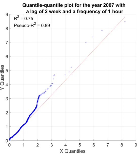
Fig. A5. Quantile-quantile plot from the test part; for the year 2007 with a frequency of 1 hour and a 764
lag time of 2 weeks. 765
40/44 767
Fig. A6. Ranking of predictor importance from the out-of-bag (OOB) error, for the year 2007 this a 768
lag time of 1 day and a sampling frequency of 1 day. 769 770 Frequency 20 minutes Frequency 1 hours Frequency 12 hours Frequency 1 day Lag = 0 0.14 0.23 0.13 0.07 Lag = 12 hours 0.05 0.15 0.19 ∅ Lag = 1 day 0.07 0.17 0.18 0.26 Lag = 3 days 0.13 0.16 0.18 0.26 Lag = 1 week 0.10 0.15 0.20 0.21 Lag = 2 weeks 0.09 0.20 0.21 0.23 Lag = 1 month 0.06 0.16 0.18 0.21 Lag = 2 months 0.12 0.09 0.11 0.21 Lag = 2.5 month 0.15 0.08 0.20 0.19 Lag = 3 months 0.15 0.09 0.30 0.23
Table A1. Error ranges linked to Fig. 4 calculated via the standard deviation. 771
41/44 772
Fig. A7. Evolution of forecast performances depending on lag times and sampling frequencies from 773
test part. The y-axis represents the inter-annual median from the outputs of the RF models. The x-axis 774
denotes the lag times from the sliding window on a logarithmic scale. The green, blue, red and 775
magenta lines correspond to the sampling frequencies of 20 minutes, 1 hour, 12 hours, and 1 day, 776
respectively. The annotations display the median of coefficient of determination with no lag time for 777
each frequency. 778