Table of Content
1.
DATA FOR THE LAB-SCALE PROCESSES ... 2
2.
DATA FOR THE (FUTURE) PILOT PRODUCTION ... 4
3.
(BACKGROUND) LIFE CYCLE INVENTORY DATASETS ... 9
3.1.
Benzyl ether ... 9
3.2.
Cobalt chloride ... 10
3.3.
Cobalt hydroxide ... 11
3.4.
Lithium alkoxides and aryloxides ... 12
3.5.
Oleylamine ... 17
3.6.
Manganese acetate ... 19
3.7.
Solvent recycling ... 20
4.
RESULTS OF LCA-CALCULATIONS ... 21
4.1.
Lab-Scale ... 21
4.2.
(future) Pilot Production ... 22
4.3.
Comparison with other cathode materials ... 23
1. DATA FOR THE LAB-SCALE PROCESSES
On the Lab-Scale, the foreground system is split into the following, three different production steps: [i] synthesis of Li-containing materials (LiCoO2 and LiMnPO4 respectively),
[ii] production of composite material, and finally
[iii] production of electrode, i.e. by applying the composite material on an aluminium foil in order to form the complete cathode.
Main data source for these foreground processes are the practical experiments executed by the authors at University of Fribourg concerning the synthesis of these various materials; and additional, mainly literature data in order to cover specific points/questions for all those situations, where the analysis of the experiments did not result in detailed enough information. From Table S.1 to Table S.3, the values from these practical experiments are summarized, together with their respective translation into an LCA language.
Table S.1 Input and output data for the production of LiCoO2 via the various, here examined pathways
Material Unit amount Remarks
meth eth iso t-but phen mix
(i) Inputs
Lithium alkoxide1 kg 1.300 3.938 2.434 2.882 4.713 3.225
Cobalt chloride kg 1.478 1.642 1.602 1.565 1.529 1.494
Tetrahydrofuran2 kg 14.326 15.918 15.534 24.270 23.712 23.179 Density 0.889 kg/L
Methanol2 kg 3.573 - - - Density 0.792 kg/L
Argon (gaseous) kg 5.563 6.181 6.033 5.891 5.755 5.626 Density 1.669 kg/m3
Nitrogen (liquid) kg 361 401 391 382 373 365 Density 0.812 kg/L Water, deionised kg 278 309 301 294 287 281
Electricity kWh 90.6 96.7 103 109.2 110.1 125.3 (ii) Outputs
Lithium cobalt oxide kg 1 Product
Lithium chloride kg 0.956 2.674 1.036 1.012 0.995 0.973 Co-product3
Solvent, to recycling kg 59.356 53.242 51.959 82.120 80.232 78.429
Waste for disposal kg 0.144 0.272 0.241 0.212 0.184 0.180
Carbon dioxide, to air kg 1.444 6.543 4.819 6.235 12.414 7.865
Tetrahydrofuran, to air kg 1.667 1.852 1.807 1.765 3.333 3.258
Methanol, to air kg 1.046 - - - - -
1
meth: lithium methoxide pathway (default assumption for modelling) / eth: lithium ethoxide pathway / iso: lithium isopro-poxide pathway / t-but: lithium tert-butoxide pathway / phen: lithium phenoxide pathway / mix: pathway with mixture of Li tert-butoxide and Li phenoxide
2
reported here is the amount, taking into account the recycled proportion of THF resp. methanol (i.e. the value represents each time those part that can’t be recycled, and thus is actually “consumed” in the production process)
3
For the default calculation on the lab-scale level, lithium chloride has been considered as by-product, i.e. all the impacts have been allocated to LiCoO2 (i.e. a conservative approach is chosen like this).
A sensitivity calculation, using a mass-based allocation of all inputs and outputs results for the default pathway (i.e. pathway using lithium methoxide as starting material) in a reduction of the impacts by a factor of 4; due to the high amount of LiCl produced simultaneously in the examined chemical process – and this independent from the impact
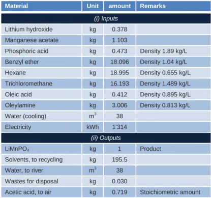
Table S.2 Input and output data for the production of LiMnPO4
Material Unit amount Remarks
(i) Inputs
Lithium hydroxide kg 0.378
Manganese acetate kg 1.103
Phosphoric acid kg 0.473 Density 1.89 kg/L
Benzyl ether kg 18.096 Density 1.04 kg/L
Hexane kg 18.995 Density 0.655 kg/L
Trichloromethane kg 16.193 Density 1.489 kg/L
Oleic acid kg 0.412 Density 0.895 kg/L
Oleylamine kg 3.006 Density 0.813 kg/L Water (cooling) m3 38 Electricity kWh 1’314 (ii) Outputs LiMnPO4 kg 1 Product Solvents, to recycling kg 195.5 Water, to river m3 38
Wastes for disposal kg 0.030
Acetic acid, to air kg 0.719 Stoichiometric amount
Table S.3 Input and output data for the production of the composite and the electrode materials, out of the Li-containing materials (LiCoO2 resp. LiMnPO4)
Material Unit composite
material electrode material Remarks (i) Inputs Li-containing material kg 0.833 Composite material kg 0.857 Carbon (SFG) kg 0.168 PVDF kg 0.071 NMP kg 0.736 Density 1.03 kg/L SP Carbon kg 0.071 Electricity kWh 63.3 7.665 (ii) Outputs
Composite material kg 1 Product
Electrode material kg 1 Product
Wastes for disposal kg 0.001 0.1
NMP, to air kg 0.736
Carbon (SFG): name for graphite provided by the producer PVDF: Polyvinylidenfluoride
NMP: N-Methyl-2-pyrrolidon
2. DATA FOR THE (FUTURE) PILOT PRODUCTION
Starting point for the up-scaled inventory data of the two different Li-containing materials are the above listed lab-scale data from the experiments at the University of Fribourg. In Table S.4 and Table S.5 on the next two pages, the resulting values for a (future) pilot production are reported, together with a short description how these numbers have been derived from the lab-scale data. For LiCoO2,
the pathway with lithium methoxide as starting material is used here – due to economic reasons (this pathway has the lowest costs) this seems to be the most promising option among the pathways for the LiCoO2 production examined on the Lab-scale.
Table S.4 Input and output data for the pilot production of LiCoO2 (via the methoxide pathway)
Material Unit Upscaling Derivation of / Assumptions for upscaled data High Low
(i) Inputs
Lithium methoxide kg 1.202 1.158 Assumed is a yield of 85% (high) and 90% (low) for Chloride consumption in overall process; and based on this a yield of 90% (high) and 95% (low) is assumed for lithium methoxide and 95% (high) and 98% (low) for CoCl2 (in accordance with the modelling of chemical production processes reported in Hischier et al., 2005)
Cobalt chloride kg 1.396 1.354
Tetrahydrofuran kg 0.025 0.012 Due to the “closed” system (as a batch process is assumed), the total THF amount is reduced to 20% (high) and 10% (low) compared to lab-scale process – and thereof, it is assumed that 2.5% are lost (and need to be replaced as an input); while the remaining 97.5% are recovered by an (internal) distillation process. Furthermore, it is assumed that THF is in large parts replaced by Methanol (MeOH) – i.e. we assume here that 90% of THF are replaced, and only 10% are still consumed in form of THF.
Methanol kg 0.284 0.142 In addition to the above-mentioned amount of 90% of the THF, the MeOH input from the lab-scale process is (due to assumed “closed” system with a batch process) reduced to 10% compared to the lab-scale process – and from this total again 2.5% are lost (and need to be replaced as an input); while the remaining 97.5% are recovered by an (internal) distillation process.
Argon kg - 100% replaced by gaseous nitrogen
Nitrogen (gaseous) kg 1.950 1.560 Assumption: use of 40% of Ar amount (in m3) in Lab-Scale process
Nitrogen (liquid) kg - Not needed anymore (i.e. 100% reduction)
Water, deionised kg 55.6 Assumption: 80% less than in the Lab-Scale process Electricity kWh 45.678 18.271 Low: calculated, based on the procedure described in
Piccinno et al., 2016 – the calculation details are shown below this table.
High: Assumed is a 2.5 times higher consumption than
calculated for the “low” scenario
Heat (from natural gas) MJ 1.041 0.991 Energy amount for the distillation of the recovered amount of tetrahydrofuran and methanol – calculated according to procedure in Wampfler et al., 2010. (ii) Outputs
Lithium cobalt oxide kg 1.0 Main product (reference value for all other values) Lithium chloride kg 0.775 0.796 Considered as a co-product. For the amount, a yield of
85% (high) and 90% (low) for chloride consumption in the overall process is assumed here.
Solvents, to recycling kg - No external solvent recycling anymore (replaced by internal distillation processes – shown via the heat energy consumption above)
Wastes for disposal kg 0.317 0.218 Assumption: 100% of remaining lithium methoxide and cobalt chloride
Carbon dioxide, to air kg 1.349 Assumption: 3 mol CO2/mol LiCoO2, according to input from the University of Fribourg
Tetrahydrofuran, to air kg 0.025 0.012 All losses (i.e. the above input) as emission to air Methanol, to air kg 0.284 0.142 All losses (i.e. the above input) as emission to air Nitrogen, to air kg 1.950 1.560 100% emitted to air
Calculation procedure (Piccinno et al., 2016) for estimation of the electricity consumption:
(i) HEATING
Specific heat capacity Cp 1.72 J/g/K Cp of the main solvent used (i.e. THF)
Mass of reaction mixture mmix 13.691 kg sum of input materials & solvents (i.e. Li-Methoxide,
CoCl2, THF, methanol)
Reaction temperature T 339.15 K equal to 66°C (heating temperature in the upscaling process according to JP. Brog)
Reaction time t 1 hour process needs to be kept on this temperature for whole reaction time
--> HEATING ENERGY INPUT Qheat 1.937 MJ
(ii) MIXING
Density of reaction mixture pmix 0.839 kg/L calculated from individual substances [kg/L] [kg] (data listed below)
Li-methoxide 0.6 1.182 Cobalt chloride 3.356 1.396 THF 0.889 0.988 Methanol 0.79 10.124
Reaction time t 1 hour
-->MIXING ENERGY INPUT Qstir 0.054 MJ
(iii) VACUUM PUMP
No approxmiation procedure in Piccino et al.
-> Data from LAB SCALE used … assuming a 75% lower consumption --> VACUUM PUMP ENERGY INPUT Qvac 16.497 MJ
(iv) FURNACE 1 (= HEATING)
Specific heat capacity Cp 1.72 J/g/K Cp of the main solvent used (i.e. THF)
Mass of reaction mixture mmix 13.691 kg sum of input materials & solvents (see step i)
Reaction temperature T 723.15 K equal to 450°C (heating temperature for Furnace (I) according to JP. Brog)
Reaction time t 1 hour process needs to be kept on this temperature for whole reaction time
--> HEATING ENERGY INPUT Qheat 20.082 MJ
(v) CENTRIFUGE
--> HEATING ENERGY INPUT Qcent 0.036 MJ 10 kWh/t as maximum value
(iv) FURNACE 2 (= HEATING)
Specific heat capacity Cp 1.72 J/g/K Cp of the main solvent used (i.e. THF)
Mass of reaction mixture mmix 13.691 kg sum of input materials & solvents (see step i)
Reaction temperature T 873.15 K equal to 600°C (heating temperature for Furnace (I) according to JP. Brog)
Reaction time t 1 hour process needs to be kept on this temperature for whole reaction time
--> HEATING ENERGY INPUT Qheat 27.170 MJ
--> TOTAL ENERGY CONSUMPTION 65.776 MJ resp. 18.271 kWh
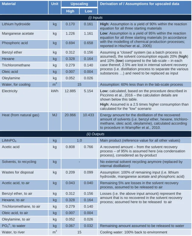
Table S.5 Input and output data for the pilot production of LiMnPO4
Material Unit Upscaling Derivation of / Assumptions for upscaled data High Low
(i) Inputs
Lithium hydroxide kg 0.170 0.161 High: Assumption is a yield of 90% within the reaction
equation for all three starting materials
Low: Assumption is a yield of 95% within the reaction
equation for all three starting materials (in accordance with the modelling of chemical production processes; reported in Hischier et al., 2005)
Manganese acetate kg 1.226 1.161
Phosphoric acid kg 0.694 0.658
Benzyl ether kg 0.312 0.156 Assuming a “closed” system (as a batch process is assumed), the solvent consumption equals 20% (high) and 10% (low) compared to the lab-scale – in each case thereof, 2.5% are lost in internal solvent recovery process (i.e. distillation process to separate the various substances …) and need to be replaced as input
Hexane kg 0.328 0.164
Trichloromethane kg 0.279 0.140
Oleic acid kg 0.007 0.004
Oleylamine kg 0.052 0.026
Water, for cooling m3 15 Assumption: 60% less than in the lab-scale process Electricity kWh 12.885 5.154 Low: calculated, based on the procedure described in
Piccinno et al., 2016 – the calculation details are shown below this table.
High: Assumed is a 2.5 times higher consumption than
calculated for the “low” scenario
Heat (from natural gas) MJ 20.866 10.433 Energy amount for the distillation of the recovered amount of solvents (i.e. benzyl ether, hexane, trichloro-methane, oleic acid, oleylamine), calculated according to procedure in Wampfler et al., 2010.
(ii) Outputs
LiMnPO4 kg 1.0 Main product (reference value for all other values)
Acetic acid kg 0.808 0.766 A recovered amount – from the solvent recovery process – of 95% is assumed here (via condensation process), considered as by-product
Solvents, to recycling kg - No external solvent recycling anymore (replaced by internal distillation)
Wastes for disposal kg 0.209 0.099 Assumption: 100% of remaining input (i.e. lithium hydroxide, manganese acetate and phosphoric acid) Acetic acid, to air kg 0.043 0.040 Remaining 5% are losses in the solvent recovery
process, assumed to be released to air
Benzyl ether, to air kg 0.312 0.156 Losses (i.e. the above input amount) represent the amount that is no recovered in the solvent recovery process; assumed here to be released to air
Hexane, to air kg 0.328 0.164
Trichloromethane, to air kg 0.279 0.140
Oleic acid, to air kg 0.007 0.004
Oleylamine, to air kg 0.052 0.026
PO34-, to water kg 0.067 0.032 Remaining amount assumed to be released to water
Calculation procedure (Piccinno et al., 2016) for estimation of the electricity consumption:
(i) HEATING
Specific heat capacity Cp 1.557 J/g/K Cp of the main solvent used (here 1:1 mix of benzyl
ether and hexane !)
Mass of reaction mixture mmix 2.468 kg sum of input materials & solvents
Reaction temperature T 553.15 K equal to280°C (heating temperature according to input from NH. Kwon)
Reaction time t 2.5 hour process needs to be kept on this temperature for whole reaction time
--> HEATING ENERGY INPUT Qheat 11.414 MJ
(ii) CENTRIFUGE (= Mixing, as process goes over a long period of 3.5 hours)
Density of reaction mixture pmix 1.495 kg/L calculated from individual substances [kg/L] [kg] (data listed below)
Lithium hydroxide 1.46 0.161 Manganese acetate 1.74 1.161 Phosphoric acid 1.89 0.658 Benzyl ether 1.047 0.156 Hexane 0.6606 0.164 Trichloromethane 1.49 0.140 Oleic acid 0.894 0.004 Oleylamine 0.828 0.026
Reaction time t 3.5 hour
-->MIXING ENERGY INPUT Qstir 0.339 MJ
(iii) LIGAND EXCHANGE (= HEATING)
Specific heat capacity Cp 1.557 J/g/K Cp of the main solvent used (see step i)
Mass of reaction mixture mmix 2.468 kg sum of input materials & solvents (see step i)
Reaction temperature T 353.15 K equal to 80°C (heating temperature according to input from NH. Kwon)
Reaction time t 6 hour process needs to be kept on this temperature for whole reaction time
--> HEATING ENERGY INPUT Qheat 5.514 MJ
(iv) DRYING (= HEATING)
Specific heat capacity Cp 1.557 J/g/K Cp of the main solvent used (see step i)
Mass of reaction mixture mmix 2.468 kg sum of input materials & solvents (see step i)
Reaction temperature T 333.15 K equal to 60°C (input NH. Kwon)
Reaction time t 2 hour process needs to be kept on this temperature for whole reaction time
--> HEATING ENERGY INPUT Qheat 1.289 MJ
--> TOTAL ENERGY CONSUMPTION 18.556 MJ resp. 5.154 kWh
3. (BACKGROUND) LIFE CYCLE INVENTORY DATASETS
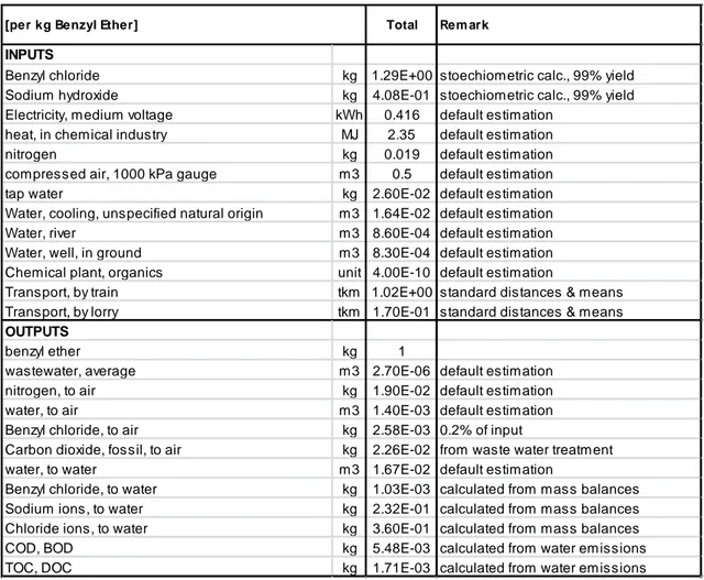
3.1. Benzyl ether
Benzyl ether ((C6H5CH2)2O, CAS-No. 103-50-4) is at room temperature a colourless to pale-yellow
liquid with a boiling point around 298°C (see e.g. www.chemicalbook.com). According to Joshi et al., 1999, there exists several different routes for the synthesis of benzyl ether. The most conventional among these processes is the so-called “Wiliamson’s synthesis”, i.e. the reaction of benzyl chloride with sodium benzylate (NaOCH2Ph) – reaction that has however been adapted by Joshi et al., 1999,
to the following reaction equation, which is modelled here:
2 (C6H5)CH2Cl + 2 NaOH --> (C6H5)CH2)2O + 2 NaCl + H2O
The whole process is modelled here in accordance with the modelling principle for “weak documented chemicals” from Hischier et al., 2005. An overall efficiency of the process of 99% as reported in Joshi et al., 1999, is assumed here – and the amount of the various starting materials is calculated, based on this yield. Heat, electricity, compressed air, nitrogen and water consumption values, as well as transport efforts and infrastructure are modelled with default values (according to procedure in Hischier et al., 2005 – using updated values, collected and calculated by the ecoinvent Centre, 2017). Table S.6 summarizes the resulting input and output values, used to calculate the production of 1 kg of benzyl ether.
Table S.6 Input and output data for the production of 1 kg of benzyl ether
INPUTS
Benzyl chloride kg 1.29E+00 stoechiometric calc., 99% yield Sodium hydroxide kg 4.08E-01 stoechiometric calc., 99% yield Electricity, medium voltage kWh 0.416 default estimation
heat, in chemical industry MJ 2.35 default estimation
nitrogen kg 0.019 default estimation
compressed air, 1000 kPa gauge m3 0.5 default estimation
tap water kg 2.60E-02 default estimation
Water, cooling, unspecified natural origin m3 1.64E-02 default estimation
Water, river m3 8.60E-04 default estimation
Water, well, in ground m3 8.30E-04 default estimation Chemical plant, organics unit 4.00E-10 default estimation
Transport, by train tkm 1.02E+00 standard distances & means Transport, by lorry tkm 1.70E-01 standard distances & means
OUTPUTS
benzyl ether kg 1
wastewater, average m3 2.70E-06 default estimation
nitrogen, to air kg 1.90E-02 default estimation
water, to air m3 1.40E-03 default estimation
Benzyl chloride, to air kg 2.58E-03 0.2% of input
Carbon dioxide, fossil, to air kg 2.26E-02 from waste water treatment
water, to water m3 1.67E-02 default estimation
Benzyl chloride, to water kg 1.03E-03 calculated from mass balances Sodium ions, to water kg 2.32E-01 calculated from mass balances Chloride ions, to water kg 3.60E-01 calculated from mass balances
COD, BOD kg 5.48E-03 calculated from water emissions
TOC, DOC kg 1.71E-03 calculated from water emissions
For the emission side, 0.2% of the input amount of benzyl chloride is assumed to be “emitted to air” while the remaining part goes as part of the waste water flow into the waste water treatment plant (WWTP). There, 90% of this amount is digested and transformed into carbon dioxide (emitted into air) and chloride respectively, the latter leaving the system in their ionic form as a respective release into water. The remaining 10% pass the WWTP and thus are accounted as the release of benzyl chloride into water. All the produced NaCl is assumed to leave the system as release to the water – while sodium hydroxide on the input side is added in excess quantities, assuming a complete (material) recovery of the non-reacting part. According to the description in Hischier et al., 2005, COD, BOD, TOC and DOC values are estimated from the releases in the treated waste water. For their calculation, a worst-case scenario of BOD = COD and TOC = DOC was used.
3.2. Cobalt chloride
According to Wikipedia (Wikipedia Contributors, 2015), cobalt(II) chloride is an inorganic compound of cobalt and chlorine, with the formula CoCl2. It is usually supplied as the hexahydrate CoCl2•6H2O, one
of the most commonly used cobalt compounds in the lab. The hexahydrate is deep purple in colour, whereas the anhydrous form is sky blue. Cobalt chloride has been classified as a substance of very high concern by the European Chemicals Agency (ECA) as it is a suspected carcinogen. According to the information given in Majeau-Bettez et al., 2011, cobalt chloride is produced out of cobalt hydroxide according to the following stoichiometric equation:
Co(OH)2+ 2 HCl → CoCl2•6(H2O)
Also in this case, the whole process is modelled in accordance with the modelling principle for “weak documented chemicals” from Hischier et al., 2005, i.e. an overall efficiency of the process of 95% is assumed – and the amount of starting materials is calculated, based on this yield. Heat, electricity, compressed air, nitrogen and water consumption values, as well as transport efforts and infrastructure are modelled with default values (according to procedure in Hischier et al., 2005 – using updated values, collected and calculated by the ecoinvent Centre, 2017). For the emission side, 0.2% of the two starting materials are assumed to be emitted to air, the remaining part goes as part of the waste water flow into the waste water treatment plant (WWTP) like described in Hischier et al., 2005. There, cobalt ions are bound to 50% in the sludge, while the other 50% are released to nature. The Cl-ions are assumed to be released from the WWTP to 100% in their ionic form. Table S.7 summarizes the resulting input and output values, used to calculate the production of 1 kg of cobalt chloride.
Table S.7 Input and output data for the production of 1 kg of cobalt chloride
INPUTS
Cobalt hydroxide kg 7.54E-01 stoechiometric calc., 95% yield Hydrochloric acid kg 5.91E-01 stoechiometric calc., 95% yield Electricity, medium voltage kWh 0.416 default estimation
heat, in chemical industry MJ 2.35 default estimation
nitrogen kg 0.019 default estimation
compressed air, 1000 kPa gauge m3 0.5 default estimation
tap water kg 2.60E-02 default estimation
Water, cooling, unspecified natural origin m3 1.64E-02 default estimation
Water, river m3 8.60E-04 default estimation
Water, well, in ground m3 8.30E-04 default estimation Chemical plant, organics unit 4.00E-10 default estimation
Transport, by train tkm 8.07E-01 standard distances & means Transport, by lorry tkm 1.34E-01 standard distances & means
OUTPUTS
Cobalt chloride, at plant kg 1
wastewater, average m3 2.70E-06 default estimation
nitrogen, to air kg 1.90E-02 default estimation
water, to air m3 1.40E-03 default estimation
Cobalt hydroxide, to air kg 1.51E-03 0.2% of input Hydrochloric acid, to air kg 1.18E-03 0.2% of input
water, to water m3 1.67E-02 default estimation
Cobalt ions, to water kg 1.15E-02 calculated from mass balances Chloride ions, to water kg 2.76E-02 calculated from mass balances
[per kg Cobalt Chloride] Total Rem ark
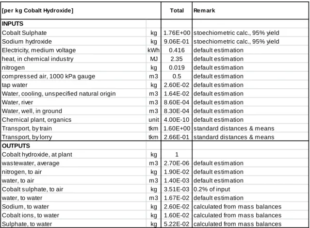
3.3. Cobalt hydroxide
Cobalt hydroxide, the starting material used in the production of cobalt chloride has to be modelled in a similar way due to the fact that a dataset for this substance doesn’t exist neither in the database. According to Majeau-Bettez et al., 2011, cobalt hydroxide could be produced out of cobalt sulphate:
CoSO4+ 2 NaOH → Co(OH)2 + Na2SO4
Again, the entire process is modelled according to the modelling principle for “weak documented chemicals” reported in Hischier et al., 2005, i.e. an overall efficiency of the process of 95% is assumed – and the amount of starting materials is calculated, based on this yield. Heat, electricity, compressed air, nitrogen and water consumption values, as well as transport efforts and infrastructure are modelled with default values (according to procedure in Hischier et al., 2005 – using updated values, collected and calculated by the ecoinvent Centre, 2017). For the emission side, 0.2% of the cobalt-containing starting material is assumed to be emitted to air, the remaining part goes as part of the waste water flow into the waste water treatment plant (WWTP). There, cobalt ions are bound to 50% in the sludge, while the other 50% are released to nature. The sulphate ions are assumed to be released from the WWTP to 100% in their ionic form. The excess sodium hydroxide goes 100% to the WWTP, and leaves in its ionic form (i.e. as sodium ions) the plant in the release to (river) water. The Table S.8 summarizes the resulting input and output values, used to calculate the production of 1 kg of cobalt hydroxide.
Table S.8 Input and output data for the production of 1 kg of cobalt hydroxide
INPUTS
Cobalt Sulphate kg 1.76E+00 stoechiometric calc., 95% yield Sodium hydroxide kg 9.06E-01 stoechiometric calc., 95% yield Electricity, medium voltage kWh 0.416 default estimation
heat, in chemical industry MJ 2.35 default estimation
nitrogen kg 0.019 default estimation
compressed air, 1000 kPa gauge m3 0.5 default estimation
tap water kg 2.60E-02 default estimation
Water, cooling, unspecified natural origin m3 1.64E-02 default estimation
Water, river m3 8.60E-04 default estimation
Water, well, in ground m3 8.30E-04 default estimation Chemical plant, organics unit 4.00E-10 default estimation
Transport, by train tkm 1.60E+00 standard distances & means Transport, by lorry tkm 2.66E-01 standard distances & means
OUTPUTS
Cobalt hydroxide, at plant kg 1
wastewater, average m3 2.70E-06 default estimation
nitrogen, to air kg 1.90E-02 default estimation
water, to air m3 1.40E-03 default estimation
Cobalt sulphate, to air kg 3.51E-03 0.2% of input
water, to water m3 1.67E-02 default estimation
Sodium, to water kg 2.60E-02 calculated from mass balances Cobalt ions, to water kg 1.60E-02 calculated from mass balances Sulphate, to water kg 5.22E-02 calculated from mass balances
[per kg Cobalt Hydroxide] Total Rem ark
3.4. Lithium alkoxides and aryloxides
According to Bradley et al., 2001, and Turova et al., 2002, alkoxides are conjugate bases of an alcohol and consist of an organic group bonded to a negatively charged oxygen atom. They can be written as RO−, where R is the organic substituent. Alkoxides are strong bases and, when R is not bulky, good nucleophiles and good ligands. Alkoxides can be produced by several routes starting from an alcohol. Highly reducing metals react directly with alcohols to give the corresponding metal alkoxide.
The formation reactions for the different types of lithium alkoxides and lithium aryloxides taken into account here are the following:
Lithium methoxide pathway: 2 Li + 2 CH3OH → 2 CH3OLi + H2
Lithium ethoxide pathway: 2 Li + 2 C2H5OH → 2 C2H5OLi + H2
Lithium isopropoxide pathway: 2 Li + 2 C3H7OH → 2 C3H7OLi + H2
Lithium tert-butoxide pathway: 2 Li + 2 C4H9OH → 2 C4H9OLi + H2
Lithium phenoxide pathway: 2 Li + 2 C6H5OH → 2 C6H5OLi + H2
Again, all processes are modelled with the support of the modelling principle for “weak documented chemicals” reported in Hischier et al., 2005. For the above reactions, an overall efficiency of the process of 90%, as reported in the process description published in Talalaeva et al., 1964, is used here. The amount of the various starting materials is then calculated based on this yield. Heat, electricity, compressed air, nitrogen and water consumption values, as well as transport efforts and
updated values, collected and calculated by the ecoinvent Centre, 2017). Concerning the emissions and releases, all excess lithium is assumed to leave the system in ionic form as release into water (i.e. to pass via the WWTP). From the various (starting) alcohols 0.2% of the initial amounts are assumed to be emitted to air, the remaining part goes as part of the waste water flow into the waste water treatment plant (WWTP) like described in Hischier et al., 2005. There, 90% of this amount is digested and transformed into carbon dioxide (emitted into air). The remaining 10% pass the WWTP and thus are accounted as release of the respective alcohol into water. According to the description in Hischier et al., 2005, COD, BOD, TOC and DOC values are estimated from the releases in the treated waste water. For their calculation, a worst-case scenario of BOD = COD and TOC = DOC was used. Table S.9 to Table S.13 summarize the resulting input and output values, used to calculate the production of 1 kg of the various lithium alkoxides and lithium aryloxides taken into account here.
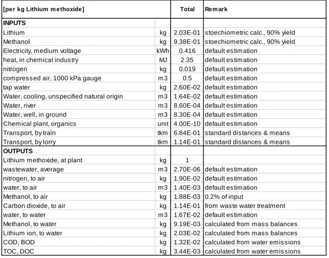
Table S.9 Input and output data for the production of 1 kg of lithium methoxide
INPUTS
Lithium kg 2.03E-01 stoechiometric calc., 90% yield
Methanol kg 9.38E-01 stoechiometric calc., 90% yield
Electricity, medium voltage kWh 0.416 default estimation heat, in chemical industry MJ 2.35 default estimation
nitrogen kg 0.019 default estimation
compressed air, 1000 kPa gauge m3 0.5 default estimation
tap water kg 2.60E-02 default estimation
Water, cooling, unspecified natural origin m3 1.64E-02 default estimation
Water, river m3 8.60E-04 default estimation
Water, well, in ground m3 8.30E-04 default estimation Chemical plant, organics unit 4.00E-10 default estimation
Transport, by train tkm 6.84E-01 standard distances & means Transport, by lorry tkm 1.14E-01 standard distances & means
OUTPUTS
Lithium methoxide, at plant kg 1
wastewater, average m3 2.70E-06 default estimation
nitrogen, to air kg 1.90E-02 default estimation
water, to air m3 1.40E-03 default estimation
Methanol, to air kg 1.88E-03 0.2% of input
Carbon dioxide, to air kg 1.14E-01 from waste water treatment
water, to water m3 1.67E-02 default estimation
Methanol, to water kg 9.19E-03 calculated from mass balances Lithium ion, to water kg 2.03E-02 calculated from mass balances
COD, BOD kg 1.32E-02 calculated from water emissions
TOC, DOC kg 3.44E-03 calculated from water emissions
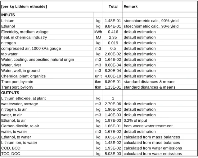
Table S.10 Input and output data for the production of 1 kg of lithium ethoxide
INPUTS
Lithium kg 1.48E-01 stoechiometric calc., 90% yield
Ethanol kg 9.84E-01 stoechiometric calc., 90% yield
Electricity, medium voltage kWh 0.416 default estimation heat, in chemical industry MJ 2.35 default estimation
nitrogen kg 0.019 default estimation
compressed air, 1000 kPa gauge m3 0.5 default estimation
tap water kg 2.60E-02 default estimation
Water, cooling, unspecified natural origin m3 1.64E-02 default estimation
Water, river m3 8.60E-04 default estimation
Water, well, in ground m3 8.30E-04 default estimation Chemical plant, organics unit 4.00E-10 default estimation
Transport, by train tkm 6.80E-01 standard distances & means Transport, by lorry tkm 1.13E-01 standard distances & means
OUTPUTS
Lithium ethoxide, at plant kg 1
wastewater, average m3 2.70E-06 default estimation
nitrogen, to air kg 1.90E-02 default estimation
water, to air m3 1.40E-03 default estimation
Ethanol, to air kg 1.97E-03 0.2% of input
Carbon dioxide, to air kg 1.66E-01 from waste water treatment
water, to water m3 1.67E-02 default estimation
Ethanol, to water kg 9.65E-03 calculated from mass balances Lithium ion, to water kg 1.48E-02 calculated from mass balances
COD, BOD kg 1.93E-02 calculated from water emissions
TOC, DOC kg 5.03E-03 calculated from water emissions
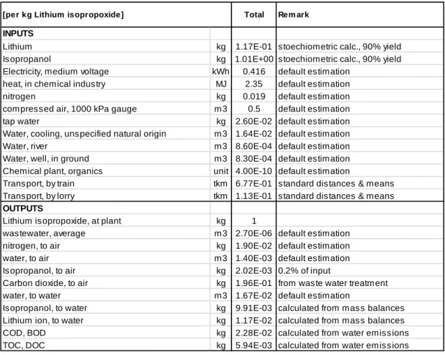
Table S.11 Input and output data for the production of 1 kg of lithium isopropoxide
INPUTS
Lithium kg 1.17E-01 stoechiometric calc., 90% yield
Isopropanol kg 1.01E+00 stoechiometric calc., 90% yield Electricity, medium voltage kWh 0.416 default estimation
heat, in chemical industry MJ 2.35 default estimation
nitrogen kg 0.019 default estimation
compressed air, 1000 kPa gauge m3 0.5 default estimation
tap water kg 2.60E-02 default estimation
Water, cooling, unspecified natural origin m3 1.64E-02 default estimation
Water, river m3 8.60E-04 default estimation
Water, well, in ground m3 8.30E-04 default estimation Chemical plant, organics unit 4.00E-10 default estimation
Transport, by train tkm 6.77E-01 standard distances & means Transport, by lorry tkm 1.13E-01 standard distances & means
OUTPUTS
Lithium isopropoxide, at plant kg 1
wastewater, average m3 2.70E-06 default estimation
nitrogen, to air kg 1.90E-02 default estimation
water, to air m3 1.40E-03 default estimation
Isopropanol, to air kg 2.02E-03 0.2% of input
Carbon dioxide, to air kg 1.96E-01 from waste water treatment
water, to water m3 1.67E-02 default estimation
Isopropanol, to water kg 9.91E-03 calculated from mass balances Lithium ion, to water kg 1.17E-02 calculated from mass balances
COD, BOD kg 2.28E-02 calculated from water emissions
TOC, DOC kg 5.94E-03 calculated from water emissions
Table S.12 Input and output data for the production of 1 kg of lithium tert-butoxide
INPUTS
Lithium kg 9.63E-02 stoechiometric calc., 90% yield
Tert-butanol kg 1.03E+00 stoechiometric calc., 90% yield Electricity, medium voltage kWh 0.416 default estimation
heat, in chemical industry MJ 2.35 default estimation
nitrogen kg 0.019 default estimation
compressed air, 1000 kPa gauge m3 0.5 default estimation
tap water kg 2.60E-02 default estimation
Water, cooling, unspecified natural origin m3 1.64E-02 default estimation
Water, river m3 8.60E-04 default estimation
Water, well, in ground m3 8.30E-04 default estimation Chemical plant, organics unit 4.00E-10 default estimation
Transport, by train tkm 6.75E-01 standard distances & means Transport, by lorry tkm 1.13E-01 standard distances & means
OUTPUTS
Lithium tert-butoxide, at plant kg 1
wastewater, average m3 2.70E-06 default estimation
nitrogen, to air kg 1.90E-02 default estimation
water, to air m3 1.40E-03 default estimation
Tert-butanol, to air kg 2.06E-03 0.2% of input
Carbon dioxide, to air kg 2.16E-01 from waste water treatment
water, to water m3 1.67E-02 default estimation
Tert-butanol, to water kg 1.01E-02 calculated from mass balances Lithium ion, to water kg 9.63E-03 calculated from mass balances
COD, BOD kg 2.51E-02 calculated from water emissions
TOC, DOC kg 6.53E-03 calculated from water emissions
Table S.13 Input and output data for the production of 1 kg of lithium phenoxide
INPUTS
Lithium kg 7.71E-02 stoechiometric calc., 90% yield
Phenol kg 1.05E+00 stoechiometric calc., 90% yield
Electricity, medium voltage kWh 0.416 default estimation heat, in chemical industry MJ 2.35 default estimation
nitrogen kg 0.019 default estimation
compressed air, 1000 kPa gauge m3 0.5 default estimation
tap water kg 2.60E-02 default estimation
Water, cooling, unspecified natural origin m3 1.64E-02 default estimation
Water, river m3 8.60E-04 default estimation
Water, well, in ground m3 8.30E-04 default estimation Chemical plant, organics unit 4.00E-10 default estimation
Transport, by train tkm 6.73E-01 standard distances & means Transport, by lorry tkm 1.12E-01 standard distances & means
OUTPUTS
Lithium tert-butoxide, at plant kg 1
wastewater, average m3 2.70E-06 default estimation
nitrogen, to air kg 1.90E-02 default estimation
water, to air m3 1.40E-03 default estimation
Phenol, to air kg 2.09E-03 0.2% of input
Carbon dioxide, to air kg 2.59E-01 from waste water treatment
water, to water m3 1.67E-02 default estimation
Phenol, to water kg 1.02E-02 calculated from mass balances Lithium ion, to water kg 7.71E-03 calculated from mass balances
COD, BOD kg 2.33E-02 calculated from water emissions
TOC, DOC kg 7.81E-03 calculated from water emissions
[per kg Lithium phenoxide] Total Rem ark
3.5. Oleylamine
According to the respective Toxic Substance Control Act (TSCA) annex (US-EPA, 1986) Oleylamine, or 9-octadecenylamine (ODA, CAS No. 112-90-3) is a yellow liquid with an ammoniacal odour. It has very low volatility and water solubility although water is soluble in it. It is miscible with a variety of organic solvents. Within this project, ODA has been synthesised by the authors in the following way: • To a 5-litre flange neck flask fitted with overhead stirrer, temperature probe, nitrogen inlet and a
500 cm3 dropping funnel was charged oleic acid (400 g, 1.416 mol) and dichloromethane (3.20 L). The resultant solution was heated to reflux (39-41°C) and thionyl chloride (202.4 g, 1.2 eq.) added over 10 minutes between 39-41°C.
• The reaction mixture was heated at reflux for 3 hours, sampling the mixture at hourly intervals (sample quenched into anhydrous methanol, shaken well, and stored at ambient for >1 hour before submitted to analytical development for analysis). The reaction was shown to be 99.9% complete after 3 hours. As the reaction mixture was used in the subsequent amidation reaction without delay, no isomerisation to the trans-isomer was observed.
• To a 20-litre flange-neck flask fitted with overhead stirrer, nitrogen inlet, condenser (with silica drying tube) and a gas sparging inlet was charged dichloromethane (12.00 Kg, ~9.1 L). The solvent was cooled to 0-10 °C and then ammonia (960 g) was charged as a gas via the sparging inlet over 140 minutes, maintaining the reaction mixture between 0-10°C. The acid chloride
500 cm3 dropping funnel over 32 minutes, maintaining the reaction temperature below 20°C. The resultant pink-coloured suspension could be stirred at ambient temperature overnight. A sample was taken (sample quenched into methanol). The resulting reaction mixture was shown to be 76.69% oleylamide and 22.53% oleic acid.
For the calculations here, dichloromethane and thionyl chloride are assumed to have a catalytic role (i.e. don’t react during the above described procedure) and therefore, the above described process is simplified here with the stoichiometric equation:
C18H34O2 (Oleic acid) + NH3 → C18H35NH2 + O2
Again, this process is modelled here according to the modelling principle for “weak documented chemicals” reported in Hischier et al., 2005, using the above reported efficiency for the oleic acid transformation of 77%. For the further inputs, the default yield of 95% is used in order to calculate the related input amounts. Heat, electricity, compressed air, nitrogen and water consumption values, as well as transport efforts and infrastructure are modelled with default values (according to procedure in Hischier et al., 2005 – using updated values, collected and calculated by the ecoinvent Centre, 2017).
Table S.14 Input and output data for the production of 1 kg of oleylamine
INPUTS
Oleic acid kg 1.09E+00 stoechiometric calc., 77% yield, 90% of exess to WWTP recovered
Ammonia kg 6.70E-02 stoechiometric calc., 95% yield
Electricity, medium voltage kWh 0.416 default estimation heat, in chemical industry MJ 2.35 default estimation
nitrogen kg 0.019 default estimation
compressed air, 1000 kPa gauge m3 0.5 default estimation
tap water kg 2.60E-02 default estimation
Water, cooling, unspecified natural origin m3 1.64E-02 default estimation
Water, river m3 8.60E-04 default estimation
Water, well, in ground m3 8.30E-04 default estimation Chemical plant, organics unit 4.00E-10 default estimation
Transport, by train tkm 8.63E-01 standard distances & means Transport, by lorry tkm 1.44E-01 standard distances & means
OUTPUTS
Ooleylamine kg 1
wastewater, average m3 2.70E-06 default estimation
nitrogen, to air kg 1.90E-02 default estimation
water, to air m3 1.40E-03 default estimation
Oleic acid, to air kg 2.74E-03 0.2% of input
Ammonia, to air kg 1.34E-04 0.2% of input
carbon dioxide, fossil, to air kg 7.89E-02 from waste water treatment
water, to water m3 1.67E-02 default estimation
Oleic acid, to water kg 3.13E-03 calculated from mass balances Ammonium, to water kg 9.65E-04 calculated from WWTP model Nitrate, to water kg 2.21E-03 calculated from WWTP model
COD, BOD kg 1.48E-02 calculated from water emissions
TOC, DOC kg 4.08E-03 calculated from water emissions
For the emission side, 0.2% of the starting materials (i.e. oleic acid and ammonia) are assumed to be emitted to air, the remaining part goes as part of the waste water flow into the waste water treatment plant (WWTP) like described in Hischier et al., 2005. 90% of this remaining oleic acid amount is recovered as oleic acid (… and thus deducted from the overall input amount here) while the remaining 10% goes into the WWTP process. Here, 90% are digested and transformed into carbon dioxide (emitted into air), while the remaining 10% pass the WWTP and thus are accounted as release into water. For ammonia, a removal efficiency for NH4-N of 70% and for total N of 50% was assumed. The
remaining emissions to water were considered as ammonium (NH4) and nitrate (NO3). The nitrogen
emitted to air (N2) and remaining in the sewage sludge was neglected. Table S.14 summarizes the
resulting input and output values, used in this study to calculate the production efforts from 1 kg of oleylamine.
3.6. Manganese acetate
Anhydrous manganese(II) acetate (Mn(CH3COO)2, CAS No. 638-38-0) is a pale pink crystal solid at
room temperature. It is soluble in water, methanol, acetic acid (Wikipedia Contributors, 2015). In the PhD thesis of Dai (Dai, 2014), the production pathway from manganese oxide (Mn2O3) – for which a
respective dataset can be found in ecoinvent – to manganese(II) acetate, via the intermediates manganese sulphate and manganese carbonate, is reported in a simplified way. These reported datasets are used in this study.
3.7. Solvent recycling
In research institutions like e.g. University of Fribourg, all the liquid chemical waste is collected at the working places via collecting drums, distinguishing usually between halogenated organic solvents, halogen-free organic solvents as well as aqueous solutions of salts and heavy metals1. These drums are going to specialist companies for the further treatment of such waste. In his PhD thesis (Capello, 2006), Capello has analysed statistically the data of more than 100 waste solvent distillation processes in the chemical industry. In Capello et al., 2005, the resulting inventory data for this (average) waste solvent distillation process are reported – data that have been used here as model for the “default” situation of the treatment of waste solvent flows.
Table S.15 summarizes the various inputs and outputs of this recycling process.
Table S.15 Input and output data for the treatment of 1 kg of (used) solvents
INPUTS
Waste solvent, for treatement kg 1
Water, cooling, unspecified natural origin m3 2.70E-02 Capello et al. 2005
Electricity, medium voltage kWh 3.00E-02 Capello et al. 2005
Steam, in chemical industry kg 1.40E+00 Capello et al. 2005
Nitrogen, liquid kg 1.50E-03 Capello et al. 2005
transport, by lorry (7.5-16t) tkm 2.00E-01 Capello et al. 2005
OUTPUTS
recycled solvent kg 7.10E-01 Capello et al. 2005
solvent, to hazardous waste incinerator kg 2.90E-01 Capello et al. 2005
BENEFITS from hazardous waste treatment
Electricity, high voltage kWh 4.96E+00
Heat, from natural gas MJ 1.84E-01
Heat, from light fuel oil MJ 1.84E-01
[per kg solvent entering the recycling process] Total Rem ark
calculated, based on default values in applied ecoinvent dataset (Doka, 2007)
Doka, 2007
4. RESULTS OF LCA-CALCULATIONS
4.1. Lab-Scale
Numerical LCA results for the production of 1 kg of cathode in case of the nano-structured LiCoO2 (i.e.
values shown in Figure 2 of the manuscript):
LiCoO2 Composite Electrode Al-Foil Fossil depletion FDP kg oil eq 1.61E+01 6.31E-01 1.55E+00 3.26E+00 Metal depletion MDP kg Fe eq 2.78E+00 3.46E-01 2.44E-01 3.02E-01 Climate Change GWP kg CO2 eq 5.69E+01 2.05E+00 1.16E+01 1.53E+01 Terrestrial acidification TAP kg SO2 eq 2.70E-01 7.27E-03 3.06E-02 1.22E-01 Freshwater eutrophication FEP kg P eq 2.69E-02 1.45E-03 3.93E-03 4.68E-03 Particulate matter formation PMFP kg PM10 eq 9.79E-02 3.01E-03 1.06E-02 4.33E-02 Photochemical oxidant formation POFP kg NMVOC 3.52E-01 5.01E-03 2.49E-02 5.92E-02 Human toxicity HTP kg 1,4-DB eq 2.76E+01 1.71E+00 2.10E+00 5.58E+00 Freshwater ecotoxicity FETP kg 1,4-DB eq 1.56E+00 2.66E-01 1.36E-01 2.00E-01 Marine ecotoxicity METP kg 1,4-DB eq 1.25E+00 2.34E-01 1.26E-01 1.92E-01
Numerical LCA results for the lab-scale production of 1 kg of LCO nanomaterial (i.e. values shown in Figure 3, upper part, of the manuscript):
GWP FDP FETP FEP HTP METP MDP PMFP POFP TAP
lithium methoxide 1.64E+01 4.82E+00 2.96E-01 1.10E-02 9.33E+00 2.82E-01 9.58E-01 4.26E-02 5.75E-02 1.02E-01 cobalt chloride 1.52E+01 3.49E+00 1.38E+00 4.51E-03 3.37E+01 1.49E+00 4.26E+00 8.32E-02 1.20E-01 1.20E-01 tetrahydrofurane 8.28E+01 3.11E+01 1.04E+00 2.24E-02 2.72E+01 9.06E-01 4.68E+00 1.66E-01 2.90E-01 5.03E-01 methanol 2.19E+00 2.61E+00 3.76E-02 4.10E-04 8.67E-01 1.98E-02 1.21E-01 6.02E-03 1.04E-02 2.40E-02 nitrogen 1.46E+02 4.13E+01 2.82E+00 1.09E-01 8.00E+01 2.63E+00 3.97E+00 1.94E-01 3.08E-01 5.87E-01 argon 8.52E+00 2.25E+00 1.01E-01 3.48E-03 2.81E+00 9.16E-02 1.36E-01 1.90E-02 2.51E-02 5.07E-02 water 4.34E-01 1.15E-01 1.77E-02 1.80E-04 2.33E-01 1.62E-02 3.65E-02 1.03E-03 1.42E-03 2.58E-03 electricity 1.27E+01 3.83E+00 1.70E+00 8.93E-03 1.08E+01 1.49E+00 2.22E+00 1.74E-02 2.83E-02 4.39E-02 solvent recycling 2.11E+01 -2.45E+00 1.05E+00 -1.43E-02 -1.62E+01 -2.04E-01 -1.37E+00 -8.40E-04 1.76E-02 2.59E-02 waste treatment 3.91E-01 3.66E-02 3.22E-03 1.30E-04 5.57E-02 3.09E-03 4.71E-03 3.00E-04 7.70E-04 8.50E-04 direct releases 1.44E+00 0.00E+00 9.85E-05 0.00E+00 4.52E-01 3.03E-03 0.00E+00 5.14E-06 1.04E+00 8.36E-08
Numerical LCA results for the lab-scale production of 1 kg of LMP nanomaterial (i.e. values shown in Figure 3, lower part, of the manuscript):
GWP FDP FETP FEP HTP METP MDP PMFP POFP TAP
lithium hydroxide 2.07E+00 5.24E-01 3.49E-02 1.27E-03 9.87E-01 3.31E-02 1.81E-01 4.47E-03 7.97E-03 1.24E-02 manganese acetate 4.90E+00 1.87E+00 9.01E-02 1.96E-03 2.29E+00 8.27E-02 4.78E+01 1.02E-02 1.82E-02 3.03E-02 phosphoric acid 7.49E-01 3.11E-01 3.12E-02 1.47E-03 7.12E-01 3.05E-02 1.21E-01 3.47E-03 4.11E-03 1.03E-02 benzyl ether 8.15E+01 3.89E+01 1.00E+00 2.12E-02 3.18E+01 1.01E+00 4.74E+00 1.31E-01 2.86E-01 3.56E-01 oleylamine 1.61E+01 1.77E+00 1.56E-01 2.99E-03 2.76E+00 1.13E-01 7.70E-01 2.39E-02 3.65E-02 4.68E-02 oleic acid 1.66E+00 1.25E-01 1.47E-02 2.90E-04 2.24E-01 9.43E-03 6.80E-02 2.43E-03 3.79E-03 4.28E-03 chloroform 5.95E+01 1.23E+01 5.55E-01 1.30E-02 1.18E+02 5.24E-01 2.36E+00 5.21E-02 8.91E-02 1.47E-01 hexane 6.27E+00 8.98E+00 8.60E-02 1.29E-03 2.00E+00 7.79E-02 5.48E-01 1.48E-02 8.32E-02 4.74E-02 electricity 1.84E+02 5.55E+01 2.47E+01 1.30E-01 1.56E+02 2.17E+01 3.22E+01 2.53E-01 4.11E-01 6.38E-01 solvent recycling 6.94E+01 -8.09E+00 3.45E+00 -4.72E-02 -5.34E+01 -6.71E-01 -4.51E+00 -2.76E-03 5.80E-02 8.53E-02 waste treatment 8.12E-02 7.61E-03 6.70E-04 2.76E-05 1.16E-02 6.40E-04 9.80E-04 6.13E-05 1.60E-04 1.80E-04 direct releases 0.00E+00 0.00E+00 3.04E-01 0.00E+00 1.10E-05 1.05E-05 0.00E+00 0.00E+00 2.04E-01 0.00E+00
4.2. (future) Pilot Production
Numerical LCA results for the (theoretical) pilot production of 1 kg of LCO nanomaterial (i.e. values shown in Figure 4, upper part, of the manuscript):
FDP MDP GWP TAP FEP PMFP POFP HTP FETP METP
lithium methoxide 4.38E+00 8.71E-01 1.49E+01 9.23E-02 9.96E-03 3.88E-02 5.23E-02 8.49E+00 2.69E-01 2.57E-01 cobalt chloride 3.30E+00 4.02E+00 1.44E+01 1.13E-01 4.26E-03 7.86E-02 1.14E-01 3.18E+01 1.31E+00 1.41E+00 solvents 2.39E-01 1.68E-02 2.99E-01 2.58E-03 6.79E-05 7.20E-04 1.25E-03 1.09E-01 4.48E-03 2.98E-03 inert gas 1.79E-01 1.72E-02 6.33E-01 2.54E-03 4.70E-04 8.40E-04 1.33E-03 3.46E-01 1.22E-02 1.14E-02 water 2.30E-02 7.31E-03 8.70E-02 5.20E-04 3.53E-05 2.10E-04 2.80E-04 4.67E-02 3.54E-03 3.24E-03 electricity 7.72E-01 4.47E-01 2.55E+00 8.87E-03 1.80E-03 3.51E-03 5.71E-03 2.17E+00 3.43E-01 3.02E-01 heat (natural gas) 9.94E-03 2.70E-04 2.93E-02 5.00E-05 1.25E-06 1.71E-05 6.17E-05 1.19E-03 4.29E-05 3.99E-05 waste treatment 6.61E-02 1.61E-02 6.79E-01 1.64E-03 2.78E-04 5.72E-04 1.42E-03 1.08E-01 6.76E-03 6.40E-03 direct emissions 0.00E+00 0.00E+00 1.35E+00 0.00E+00 3.25E-06 0.00E+00 7.17E-02 6.57E-02 5.31E-06 4.24E-05
Numerical LCA results for the (theoretical) pilot production of 1 kg of LMP nanomaterial (i.e. values shown in Figure 4, lower part, of the manuscript):
FDP MDP GWP TAP FEP PMFP POFP HTP FETP METP
lithium hydroxide 2.21E-01 7.66E-02 8.74E-01 5.23E-03 5.40E-04 1.90E-03 3.40E-03 4.19E-01 1.48E-02 1.41E-02 manganese acetate 1.97E+00 5.03E+01 5.16E+00 3.19E-02 2.07E-03 1.07E-02 1.91E-02 2.41E+00 9.48E-02 8.71E-02 phosphoric acid 4.34E-01 1.69E-01 1.04E+00 1.43E-02 2.05E-03 4.84E-03 5.73E-03 9.91E-01 4.34E-02 4.25E-02 solvents 5.35E-01 7.34E-02 1.43E+00 5.19E-03 3.30E-04 1.94E-03 4.31E-03 1.34E+00 1.57E-02 1.50E-02 electricity 2.18E-01 1.26E-01 7.21E-01 2.50E-03 5.10E-04 9.90E-04 1.61E-03 6.12E-01 9.69E-02 8.51E-02 heat (natural gas) 1.09E-01 3.06E-03 3.21E-01 5.50E-04 1.38E-05 1.80E-04 6.50E-04 1.32E-02 4.80E-04 4.40E-04 waste treatment 2.51E-02 3.23E-03 2.68E-01 5.80E-04 9.10E-05 2.00E-04 5.30E-04 3.82E-02 2.21E-03 2.12E-03 direct emissions 0.00E+00 3.32E-04 4.34E+00 5.37E-05 1.02E-02 0.00E+00 2.07E-01 4.78E+00 4.57E-04 7.53E-03
Numerical relative changes of the result of the (theoretical) pilot production of 1 kg of (LCO, LMP) nanomaterial when changing the various key elements from the lower to the higher value (i.e. values shown in Figure 5 of the manuscript):
FDP MDP GWP TAP FEP PMFP POFP HTP FETP METP
material input 3.43E-02 3.13E-02 3.73E-02 3.41E-02 3.29E-02 3.44E-02 2.63E-02 3.13E-02 3.11E-02 3.11E-02 amount of inert gas 3.45E-03 7.83E-04 3.40E-03 2.49E-03 2.74E-03 1.52E-03 1.29E-03 1.15E-03 5.04E-04 4.91E-04 losses of solvents 1.67E-02 4.10E-03 5.37E-03 6.69E-03 1.37E-03 4.21E-03 2.23E-01 1.88E-03 6.00E-04 4.23E-04 electricity consumption 9.64E-02 1.67E-01 8.73E-02 4.12E-02 6.30E-02 3.30E-02 2.83E-02 5.23E-02 3.01E-02 2.89E-02 material input 4.67E-02 5.59E-02 5.58E-02 5.17E-02 2.32E-02 5.29E-02 1.22E-02 2.23E-02 5.20E-02 4.91E-02 losses of solvents 2.34E-01 1.55E-03 3.05E-01 1.29E-01 3.23E-02 1.29E-01 8.08E-01 5.97E-01 1.12E-01 1.65E-01 electricity consumption 5.93E-02 1.85E-03 6.30E-02 3.39E-02 3.91E-02 3.65E-02 7.39E-03 5.46E-02 1.68E-01 1.58E-01
LCO
LMP
Numerical relative results representing the range of the environmental impact of the (theoretical) pilot production processes for LCO and LMP relative tos the respective lab-scale impacts (set each time 100%) (i.e. values shown in Figure 6 of the manuscript):
FDP MDP GWP TAP FEP PMFP POFP HTP FETP METP
nano LCO, low 5.63E-02 1.41E-01 6.14E-02 8.07E-02 1.19E-01 1.03E-01 5.60E-02 1.83E-01 2.52E-01 2.86E-01 nano LCO, high 1.16E-01 3.04E-01 1.25E-01 1.57E-01 2.36E-01 1.99E-01 1.29E-01 3.58E-01 4.80E-01 5.45E-01 nano LMP, low 2.98E-02 7.22E-01 2.88E-02 5.17E-02 9.24E-02 5.08E-02 1.81E-01 4.92E-02 1.73E-02 2.63E-02 nano LMP, high 4.00E-02 7.65E-01 4.09E-02 6.27E-02 1.62E-01 6.19E-02 3.31E-01 8.24E-02 2.31E-02 3.60E-02
4.3. Comparison with other cathode materials
Numerical LCA results of the impacts for the production of 1 kg of various Li-containing cathode materials (i.e. values shown in Figure 7 of the manuscript):
Unit
nano-LiCoO2 LiCoO2 Li-NMC LiFePO4 LiMn2O4
nano-LiMnPO4
fossil depletion - FDP kg oil-Eq 8.78E+00 5.62E+00 2.57E+00 1.72E+00 1.11E+00 3.97E+00
metal depletion - MDP kg Fe-Eq 2.00E+00 1.24E+00 3.22E+01 4.73E-01 7.40E+01 5.07E+01
climate change - GWP100 kg CO2-Eq 3.21E+01 2.12E+01 1.06E+01 5.83E+00 4.32E+00 1.25E+01 terrestrial acidification - TAP100 kg SO2-Eq 1.89E-01 1.37E-01 3.98E-01 3.78E-02 1.81E-02 6.44E-02 freshwater eutrophication - FEP kg P-Eq 3.94E-02 3.09E-02 1.74E-02 4.59E-03 2.21E-03 1.76E-02 particulate matter formation - PMFP kg PM10-Eq 1.07E-01 7.77E-02 1.06E-01 1.56E-02 8.49E-03 2.74E-02 photochemical oxidant formation - POFP kg NMVOC 2.13E-01 1.11E-01 8.05E-02 1.97E-02 1.09E-02 1.95E-01 human toxicity - HTPinf kg 1,4-DCB-Eq 5.62E+01 4.72E+01 2.78E+01 3.39E+00 1.88E+00 1.52E+01 freshwater ecotoxicity - FETPinf kg 1,4-DCB-Eq 4.10E+00 3.74E+00 1.05E+00 9.70E-02 5.37E-02 2.07E-01 marine ecotoxicity - METPinf kg 1,4-DCB-Eq 3.95E+00 3.61E+00 1.02E+00 9.02E-02 4.98E-02 2.05E-01
Numerical LCA results of the impacts for 1 kWh of stored energy for the various Li-containing cathode materials (i.e. values shown in Figure 8, upper part, of the manuscript):
nano-LCO HT-LCO Li-NMC LFP LMO nano-LMP
fossil depletion - FDP kg oil-Eq 2.42E-05 1.24E-05 2.82E-06 2.10E-06 5.03E-06 4.78E-06
metal depletion - MDP kg Fe-Eq 5.51E-06 2.73E-06 3.53E-05 5.80E-07 3.37E-04 6.11E-05
climate change - GWP100 kg CO2-Eq 8.83E-05 4.68E-05 1.16E-05 7.15E-06 1.96E-05 1.50E-05 terrestrial acidification - TAP100 kg SO2-Eq 5.20E-07 3.03E-07 4.36E-07 4.63E-08 8.24E-08 7.75E-08 freshwater eutrophication - FEP kg P-Eq 1.09E-07 6.80E-08 1.91E-08 5.62E-09 1.00E-08 2.12E-08 particulate matter formation - PMFP kg PM10-Eq 2.95E-07 1.71E-07 1.16E-07 1.92E-08 3.86E-08 3.30E-08 photochemical oxidant formation - POFP kg NMVOC 5.88E-07 2.44E-07 8.82E-08 2.41E-08 4.97E-08 2.34E-07 human toxicity - HTPinf kg 1,4-DCB-Eq 1.55E-04 1.04E-04 3.05E-05 4.16E-06 8.53E-06 1.82E-05 freshwater ecotoxicity - FETPinf kg 1,4-DCB-Eq 1.13E-05 8.24E-06 1.15E-06 1.19E-07 2.44E-07 2.50E-07 marine ecotoxicity - METPinf kg 1,4-DCB-Eq 1.09E-05 7.96E-06 1.12E-06 1.11E-07 2.26E-07 2.46E-07
Numerical LCA results of the impacts for 1 Ah of available capacity for the various Li-containing cathode materials (i.e. values shown in Figure 8, lower part, of the manuscript):
nano-LCO HT-LCO Li-NMC LFP LMO nano-LMP
fossil depletion - FDP kg oil-Eq 9.44E-08 5.35E-08 1.07E-08 7.15E-09 2.01E-08 1.96E-08
metal depletion - MDP kg Fe-Eq 2.15E-08 1.18E-08 1.34E-07 1.97E-09 1.35E-06 2.51E-07
climate change - GWP100 kg CO2-Eq 3.45E-07 2.02E-07 4.43E-08 2.43E-08 7.85E-08 6.15E-08 terrestrial acidification - TAP100 kg SO2-Eq 2.03E-09 1.31E-09 1.66E-09 1.57E-10 3.30E-10 3.18E-10 freshwater eutrophication - FEP kg P-Eq 4.24E-10 2.94E-10 7.27E-11 1.91E-11 4.01E-11 8.72E-11 particulate matter formation - PMFP kg PM10-Eq 1.15E-09 7.40E-10 4.43E-10 6.51E-11 1.54E-10 1.35E-10 photochemical oxidant formation - POFP kg NMVOC 2.30E-09 1.06E-09 3.35E-10 8.20E-11 1.99E-10 9.62E-10 human toxicity - HTPinf kg 1,4-DCB-Eq 6.04E-07 4.50E-07 1.16E-07 1.41E-08 3.41E-08 7.48E-08 freshwater ecotoxicity - FETPinf kg 1,4-DCB-Eq 4.41E-08 3.56E-08 4.36E-09 4.04E-10 9.77E-10 1.02E-09 marine ecotoxicity - METPinf kg 1,4-DCB-Eq 4.25E-08 3.44E-08 4.25E-09 3.76E-10 9.05E-10 1.01E-09
5. REFERENCES
Bradley, D. C., et al. (2001). Alkoxo and Aryloxo Derivatives of Metals. San Diego - San Francisco - New York (USA), Academic Press.
Capello, C. (2006). Environmental Assessment of Waste-Solvent Treatment in the Swiss Chemical Industry. Zürich (Switzerland), Swiss Federal Institute of Technology (ETH). Doctor of Natural
Sciences.
Capello, C., et al. (2005). "Life-Cycle Inventory of Waste-Solvent Distillation: Statistical Analysis of Empirical Data." Environmental Science & Technology 39(15): 5885-5892.
Dai, Q. (2014). Life Cycle Assessment of Natural Gas Utilization in Light-duty Passenger Vehicles. Civil and Environmental Engineering Ann Arbor, MI (USA), University of Michigan. PhD (Doctor of
Philosophy): 166.
Doka, G. (2007). Life Cycle Inventories of Waste Treatment Services. Dübendorf, CH, EMPA St. Gallen, Swiss Centre for Life Cycle Inventories.
Hischier, R., et al. (2005). "Establishing Life Cycle Inventories of Chemicals Based on Differing Data Availability." Int J LCA 10(1): 59-67.
Joshi, S. R., et al. (1999). "Process Development Aspects of Production of Dibenzyl Ether." Organic Process Research & Development 3: 17-27.
Majeau-Bettez, G., et al. (2011). "Life Cycle Environmental Assessment of Lithium-Ion and Nickel Metal Hydride Batteries for Plug-In Hybrid and Battery Electric Vehicles." Environmental Science & Technology 45: 4548-4554.
Piccinno, F., et al. (2016). "From laboratory to industrial scale: scale-up calculations for chemical processes in life cycle assessment studies." Journal of Cleaner Production 135: 1085-1097.
Talalaeva, T. V., et al. (1964). "Synthesis and Structure of Soluble Lithium Alkoxides." Izvestiya Akademii Nauk SSSR, Seriya Khimicheskaya 4: 638-644.
Turova, N. Y., et al. (2002). The Chemistry of Metal Alkoxides. New York - Boston - Dordrecht - London - Moscow, Kluwer Academic Publishers.
US-EPA (1986). Assessment of Testing Nees: Oleylamine (9-Octadecnylamine) - Support Document Proposed Health Effects Test Rule, Toxic Substance Control Act, Section 4. Washington D.C. (USA), Existing Chemical Assessment Division, Office of Toxic Substances - US Environmental Protection Agency: 96.
Wampfler, B., et al. (2010). "Isolation and Purification of Medium Chain Length Poly(3-hydroxyalkanoates) (mcl-PHA) for Medical Applications Using Nonchlorinated Solvents." Biomacromolecules 11: 2716-2723.
Wikipedia Contributors (2015). Cobalt(II) chloride. Wikipedia, The Free Encyclopedia, Wikipedia. Wikipedia Contributors (2015). Manganese(II) acetate. Wikipedia, The Free Encyclopedia, Wikipedia.