Foreword iii
Preface v
1. Real Numbers 1
1.1 Introduction 1
1.2 Euclid’s Division Lemma 2
1.3 The Fundamental Theorem of Arithmetic 7
1.4 Revisiting Irrational Numbers 11
1.5 Revisiting Rational Numbers and Their Decimal Expansions 15
1.6 Summary 18
2. Polynomials 2 0
2.1 Introduction 20
2.2 Geometrical Meaning of the Zeroes of a Polynomial 21
2.3 Relationship between Zeroes and Coefficients of a Polynomial 28
2.4 Division Algorithm for Polynomials 33
2.5 Summary 37
3. Pair of Linear Equations in Two Variables 3 8
3.1 Introduction 38
3.2 Pair of Linear Equations in Two Variables 39
3.3 Graphical Method of Solution of a Pair of Linear Equations 44 3.4 Algebraic Methods of Solving a Pair of Linear Equations 50
3.4.1 Substitution Method 50
3.4.2 Elimination Method 54
3.4.3 Cross-Multiplication Method 57
3.5 Equations Reducible to a Pair of Linear Equations in Two Variables 63
3.6 Summary 69
4. Quadratic Equations 7 0
4.1 Introduction 70
4.3 Solution of a Quadratic Equation by Factorisation 74 4.4 Solution of a Quadratic Equation by Completing the Square 76
4.5 Nature of Roots 88 4.6 Summary 91 5. Arithmetic Progressions 9 3 5.1 Introduction 93 5.2 Arithmetic Progressions 95 5.3 nth Term of an AP 100
5.4 Sum of First n Terms of an AP 107
5.5 Summary 116
6. Triangles 117
6.1 Introduction 117
6.2 Similar Figures 118
6.3 Similarity of Triangles 123
6.4 Criteria for Similarity of Triangles 129
6.5 Areas of Similar Triangles 141
6.6 Pythagoras Theorem 144 6.7 Summary 154 7. Coordinate Geometry 155 7.1 Introduction 155 7.2 Distance Formula 156 7.3 Section Formula 162 7.4 Area of a Triangle 168 7.5 Summary 172 8. Introduction to Trigonometry 173 8.1 Introduction 173 8.2 Trigonometric Ratios 174
8.3 Trigonometric Ratios of Some Specific Angles 181
8.4 Trigonometric Ratios of Complementary Angles 187
8.5 Trigonometric Identities 190
9. Some Applications of Trigonometry 195
9.1 Introduction 195
9.2 Heights and Distances 196
9.3 Summary 205
10. Circles 206
10.1 Introduction 206
10.2 Tangent to a Circle 207
10.3 Number of Tangents from a Point on a Circle 209
10.4 Summary 215
11. Constructions 216
11.1 Introduction 216
11.2 Division of a Line Segment 216
11.3 Construction of Tangents to a Circle 220
11.4 Summary 222
12. Areas Related to Circles 223
12.1 Introduction 223
12.2 Perimeter and Area of a Circle — A Review 224
12.3 Areas of Sector and Segment of a Circle 226
12.4 Areas of Combinations of Plane Figures 231
12.5 Summary 238
13. Surface Areas and Volumes 239
13.1 Introduction 239
13.2 Surface Area of a Combination of Solids 240
13.3 Volume of a Combination of Solids 245
13.4 Conversion of Solid from One Shape to Another 248
13.5 Frustum of a Cone 252
13.6 Summary 258
14. Statistics 260
14.1 Introduction 260
14.2 Mean of Grouped Data 260
14.4 Median of Grouped Data 277 14.5 Graphical Representation of Cumulative Frequency Distribution 289
14.6 Summary 293
15. Probability 295
15.1 Introduction 295
15.2 Probability — A Theoretical Approach 296
15.3 Summary 312
Appendix A1 : Proofs in Mathematics 313
A1.1 Introduction 313
A1.2 Mathematical Statements Revisited 313
A1.3 Deductive Reasoning 316
A1.4 Conjectures, Theorems, Proofs and Mathematical Reasoning 318
A1.5 Negation of a Statement 323
A1.6 Converse of a Statement 326
A1.7 Proof by Contradiction 329
A1.8 Summary 333
Appendix A2 : Mathematical Modelling 334
A2.1 Introduction 334
A2.2 Stages in Mathematical Modelling 335
A2.3 Some Illustrations 339
A2.4 Why is Mathematical Modelling Important? 343
A2.5 Summary 344
1
1.1 IntroductionIn Class IX, you began your exploration of the world of real numbers and encountered irrational numbers. We continue our discussion on real numbers in this chapter. We begin with two very important properties of positive integers in Sections 1.2 and 1.3, namely the Euclid’s division algorithm and the Fundamental Theorem of Arithmetic.
Euclid’s division algorithm, as the name suggests, has to do with divisibility of integers. Stated simply, it says any positive integer a can be divided by another positive integer b in such a way that it leaves a remainder r that is smaller than b. Many of you probably recognise this as the usual long division process. Although this result is quite easy to state and understand, it has many applications related to the divisibility properties of integers. We touch upon a few of them, and use it mainly to compute the HCF of two positive integers.
The Fundamental Theorem of Arithmetic, on the other hand, has to do something with multiplication of positive integers. You already know that every composite number can be expressed as a product of primes in a unique way — this important fact is the Fundamental Theorem of Arithmetic. Again, while it is a result that is easy to state and understand, it has some very deep and significant applications in the field of mathematics. We use the Fundamental Theorem of Arithmetic for two main applications. First, we use it to prove the irrationality of many of the numbers you studied in Class IX, such as 2 , 3 and 5. Second, we apply this theorem to explore when exactly the decimal expansion of a rational number, say p(q 0)
q , is terminating and when it is
non-terminating repeating. We do so by looking at the prime factorisation of the denominator q of p
q. You will see that the prime factorisation of q will completely reveal the nature
of the decimal expansion of p
q .
So let us begin our exploration.
1.2 Euclid’s Division Lemma Consider the following folk puzzle*.
A trader was moving along a road selling eggs. An idler who didn’t have much work to do, started to get the trader into a wordy duel. This grew into a fight, he pulled the basket with eggs and dashed it on the floor. The eggs broke. The trader requested the Panchayat to ask the idler to pay for the broken eggs. The Panchayat asked the trader how many eggs were broken. He gave the following response:
If counted in pairs, one will remain; If counted in threes, two will remain; If counted in fours, three will remain; If counted in fives, four will remain; If counted in sixes, five will remain; If counted in sevens, nothing will remain;
My basket cannot accomodate more than 150 eggs.
So, how many eggs were there? Let us try and solve the puzzle. Let the number of eggs be a. Then working backwards, we see that a is less than or equal to 150:
If counted in sevens, nothing will remain, which translates to a = 7p + 0, for some natural number p. If counted in sixes, a = 6 q + 5.
If counted in fives, four will remain. It translates to a = 5r + 4, for some natural number q.
If counted in fours, three will remain. It translates to a = 4s + 3, for some natural number s.
If counted in threes, two will remain. It translates to a = 3t + 2, for some natural number t.
If counted in pairs, one will remain. It translates to a = 2u + 1, for some natural number u.
That is, in each case, we have a and a positive integer b (in our example, b takes values 7, 6, 5, 4, 3 and 2, respectively) which divides a and leaves a remainder r (in our case, r is 0, 5, 4, 3, 2 and 1, respectively), that is smaller than b. The
moment we write down such equations we are using Euclid’s division lemma, which is given in Theorem 1.1.
Getting back to our puzzle, do you have any idea how you will solve it? Yes! You must look for the multiples of 7 which satisfy all the conditions. By trial and error, you will find he had 119 eggs.
In order to get a feel for what Euclid’s division lemma is, consider the following pairs of integers:
17, 6; 5, 12; 20, 4
Like we did in the example, we can write the following relations for each such pair:
17 = 6 × 2 + 5 (6 goes into 17 twice and leaves a remainder 5) 5 = 12 × 0 + 5 (This relation holds since 12 is larger than 5)
20 = 4 × 5 + 0 (Here 4 goes into 20 five-times and leaves no remainder) That is, for each pair of positive integers a and b, we have found whole numbers q and r, satisfying the relation:
a = bq + r, 0 r < b Note that q or r can also be zero.
Why don’t you now try finding integers q and r for the following pairs of positive integers a and b?
(i) 10, 3 (ii) 4, 19 (iii) 81, 3
Did you notice that q and r are unique? These are the only integers satisfying the conditions a = bq + r, where 0 r < b. You may have also realised that this is nothing but a restatement of the long division process you have been doing all these years, and that the integers q and r are called the quotient and remainder, respectively.
A formal statement of this result is as follows :
Theorem 1.1 (Euclid’s Division Lemma) : Given positive integers a and b,
there exist unique integers q and r satisfying a = bq + r, 0 ✁ r < b.
This result was perhaps known for a long time, but was first recorded in Book VII of Euclid’s Elements. Euclid’s division algorithm is based on this lemma.
An algorithm is a series of well defined steps which gives a procedure for solving a type of problem.
The word algorithm comes from the name of the 9th century Persian mathematician al-Khwarizmi. In fact, even the word ‘algebra’ is derived from a book, he wrote, called Hisab al-jabr w’al-muqabala.
A lemma is a proven statement used for proving another statement.
Euclid’s division algorithm is a technique to compute the Highest Common Factor (HCF) of two given positive integers. Recall that the HCF of two positive integers a and b is the largest positive integer d that divides both a and b.
Let us see how the algorithm works, through an example first. Suppose we need to find the HCF of the integers 455 and 42. We start with the larger integer, that is, 455. Then we use Euclid’s lemma to get
455 = 42 × 10 + 35
Now consider the divisor 42 and the remainder 35, and apply the division lemma to get
42 = 35 × 1 + 7
Now consider the divisor 35 and the remainder 7, and apply the division lemma to get
35 = 7 × 5 + 0
Notice that the remainder has become zero, and we cannot proceed any further. We claim that the HCF of 455 and 42 is the divisor at this stage, i.e., 7. You can easily verify this by listing all the factors of 455 and 42. Why does this method work? It works because of the following result.
So, let us state Euclid’s division algorithm clearly.
To obtain the HCF of two positive integers, say c and d, with c > d, follow the steps below:
Step 1 :Apply Euclid’s division lemma, to c and d. So, we find whole numbers, q and r such that c = dq + r, 0 r < d.
Step 2 :If r = 0, d is the HCF of c and d. If r ✁ 0, apply the division lemma to d and r.
Step 3 :Continue the process till the remainder is zero. The divisor at this stage will be the required HCF.
Muhammad ibn Musa al-Khwarizmi (A.D. 780 – 850)
This algorithm works because HCF (c, d) = HCF (d, r) where the symbol HCF (c, d) denotes the HCF of c and d, etc.
Example 1 : Use Euclid’s algorithm to find the HCF of 4052 and 12576.
Solution :
Step 1 :Since 12576 > 4052, we apply the division lemma to 12576 and 4052, to get 12576 = 4052 × 3 + 420
Step 2 :Since the remainder 420 0, we apply the division lemma to 4052 and 420, to get
4052 = 420 × 9 + 272
Step 3 :We consider the new divisor 420 and the new remainder 272, and apply the division lemma to get
420 = 272 × 1 + 148
We consider the new divisor 272 and the new remainder 148, and apply the division lemma to get
272 = 148 × 1 + 124
We consider the new divisor 148 and the new remainder 124, and apply the division lemma to get
148 = 124 × 1 + 24
We consider the new divisor 124 and the new remainder 24, and apply the division lemma to get
124 = 24 × 5 + 4
We consider the new divisor 24 and the new remainder 4, and apply the division lemma to get
24 = 4 × 6 + 0
The remainder has now become zero, so our procedure stops. Since the divisor at this stage is 4, the HCF of 12576 and 4052 is 4.
Notice that 4 = HCF (24, 4) = HCF (124, 24) = HCF (148, 124) = HCF (272, 148) = HCF (420, 272) = HCF (4052, 420) = HCF (12576, 4052).
Euclid’s division algorithm is not only useful for calculating the HCF of very large numbers, but also because it is one of the earliest examples of an algorithm that a computer had been programmed to carry out.
Remarks :
1. Euclid’s division lemma and algorithm are so closely interlinked that people often call former as the division algorithm also.
2. Although Euclid’s Division Algorithm is stated for only positive integers, it can be extended for all integers except zero, i.e., b 0. However, we shall not discuss this aspect here.
Euclid’s division lemma/algorithm has several applications related to finding properties of numbers. We give some examples of these applications below:
Example 2 : Show that every positive even integer is of the form 2q, and that every positive odd integer is of the form 2q + 1, where q is some integer.
Solution : Let a be any positive integer and b = 2. Then, by Euclid’s algorithm,
a = 2q + r, for some integer q 0, and r = 0 or r = 1, because 0 ✁ r < 2. So,
a = 2q or 2q + 1.
If a is of the form 2q, then a is an even integer. Also, a positive integer can be either even or odd. Therefore, any positive odd integer is of the form 2q + 1. Example 3 : Show that any positive odd integer is of the form 4q + 1 or 4q + 3, where
q is some integer.
Solution : Let us start with taking a, where a is a positive odd integer. We apply the division algorithm with a and b = 4.
Since 0 ✁ r < 4, the possible remainders are 0, 1, 2 and 3.
That is, a can be 4q, or 4q + 1, or 4q + 2, or 4q + 3, where q is the quotient. However, since a is odd, a cannot be 4q or 4q + 2 (since they are both divisible by 2). Therefore, any odd integer is of the form 4q + 1 or 4q + 3.
Example 4 : A sweetseller has 420 kaju barfis and 130 badam barfis. She wants to stack them in such a way that each stack has the same number, and they take up the least area of the tray. What is the maximum number of barfis that can be placed in each stack for this purpose?
Solution : This can be done by trial and error. But to do it systematically, we find HCF (420, 130). Then this number will give the maximum number of barfis in each stack and the number of stacks will then be the least. The area of the tray that is used up will be the least.
Now, let us use Euclid’s algorithm to find their HCF. We have : 420 = 130 × 3 + 30
130 = 30 × 4 + 10 30 = 10 × 3 + 0 So, the HCF of 420 and 130 is 10.
EXERCISE 1.1 1. Use Euclid’s division algorithm to find the HCF of :
(i) 135 and 225 (ii) 196 and 38220 (iii) 867 and 255
2. Show that any positive odd integer is of the form 6q + 1, or 6q + 3, or 6q + 5, where q is
some integer.
3. An army contingent of 616 members is to march behind an army band of 32 members in
a parade. The two groups are to march in the same number of columns. What is the maximum number of columns in which they can march?
4. Use Euclid’s division lemma to show that the square of any positive integer is either of
the form 3m or 3m + 1 for some integer m.
[Hint : Let x be any positive integer then it is of the form 3q, 3q + 1 or 3q + 2. Now square each of these and show that they can be rewritten in the form 3m or 3m + 1.]
5. Use Euclid’s division lemma to show that the cube of any positive integer is of the form
9m, 9m + 1 or 9m + 8.
1.3 The Fundamental Theorem of Arithmetic
In your earlier classes, you have seen that any natural number can be written as a product of its prime factors. For instance, 2 = 2, 4 = 2 × 2, 253 = 11 × 23, and so on. Now, let us try and look at natural numbers from the other direction. That is, can any natural number be obtained by multiplying prime numbers? Let us see.
Take any collection of prime numbers, say 2, 3, 7, 11 and 23. If we multiply some or all of these numbers, allowing them to repeat as many times as we wish, we can produce a large collection of positive integers (In fact, infinitely many). Let us list a few :
7 × 11 × 23 = 1771 3 × 7 × 11 × 23 = 5313 2 × 3 × 7 × 11 × 23 = 10626 23 × 3 × 73 = 8232
22 × 3 × 7 × 11 × 23 = 21252
and so on.
Now, let us suppose your collection of primes includes all the possible primes. What is your guess about the size of this collection? Does it contain only a finite number of integers, or infinitely many? Infact, there are infinitely many primes. So, if we combine all these primes in all possible ways, we will get an infinite collection of numbers, all the primes and all possible products of primes. The question is – can we produce all the composite numbers this way? What do you think? Do you think that there may be a composite number which is not the product of powers of primes? Before we answer this, let us factorise positive integers, that is, do the opposite of what we have done so far.
We are going to use the factor tree with which you are all familiar. Let us take some large number, say, 32760, and factorise it as shown :
So we have factorised 32760 as 2 × 2 × 2 × 3 × 3 × 5 × 7 × 13 as a product of primes, i.e., 32760 = 23 × 32 × 5 × 7 × 13 as a product of powers of primes. Let us try
another number, say, 123456789. This can be written as 32 × 3803 × 3607. Of course,
you have to check that 3803 and 3607 are primes! (Try it out for several other natural numbers yourself.) This leads us to a conjecture that every composite number can be written as the product of powers of primes. In fact, this statement is true, and is called the Fundamental Theorem of Arithmetic because of its basic crucial importance to the study of integers. Let us now formally state this theorem.
Theorem 1.2 (Fundamental Theorem of Arithmetic) : Every composite number
can be expressed ( factorised) as a product of primes, and this factorisation is unique, apart from the order in which the prime factors occur.
32760 2 16380 2 8190 2 4095 3 1365 3 455 5 91 7 13
An equivalent version of Theorem 1.2 was probably first recorded as Proposition 14 of Book IX in Euclid’s Elements, before it came to be known as the Fundamental Theorem of Arithmetic. However, the first correct proof was given by Carl Friedrich Gauss in his Disquisitiones Arithmeticae.
Carl Friedrich Gauss is often referred to as the ‘Prince of Mathematicians’ and is considered one of the three greatest mathematicians of all time, along with Archimedes and Newton. He has made fundamental contributions to both mathematics and science.
The Fundamental Theorem of Arithmetic says that every composite number can be factorised as a product of primes. Actually it says more. It says that given any composite number it can be factorised as a product of prime numbers in a ‘unique’ way, except for the order in which the primes occur. That is, given any composite number there is one and only one way to write it as a product of primes, as long as we are not particular about the order in which the primes occur. So, for example, we regard 2 × 3 × 5 × 7 as the same as 3 × 5 × 7 × 2, or any other possible order in which these primes are written. This fact is also stated in the following form:
The prime factorisation of a natural number is unique, except for the order of its factors.
In general, given a composite number x, we factorise it as x = p1p2 ... pn, where p1, p2,..., pn are primes and written in ascending order, i.e., p1 p2 . . . pn. If we combine the same primes, we will get powers of primes. For example,
32760 = 2 × 2 × 2 × 3 × 3 × 5 × 7 × 13 = 23 × 32 × 5 × 7 × 13
Once we have decided that the order will be ascending, then the way the number is factorised, is unique.
The Fundamental Theorem of Arithmetic has many applications, both within mathematics and in other fields. Let us look at some examples.
Example 5 : Consider the numbers 4n, where n is a natural number. Check whether
there is any value of n for which 4n ends with the digit zero.
Solution : If the number 4n, for any n, were to end with the digit zero, then it would be
divisible by 5. That is, the prime factorisation of 4n would contain the prime 5. This is
Carl Friedrich Gauss (1777 – 1855)
not possible because 4n = (2)2n; so the only prime in the factorisation of 4n is 2. So, the
uniqueness of the Fundamental Theorem of Arithmetic guarantees that there are no other primes in the factorisation of 4n. So, there is no natural number n for which 4n
ends with the digit zero.
You have already learnt how to find the HCF and LCM of two positive integers using the Fundamental Theorem of Arithmetic in earlier classes, without realising it! This method is also called the prime factorisation method. Let us recall this method through an example.
Example 6 : Find the LCM and HCF of 6 and 20 by the prime factorisation method.
Solution : We have : 6 = 21 × 31 and 20 = 2 × 2 × 5 = 22 × 51.
You can find HCF(6, 20) = 2 and LCM(6, 20) = 2 × 2 × 3 × 5 = 60, as done in your earlier classes.
Note that HCF(6, 20) = 21 = Product of the smallest power of each common
prime factor in the numbers.
LCM (6, 20) = 22 × 31 × 51 = Product of the greatest power of each prime factor,
involved in the numbers.
From the example above, you might have noticed that HCF(6, 20) × LCM(6, 20) = 6 × 20. In fact, we can verify that for any two positive integers a and b, HCF (a, b) × LCM (a, b) = a × b. We can use this result to find the LCM of two positive integers, if we have already found the HCF of the two positive integers. Example 7 : Find the HCF of 96 and 404 by the prime factorisation method. Hence, find their LCM.
Solution : The prime factorisation of 96 and 404 gives : 96 = 25 × 3, 404 = 22 × 101
Therefore, the HCF of these two integers is 22 = 4.
Also, LCM (96, 404) = 96 404 96 404 9696 HCF(96, 404) 4
✁ ✁
Example 8 : Find the HCF and LCM of 6, 72 and 120, using the prime factorisation method.
Solution : We have :
6 = 2 × 3, 72 = 23 × 32, 120 = 23 × 3 × 5
So, HCF (6, 72, 120) = 21 × 31 = 2 × 3 = 6
23, 32 and 51 are the greatest powers of the prime factors 2, 3 and 5 respectively
involved in the three numbers.
So, LCM (6, 72, 120) = 23 × 32 × 51 = 360
Remark : Notice, 6 × 72 × 120 HCF (6, 72, 120) × LCM (6, 72, 120). So, the product of three numbers is not equal to the product of their HCF and LCM.
EXERCISE 1.2 1. Express each number as a product of its prime factors:
(i) 140 (ii) 156 (iii) 3825 (iv) 5005 (v) 7429
2. Find the LCM and HCF of the following pairs of integers and verify that LCM × HCF =
product of the two numbers.
(i) 26 and 91 (ii) 510 and 92 (iii) 336 and 54
3. Find the LCM and HCF of the following integers by applying the prime factorisation
method.
(i) 12, 15 and 21 (ii) 17, 23 and 29 (iii) 8, 9 and 25
4. Given that HCF (306, 657) = 9, find LCM (306, 657).
5. Check whether 6n can end with the digit 0 for any natural number n.
6. Explain why 7 × 11 × 13 + 13 and 7 × 6 × 5 × 4 × 3 × 2 × 1 + 5 are composite numbers. 7. There is a circular path around a sports field. Sonia takes 18 minutes to drive one round
of the field, while Ravi takes 12 minutes for the same. Suppose they both start at the same point and at the same time, and go in the same direction. After how many minutes will they meet again at the starting point?
1.4 Revisiting Irrational Numbers
In Class IX, you were introduced to irrational numbers and many of their properties. You studied about their existence and how the rationals and the irrationals together made up the real numbers. You even studied how to locate irrationals on the number line. However, we did not prove that they were irrationals. In this section, we will prove that 2 , 3 , 5 and, in general, p is irrational, where p is a prime. One of the theorems, we use in our proof, is the Fundamental Theorem of Arithmetic.
Recall, a number ‘s’ is called irrational if it cannot be written in the form p,
q
which you are already familiar, are : 2 ,
2, 3 , 15 , , 0.10110111011110 . . . 3
✁ , etc.
Before we prove that 2 is irrational, we need the following theorem, whose proof is based on the Fundamental Theorem of Arithmetic.
Theorem 1.3 : Let p be a prime number. If p divides a2, then p divides a, where
a is a positive integer.
*Proof : Let the prime factorisation of a be as follows :
a = p1p2 . . . pn, where p1,p2, . . ., pn are primes, not necessarily distinct. Therefore, a2 = ( p 1p2 . . . pn)( p1p2 . . . pn) = p 2 1p 2 2 . . . p 2 n. ✂
Now, we are given that p divides a2. Therefore, from the Fundamental Theorem of
Arithmetic, it follows that p is one of the prime factors of a2. However, using the
uniqueness part of the Fundamental Theorem of Arithmetic, we realise that the only prime factors of a2 are p
1, p2, . . ., pn. So p is one of p1, p2, . . ., pn.
Now, since a = p1 p2 . . . pn, p divides a.
We are now ready to give a proof that 2 is irrational.
The proof is based on a technique called ‘proof by contradiction’. (This technique is discussed in some detail in Appendix 1).
Theorem 1.4 : 2 is irrational.
Proof : Let us assume, to the contrary, that 2 is rational. So, we can find integers r and s (✄ 0) such that
2 =
r s.
Suppose r and s have a common factor other than 1. Then, we divide by the common factor to get 2 a,
b
☎ where a and b are coprime. So, b 2 = a.
Squaring on both sides and rearranging, we get 2b2 = a2. Therefore, 2 divides a2.
Now, by Theorem 1.3, it follows that 2 divides a. So, we can write a = 2c for some integer c.
Substituting for a, we get 2b2 = 4c2, that is, b2 = 2c2.
This means that 2 divides b2, and so 2 divides b (again using Theorem 1.3 with p = 2).
Therefore, a and b have at least 2 as a common factor.
But this contradicts the fact that a and b have no common factors other than 1. This contradiction has arisen because of our incorrect assumption that 2 is rational. So, we conclude that 2 is irrational.
Example 9 : Prove that 3 is irrational.
Solution : Let us assume, to the contrary, that 3 is rational.
That is, we can find integers a and b (✁ 0) such that 3 =
a b
✂
Suppose a and b have a common factor other than 1, then we can divide by the common factor, and assume that a and b are coprime.
So, b 3✄ a☎
Squaring on both sides, and rearranging, we get 3b2 = a2.
Therefore, a2 is divisible by 3, and by Theorem 1.3, it follows that a is also divisible
by 3.
So, we can write a = 3c for some integer c.
Substituting for a, we get 3b2 = 9c2, that is, b2 = 3c2.
This means that b2 is divisible by 3, and so b is also divisible by 3 (using Theorem 1.3
with p = 3).
Therefore, a and b have at least 3 as a common factor. But this contradicts the fact that a and b are coprime.
This contradiction has arisen because of our incorrect assumption that 3 is rational. So, we conclude that 3 is irrational.
In Class IX, we mentioned that :
✆ the sum or difference of a rational and an irrational number is irrational and ✆ the product and quotient of a non-zero rational and irrational number is
irrational.
Example 10 : Show that 5 – 3 is irrational.
Solution : Let us assume, to the contrary, that 5 – 3 is rational.
That is, we can find coprime a and b (b 0) such that 5 3 a
b
✁ ✂ ✄
Therefore, 5 a 3
b
✁ ✂ ✄
Rearranging this equation, we get 3 5 – a 5b a
b b
✁
✂ ✂ ✄
Since a and b are integers, we get 5 – a
b is rational, and so 3 is rational.
But this contradicts the fact that 3 is irrational.
This contradiction has arisen because of our incorrect assumption that 5 – 3 is rational.
So, we conclude that 5☎ 3 is irrational.
Example 11 : Show that 3 2 is irrational.
Solution : Let us assume, to the contrary, that 3 2 is rational. That is, we can find coprime a and b (b 0) such that 3 2 a
b ✂ ✄ Rearranging, we get 2 3 a b ✂ ✄
Since 3, a and b are integers, 3
a
b is rational, and so 2 is rational.
But this contradicts the fact that 2 is irrational. So, we conclude that 3 2 is irrational.
EXERCISE 1.3 1. Prove that 5 is irrational.
2. Prove that 3✆2 5 is irrational. 3. Prove that the following are irrationals :
(i) 1
2 (ii) 7 5 (iii) 6 2
1.5 Revisiting Rational Numbers and Their Decimal Expansions
In Class IX, you studied that rational numbers have either a terminating decimal expansion or a non-terminating repeating decimal expansion. In this section, we are going to consider a rational number, say p(q 0)
q , and explore exactly when the
decimal expansion of p
q is terminating and when it is non-terminating repeating
(or recurring). We do so by considering several examples. Let us consider the following rational numbers :
(i) 0.375 (ii) 0.104 (iii) 0.0875 (iv) 23.3408.
Now (i) 0.375 375 3753 1000 10 ✁ ✁ (ii) 3 104 104 0.104 1000 10 ✁ ✁ (iii) 0.0875 875 8754 10000 10 ✁ ✁ (iv) 4 233408 233408 23.3408 10000 10 ✁ ✁
As one would expect, they can all be expressed as rational numbers whose denominators are powers of 10. Let us try and cancel the common factors between the numerator and denominator and see what we get :
(i) 3 3 3 3 3 375 3 5 3 0.375 10 2 5 2 ✂ ✄ ✄ ✄ ✂ (ii) 3 3 3 3 3 104 13 2 13 0.104 10 2 5 5 ✂ ✄ ✄ ✄ ✂ (iii) 4 4 875 7 0.0875 10 2 5 ☎ ☎ ✆ (iv) 2 4 4 233408 2 7 521 23.3408 10 5 ✆ ✆ ☎ ☎
Do you see any pattern? It appears that, we have converted a real number whose decimal expansion terminates into a rational number of the form p,
q where p
and q are coprime, and the prime factorisation of the denominator (that is, q) has only powers of 2, or powers of 5, or both. We should expect the denominator to look like this, since powers of 10 can only have powers of 2 and 5 as factors.
Even though, we have worked only with a few examples, you can see that any real number which has a decimal expansion that terminates can be expressed as a rational number whose denominator is a power of 10. Also the only prime fators of 10 are 2 and 5. So, cancelling out the common factors between the numerator and the denominator, we find that this real number is a rational number of the form p,
q where
the prime factorisation of q is of the form 2n5m, and n, m are some non-negative integers.
Theorem 1.5 : Let x be a rational number whose decimal expansion terminates.
Then x can be expressed in the form p,
q where p and q are coprime, and the
prime factorisation of q is of the form 2n5m, where n, m are non-negative integers.
You are probably wondering what happens the other way round in Theorem 1.5. That is, if we have a rational number of the form p,
q and the prime factorisation of q
is of the form 2n5m, where n, m are non negative integers, then does p
q have a
terminating decimal expansion?
Let us see if there is some obvious reason why this is true. You will surely agree that any rational number of the form a,
b where b is a power of 10, will have a terminating
decimal expansion. So it seems to make sense to convert a rational number of the form p
q, where q is of the form 2
n5m, to an equivalent rational number of the form a,
b
where b is a power of 10. Let us go back to our examples above and work backwards.
(i) 3 3 3 3 3 3 3 3 5 375 0.375 8 2 2 5 10 ✁ ✁ ✁ ✁ (ii) 3 3 3 3 3 13 13 13 2 104 0.104 125 5 2 5 10 ✁ ✁ ✁ ✁ (iii) 3 4 4 4 4 7 7 7 5 875 0.0875 80 2 5 2 5 10 ✁ ✁ ✁ ✁ (iv) 2 6 4 4 4 4 14588 2 7 521 2 7 521 233408 23.3408 625 5 2 5 10 ✂ ✂ ✂ ✂ ✄ ✄ ✄ ✄ ✂
So, these examples show us how we can convert a rational number of the form
p
q , where q is of the form 2
n5m, to an equivalent rational number of the form a,
b
where b is a power of 10. Therefore, the decimal expansion of such a rational number terminates. Let us write down our result formally.
Theorem 1.6 : Let x = p
q be a rational number, such that the prime factorisation
of q is of the form 2n5m, where n, m are non-negative integers. Then x has a
We are now ready to move on to the rational numbers whose decimal expansions are non-terminating and recurring. Once again, let us look at an example to see what is going on. We refer to Example 5, Chapter 1, from your Class IX textbook, namely, 1
7 . Here, remainders are 3, 2, 6, 4, 5, 1, 3, 2, 6, 4, 5, 1, . . . and divisor is 7.
Notice that the denominator here, i.e., 7 is clearly not of the form 2n5m. Therefore, from Theorems 1.5 and 1.6, we
know that 1
7 will not have a terminating decimal expansion. Hence, 0 will not show up as a remainder (Why?), and the remainders will start repeating after a certain stage. So, we will have a block of digits, namely, 142857, repeating in the quotient of 1
7.
What we have seen, in the case of 1
7, is true for any rational number not covered by Theorems 1.5 and 1.6. For such numbers we have :
Theorem 1.7 : Let x = p
q be a rational number, such that the prime factorisation
of q is not of the form 2n5m, where n, m are non-negative integers. Then, x has a
decimal expansion which is non-terminating repeating (recurring).
From the discussion above, we can conclude that the decimal expansion of every rational number is either terminating or non-terminating repeating.
EXERCISE 1.4
1. Without actually performing the long division, state whether the following rational
numbers will have a terminating decimal expansion or a non-terminating repeating decimal expansion: (i) 13 3125 (ii) 17 8 (iii) 64 455 (iv) 15 1600 (v) 29 343 (vi) 3 2 23 2 5 (vii) 2 7 5 129 2 5 7 (viii) 6 15 (ix) 35 50 (x) 77 210 7 10 7 3 0 28 2 0 14 6 0 56 4 0 35 5 0 49 1 0 7 3 0 0.1428571
2. Write down the decimal expansions of those rational numbers in Question 1 above
which have terminating decimal expansions.
3. The following real numbers have decimal expansions as given below. In each case,
decide whether they are rational or not. If they are rational, and of the form p,
q what can
you say about the prime factors of q?
(i) 43.123456789 (ii) 0.120120012000120000. . . (iii) 43.123456789 1.6 Summary
In this chapter, you have studied the following points:
1. Euclid’s division lemma :
Given positive integers a and b, there exist whole numbers q and r satisfying a = bq + r, 0 r < b.
2. Euclid’s division algorithm : This is based on Euclid’s division lemma. According to this,
the HCF of any two positive integers a and b, with a > b, is obtained as follows: Step 1 : Apply the division lemma to find q and r where a = bq + r, 0 r < b.
Step 2 : If r = 0, the HCF is b. If r ✁ 0, apply Euclid’s lemma to b and r.
Step 3 : Continue the process till the remainder is zero. The divisor at this stage will be
HCF (a, b). Also, HCF(a, b) = HCF(b, r).
3. The Fundamental Theorem of Arithmetic :
Every composite number can be expressed (factorised) as a product of primes, and this factorisation is unique, apart from the order in which the prime factors occur.
4. If p is a prime and p divides a2, then p divides q, where a is a positive integer. 5. To prove that 2, 3 are irrationals.
6. Let x be a rational number whose decimal expansion terminates. Then we can express x in the form p
q, where p and q are coprime, and the prime factorisation of q is of the form
2n5m, where n, m are non-negative integers.
7. Let x = p
q be a rational number, such that the prime factorisation of q is of the form 2
n5m,
where n, m are non-negative integers. Then x has a decimal expansion which terminates.
8. Let x = p
q be a rational number, such that the prime factorisation of q is not of the form
2n5m, where n, m are non-negative integers. Then x has a decimal expansion which is
A N
OTETOTHER
EADERYou have seen that :
HCF ( p, q, r) × LCM (p, q, r) p × q × r, where p, q, r are positive integers (see Example 8). However, the following results hold good for three numbers p, q and r : LCM (p, q, r) = HCF( , , ) HCF( , ) HCF( , ) HCF( , ) p q r p q r p q q r p r ✁ ✁ ✁ ✁ ✁ HCF (p, q, r) = LCM( , , ) LCM( , ) LCM( , ) LCM( , ) p q r p q r p q q r p r ✂ ✂ ✂ ✂ ✂
2
2.1 IntroductionIn Class IX, you have studied polynomials in one variable and their degrees. Recall that if p(x) is a polynomial in x, the highest power of x in p(x) is called the degree of the polynomial p(x). For example, 4x + 2 is a polynomial in the variable x of degree 1, 2y2 – 3y + 4 is a polynomial in the variable y of degree 2, 5x3 – 4x2 + x –
2
is a polynomial in the variable x of degree 3 and 7u6 – 3 4 4 2 8
2u u u
✁ is a polynomial in the variable u of degree 6. Expressions like 1
1 x✂ , x ✄2, 2 1 2 3 x ☎ x☎ etc., are not polynomials.
A polynomial of degree 1 is called a linear polynomial. For example, 2x – 3,
3x✄ 5, y 2 ✄ , 2 11 x✁ , 3z + 4, 2 1
3u , etc., are all linear polynomials. Polynomials such as 2x + 5 – x2, x3 + 1, etc., are not linear polynomials.
A polynomial of degree 2 is called a quadratic polynomial. The name ‘quadratic’
has been derived from the word ‘quadrate’, which means ‘square’. 2 2 ,
2 3 5 x x✁ y2 – 2, 2 2✆x ✄ 3 ,x 2 2 2 2 1 2 5, 5 , 4 3 3 7 u u v v z
✁ ✁ are some examples of
quadratic polynomials (whose coefficients are real numbers). More generally, any quadratic polynomial in x is of the form ax2 + bx + c, where a, b, c are real numbers
and a ✝ 0. A polynomial of degree 3 is called a cubic polynomial. Some examples of
a cubic polynomial are 2 – x3, x3, 2x3, 3 – x2 + x3, 3x3 – 2x2 + x – 1. In fact, the most
general form of a cubic polynomial is
ax3 + bx2 + cx + d,
where, a, b, c, d are real numbers and a 0.
Now consider the polynomial p(x) = x2 – 3x – 4. Then, putting x = 2 in the
polynomial, we get p(2) = 22 – 3 × 2 – 4 = – 6. The value ‘– 6’, obtained by replacing
x by 2 in x2 – 3x – 4, is the value of x2 – 3x – 4 at x = 2. Similarly, p(0) is the value of
p(x) at x = 0, which is – 4.
If p(x) is a polynomial in x, and if k is any real number, then the value obtained by replacing x by k in p(x), is called the value of p(x) at x = k, and is denoted by p(k).
What is the value of p(x) = x2 –3x – 4 at x = –1? We have :
p(–1) = (–1)2 –{3 × (–1)} – 4 = 0
Also, note that p(4) = 42 – (3
✁ 4) – 4 = 0.
As p(–1) = 0 and p(4) = 0, –1 and 4 are called the zeroes of the quadratic polynomial x2 – 3x – 4. More generally, a real number k is said to be a zero of a
polynomial p(x), if p(k) = 0.
You have already studied in Class IX, how to find the zeroes of a linear polynomial. For example, if k is a zero of p(x) = 2x + 3, then p(k) = 0 gives us 2k + 3 = 0, i.e., k = 3
2 ✂ ✄
In general, if k is a zero of p(x) = ax + b, then p(k) = ak + b = 0, i.e., k b a
✂ ☎
✄ So, the zero of the linear polynomial ax + b is (Constant term)
Coefficient of
b
a x
✆ ✆
✝ .
Thus, the zero of a linear polynomial is related to its coefficients. Does this happen in the case of other polynomials too? For example, are the zeroes of a quadratic polynomial also related to its coefficients?
In this chapter, we will try to answer these questions. We will also study the division algorithm for polynomials.
2.2 Geometrical Meaning of the Zeroes of a Polynomial
You know that a real number k is a zero of the polynomial p(x) if p(k) = 0. But why are the zeroes of a polynomial so important? To answer this, first we will see the geometrical representations of linear and quadratic polynomials and the geometrical meaning of their zeroes.
Consider first a linear polynomial ax + b, a 0. You have studied in Class IX that the graph of y = ax + b is a straight line. For example, the graph of y = 2x + 3 is a straight line passing through the points (– 2, –1) and (2, 7).
x –2 2
y = 2x + 3 –1 7
From Fig. 2.1, you can see that the graph of y = 2x + 3 intersects the x - axis mid-way between x = –1 and x = – 2,
that is, at the point 3 , 0 2 ✁ ✂ ✄ ☎ ✆ ✝ ✞ .
You also know that the zero of 2x + 3 is 3
2
✟ . Thus, the zero of the polynomial 2x + 3 is the x-coordinate of the point where the graph of y = 2x + 3 intersects the x-axis.
In general, for a linear polynomial ax + b, a 0, the graph of y = ax + b is a
straight line which intersects the x-axis at exactly one point, namely, b, 0
a ✠ ✡ ☛ ☞ ✌ ✍ ✎ .
Therefore, the linear polynomial ax + b, a 0, has exactly one zero, namely, the x-coordinate of the point where the graph of y = ax + b intersects the x-axis.
Now, let us look for the geometrical meaning of a zero of a quadratic polynomial. Consider the quadratic polynomial x2 – 3x – 4. Let us see what the graph* of
y = x2 – 3x – 4 looks like. Let us list a few values of y = x2 – 3x – 4 corresponding to
a few values for x as given in Table 2.1.
* Plotting of graphs of quadratic or cubic polynomials is not meant to be done by the students, nor is to be evaluated.
Table 2.1
x – 2 –1 0 1 2 3 4 5
y = x2 – 3x – 4 6 0 – 4 – 6 – 6 – 4 0 6
If we locate the points listed above on a graph paper and draw the graph, it will actually look like the one given in Fig. 2.2.
In fact, for any quadratic polynomial ax2 + bx + c, a 0, the
graph of the corresponding equation y = ax2 + bx + c has one
of the two shapes either open upwards like or open downwards like depending on whether a > 0 or a < 0. (These curves are called parabolas.)
You can see from Table 2.1 that –1 and 4 are zeroes of the quadratic polynomial. Also note from Fig. 2.2 that –1 and 4 are the x-coordinates of the points where the graph of y = x2 – 3x – 4
intersects the x- axis. Thus, the zeroes of the quadratic polynomial x2 – 3x – 4 are x-coordinates of
the points where the graph of y = x2 – 3x – 4 intersects the
x-axis.
This fact is true for any quadratic polynomial, i.e., the zeroes of a quadratic polynomial ax2 + bx + c, a 0, are precisely the x-coordinates of the points where the
parabola representing y = ax2 + bx + c intersects the x-axis.
From our observation earlier about the shape of the graph of y = ax2 + bx + c, the
following three cases can happen:
Case (i) : Here, the graph cuts x-axis at two distinct points A and A .
The x-coordinates of A and A are the two zeroes of the quadratic polynomial ax2 + bx + c in this case (see Fig. 2.3).
Fig. 2.3
Case (ii) : Here, the graph cuts the x-axis at exactly one point, i.e., at two coincident points. So, the two points A and A of Case (i) coincide here to become one point A (see Fig. 2.4).
Fig. 2.4
The x-coordinate of A is the only zero for the quadratic polynomial ax2 + bx + c
Case (iii) : Here, the graph is either completely above the x-axis or completely below the x-axis. So, it does not cut the x-axis at any point (see Fig. 2.5).
Fig. 2.5
So, the quadratic polynomial ax2 + bx + c has no zero in this case.
So, you can see geometrically that a quadratic polynomial can have either two distinct zeroes or two equal zeroes (i.e., one zero), or no zero. This also means that a polynomial of degree 2 has atmost two zeroes.
Now, what do you expect the geometrical meaning of the zeroes of a cubic polynomial to be? Let us find out. Consider the cubic polynomial x3 – 4x. To see what
the graph of y = x3 – 4x looks like, let us list a few values of y corresponding to a few
values for x as shown in Table 2.2.
Table 2.2
x –2 –1 0 1 2
y = x3 – 4x 0 3 0 –3 0
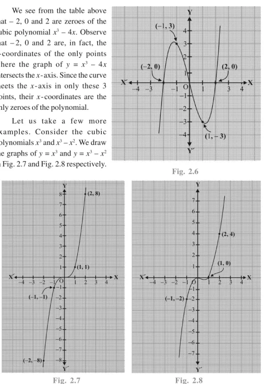
Locating the points of the table on a graph paper and drawing the graph, we see that the graph of y = x3 – 4x actually looks like the one given in Fig. 2.6.
We see from the table above that – 2, 0 and 2 are zeroes of the cubic polynomial x3 – 4x. Observe
that – 2, 0 and 2 are, in fact, the x-coordinates of the only points where the graph of y = x3 – 4x
intersects the x-axis. Since the curve meets the x - axis in only these 3 points, their x - coordinates are the only zeroes of the polynomial.
Let us take a few more examples. Consider the cubic polynomials x3 and x3 – x2. We draw
the graphs of y = x3 and y = x3 – x2
in Fig. 2.7 and Fig. 2.8 respectively.
Fig. 2.7 Fig. 2.8
Note that 0 is the only zero of the polynomial x3. Also, from Fig. 2.7, you can see
that 0 is the x-coordinate of the only point where the graph of y = x3 intersects the
x-axis. Similarly, since x3 – x2 = x2 (x – 1), 0 and 1 are the only zeroes of the polynomial
x3 – x2. Also, from Fig. 2.8, these values are the x - coordinates of the only points
where the graph of y = x3 – x2 intersects the x-axis.
From the examples above, we see that there are at most 3 zeroes for any cubic polynomial. In other words, any polynomial of degree 3 can have at most three zeroes. Remark : In general, given a polynomial p(x) of degree n, the graph of y = p(x) intersects the x-axis at atmost n points. Therefore, a polynomial p(x) of degree n has at most n zeroes.
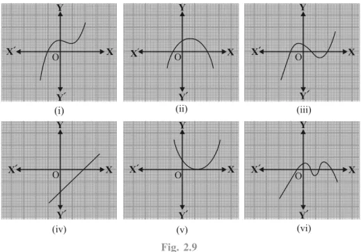
Example 1 : Look at the graphs in Fig. 2.9 given below. Each is the graph of y = p(x), where p(x) is a polynomial. For each of the graphs, find the number of zeroes of p(x).
Fig. 2.9 Solution :
(i) The number of zeroes is 1 as the graph intersects the x-axis at one point only. (ii) The number of zeroes is 2 as the graph intersects the x-axis at two points. (iii) The number of zeroes is 3. (Why?)
(iv) The number of zeroes is 1. (Why?) (v) The number of zeroes is 1. (Why?) (vi) The number of zeroes is 4. (Why?)
EXERCISE 2.1
1. The graphs of y = p(x) are given in Fig. 2.10 below, for some polynomials p(x). Find the
number of zeroes of p(x), in each case.
Fig. 2.10
2.3 Relationship between Zeroes and Coefficients of a Polynomial You have already seen that zero of a linear polynomial ax + b is
b
a
. We will now tryto answer the question raised in Section 2.1 regarding the relationship between zeroes and coefficients of a quadratic polynomial. For this, let us take a quadratic polynomial, say p(x) = 2x2 – 8x + 6. In Class IX, you have learnt how to factorise quadratic
polynomials by splitting the middle term. So, here we need to split the middle term ‘– 8x’ as a sum of two terms, whose product is 6 × 2x2 = 12x2. So, we write
2x2 – 8x + 6 = 2x2 – 6x – 2x + 6 = 2x(x – 3) – 2(x – 3)
So, the value of p(x) = 2x2 – 8x + 6 is zero when x – 1 = 0 or x – 3 = 0, i.e., when
x = 1 or x = 3. So, the zeroes of 2x2 – 8x + 6 are 1 and 3. Observe that :
Sum of its zeroes = 1 3 4 ( 8) (Coefficient of )2 2 Coefficient of
x x
✁ ✂ ✂ ✂
Product of its zeroes = 1 3 3 6 Constant term2 2 Coefficient of x
✄ ✂ ✂ ✂
Let us take one more quadratic polynomial, say, p(x) = 3x2 + 5x – 2. By the
method of splitting the middle term,
3x2 + 5x – 2 = 3x2 + 6x – x – 2 = 3x(x + 2) –1(x + 2)
= (3x – 1)(x + 2)
Hence, the value of 3x2 + 5x – 2 is zero when either 3x – 1 = 0 or x + 2 = 0, i.e.,
when x = 1
3 or x = –2. So, the zeroes of 3x
2 + 5x – 2 are 1
3 and – 2. Observe that :
Sum of its zeroes = 1 ( 2) 5 (Coefficient of )2 3 3 Coefficient of x x ☎ ☎ ✆ ☎ ✝ ✝
Product of its zeroes = 1 ( 2) 2 Constant term2 3 3 Coefficient of x
✄ ✂ ✂
In general, if ✞* and ✟* are the zeroes of the quadratic polynomial p(x) = ax
2 + bx +
c, a ✠ 0, then you know that x – ✞ and x – ✟ are the factors of p(x). Therefore,
ax2 + bx + c = k(x – ✞) (x – ✟), where k is a constant = k[x2 – ( ✞ + ✟)x + ✞✟] = kx2 – k( ✞ + ✟)x + k ✞✟
Comparing the coefficients of x2, x and constant terms on both the sides, we get
a = k, b = – k(✞ + ✟) and c = k✞✟✡ This gives ✞✞ + ✟✟ = –b a , ✞ ✟ ✞ ✟ = c a
* ☛,☞ are Greek letters pronounced as ‘alpha’ and ‘beta’ respectively. We will use later one more letter ‘✌’ pronounced as ‘gamma’.
i.e., sum of zeroes = + ✁ = 2 (Coefficient of ) Coefficient of b x a x ✂ ✂ ✄ , product of zeroes = ✁ = 2 Constant term Coefficient of c a x ☎ .
Let us consider some examples.
Example 2 : Find the zeroes of the quadratic polynomial x2 + 7x + 10, and verify the
relationship between the zeroes and the coefficients. Solution : We have
x2 + 7x + 10 = (x + 2)(x + 5)
So, the value of x2 + 7x + 10 is zero when x + 2 = 0 or x + 5 = 0, i.e., when x = – 2 or
x = –5. Therefore, the zeroes of x2 + 7x + 10 are – 2 and – 5. Now,
sum of zeroes = – 2 (– 5) – (7) (7) – (Coefficient of )2 , 1 Coefficient of
x x
✂
✆ ✄ ✄ ✄
product of zeroes = ( 2) ( 5) 10 10 Constant term2 1 Coefficient of x
✂ ✝ ✂ ✄ ✄ ✄ ✞
Example 3 : Find the zeroes of the polynomial x2 – 3 and verify the relationship
between the zeroes and the coefficients.
Solution : Recall the identity a2 – b2 = (a – b)(a + b). Using it, we can write:
x2 – 3 =
✟x 3✠✟x 3✠
✡ ☛
So, the value of x2 – 3 is zero when x =
3 or x = – 3☞ Therefore, the zeroes of x2 – 3 are
3 and ✌ 3☞ Now, sum of zeroes = 2 (Coefficient of ) , 3 3 0 Coefficient of x x ✂ ✂ ✄ ✄ product of zeroes = ✍ ✎✍ ✎ 2 3 Constant term 3 3 – 3 1 Coefficient of x ✂ ✂ ✄ ✄ ✄ ✞
Example 4 : Find a quadratic polynomial, the sum and product of whose zeroes are – 3 and 2, respectively.
Solution : Let the quadratic polynomial be ax2 + bx + c, and its zeroes be and
✁. We have + ✁ = – 3 = b a ✂ , and ✁ = 2 = c a . If a = 1, then b = 3 and c = 2.
So, one quadratic polynomial which fits the given conditions is x2 + 3x + 2.
You can check that any other quadratic polynomial that fits these conditions will be of the form k(x2 + 3x + 2), where k is real.
Let us now look at cubic polynomials. Do you think a similar relation holds between the zeroes of a cubic polynomial and its coefficients?
Let us consider p(x) = 2x3 – 5x2 – 14x + 8.
You can check that p(x) = 0 for x = 4, – 2, 1 2
✄ Since p(x) can have atmost three zeroes, these are the zeores of 2x3 – 5x2 – 14x + 8. Now,
sum of the zeroes =
2 3 1 5 ( 5) (Coefficient of ) 4 ( 2) 2 2 2 Coefficient of x x ☎ ☎ ☎ ✆ ☎ ✆ ✝ ✝ ✝ ,
product of the zeroes =
3 1 8 – Constant term 4 ( 2) 4 2 2 Coefficient of x ✞ ✟ ✞ ✟ ✠✞ ✠ ✠ .
However, there is one more relationship here. Consider the sum of the products of the zeroes taken two at a time. We have
✡ ☛ 1 1 4 ( 2) ( 2) 4 2 2 ☞ ✌ ☞ ✌ ✟ ✞ ✍ ✞ ✟ ✍ ✟ ✎ ✏ ✎ ✏ ✑ ✒ ✑ ✒ = – 8 1 2 7 14 2 ✂ ✂ ✓ ✔✂ ✔ = 3 Coefficient of Coefficient of x x .
In general, it can be proved that if , ✁, ✕ are the zeroes of the cubic polynomial
+ ✁✁ + ✂✂ = –b a , ✁ + ✁✁ ✂ + ✂ = c a, ✁ ✁ ✂ = – d a . Let us consider an example.
Example 5* : Verify that 3, –1, 1
3
✄ are the zeroes of the cubic polynomial p(x) = 3x3 – 5x2 – 11x – 3, and then verify the relationship between the zeroes and the
coefficients.
Solution : Comparing the given polynomial with ax3 + bx2 + cx + d, we get
a = 3, b = – 5, c = –11, d = – 3. Further p(3) = 3 × 33 –(5 × 32) – (11 × 3) – 3 = 81 – 45 – 33 – 3 = 0, p(–1) = 3 × (–1)3 – 5 × (–1)2 – 11 × (–1) – 3 = –3 – 5 + 11 – 3 = 0, 3 2 1 1 1 1 3 5 11 3 3 3 3 3 p☎ ✆ ☎ ✆ ☎ ✆ ☎ ✆ ✝ ✞ ✟ ✝ ✝ ✟ ✝ ✝ ✟ ✝ ✝ ✠ ✡ ✠ ✡ ✠ ✡ ✠ ✡ ☛ ☞ ☛ ☞ ☛ ☞ ☛ ☞ , = –1 5 11 3 – 2 2 0 9 9 3 3 3 ✄ ✌ ✄ ✍ ✌ ✍ Therefore, 3, –1 and 1 3
✄ are the zeroes of 3x
3 – 5x2 – 11x – 3.
So, we take = 3, ✁ = –1 and ✂ =
1 3 ✄ ✎ Now, 1 1 5 ( 5) 3 ( 1) 2 3 3 3 3 b a ✏✏ ✏ ✑ ✒ ✓✔✕✔✖✗ ✔ ✏ ✔ ✏ ✗ ✏ ✗ ✗ ✗ ✘ ✙ ✚ ✛ , 1 1 1 11 3 ( 1) ( 1) 3 3 1 3 3 3 3 c a ✏ ✑ ✒ ✑ ✒ ✓✕✔✕✖ ✔✖✓✗ ✜ ✏ ✔ ✏ ✜ ✏ ✔ ✏ ✜ ✗✏ ✔ ✏ ✗ ✗ ✘ ✙ ✘ ✙ ✚ ✛ ✚ ✛ , 1 ( 3) 3 ( 1) 1 3 3 d a ✢ ✢ ✢ ✣ ✤ ✥✦✧★ ✩ ✢ ✩ ✢ ★ ★ ★ ✪ ✫ ✬ ✭ .
EXERCISE 2.2
1. Find the zeroes of the following quadratic polynomials and verify the relationship between
the zeroes and the coefficients.
(i) x2 – 2x – 8 (ii) 4s2 – 4s + 1 (iii) 6x2 – 3 – 7x
(iv) 4u2 + 8u (v) t2 – 15 (vi) 3x2 – x – 4
2. Find a quadratic polynomial each with the given numbers as the sum and product of its
zeroes respectively. (i) 1, 1 4 (ii) 1 2 , 3 (iii) 0, 5 (iv) 1, 1 (v) 1 1, 4 4 (vi) 4, 1
2.4 Division Algorithm for Polynomials
You know that a cubic polynomial has at most three zeroes. However, if you are given only one zero, can you find the other two? For this, let us consider the cubic polynomial x3 – 3x2 – x + 3. If we tell you that one of its zeroes is 1, then you know that x – 1 is
a factor of x3 – 3x2 – x + 3. So, you can divide x3 – 3x2 – x + 3 by x – 1, as you have
learnt in Class IX, to get the quotient x2 – 2x – 3.
Next, you could get the factors of x2 – 2x – 3, by splitting the middle term, as
(x + 1)(x – 3). This would give you
x3 – 3x2 – x + 3 = (x – 1)(x2 – 2x – 3)
= (x – 1)(x + 1)(x – 3)
So, all the three zeroes of the cubic polynomial are now known to you as 1, – 1, 3.
Let us discuss the method of dividing one polynomial by another in some detail. Before noting the steps formally, consider an example.
Example 6 : Divide 2x2 + 3x + 1 by x + 2.
Solution : Note that we stop the division process when either the remainder is zero or its degree is less than the degree of the divisor. So, here the quotient is 2x – 1 and the remainder is 3. Also,
(2x – 1)(x + 2) + 3 = 2x2 + 3x – 2 + 3 = 2x2 + 3x + 1
i.e., 2x2 + 3x + 1 = (x + 2)(2x – 1) + 3
Therefore, Dividend = Divisor × Quotient + Remainder
Let us now extend this process to divide a polynomial by a quadratic polynomial.
x + 2 2 + 3 + 1x2 x
2 + 4x2 x
Example 7 : Divide 3x3 + x2 + 2x + 5 by 1 + 2x + x2.
Solution : We first arrange the terms of the dividend and the divisor in the decreasing order of their degrees. Recall that arranging the terms in this order is called writing the polynomials in standard form. In this example, the dividend is already in standard form, and the divisor, in standard form, is x2 +2x + 1.
Step 1 : To obtain the first term of the quotient, divide the highest degree term of the dividend (i.e., 3x3) by the highest degree term of the divisor (i.e., x2). This is 3x. Then
carry out the division process. What remains is – 5x2 – x + 5.
Step 2 : Now, to obtain the second term of the quotient, divide the highest degree term of the new dividend (i.e., –5x2) by the highest degree term of the divisor (i.e., x2). This
gives –5. Again carry out the division process with – 5x2 – x + 5.
Step 3 : What remains is 9x + 10. Now, the degree of 9x + 10 is less than the degree of the divisor x2 + 2x + 1. So, we cannot continue the division any further.
So, the quotient is 3x – 5 and the remainder is 9x + 10. Also,
(x2 + 2x + 1) × (3x – 5) + (9x + 10) = 3x3 + 6x2 + 3x – 5x2 – 10x – 5 + 9x + 10
= 3x3 + x2 + 2x + 5
Here again, we see that
Dividend = Divisor × Quotient + Remainder
What we are applying here is an algorithm which is similar to Euclid’s division algorithm that you studied in Chapter 1.
This says that
If p(x) and g(x) are any two polynomials with g(x) 0, then we can find polynomials q(x) and r(x) such that
p(x) = g(x) × q(x) + r(x), where r(x) = 0 or degree of r(x) < degree of g(x).
This result is known as the Division Algorithm for polynomials. Let us now take some examples to illustrate its use.
Example 8 : Divide 3x2 – x3 – 3x + 5 by x – 1 – x2, and verify the division algorithm. x2 + 2 + 1x 3x – 5 3 + 6x3 x2 +3x – – – –5 – x2 x + 5 –5 – 10x2 x – 5 + + + 9x + 10
Solution : Note that the given polynomials are not in standard form. To carry out division, we first write both the dividend and divisor in decreasing orders of their degrees. So, dividend = –x3 + 3x2 – 3x + 5 and
divisor = –x2 + x – 1.
Division process is shown on the right side.
We stop here since degree (3) = 0 < 2 = degree (–x2 + x – 1).
So, quotient = x – 2, remainder = 3. Now,
Divisor × Quotient + Remainder
= (–x2 + x – 1) (x – 2) + 3
= –x3 + x2 – x + 2x2 – 2x + 2 + 3
= –x3 + 3x2 – 3x + 5
= Dividend In this way, the division algorithm is verified.
Example 9 : Find all the zeroes of 2x4 – 3x3 – 3x2 + 6x – 2, if you know that two of
its zeroes are 2 and 2.
Solution : Since two zeroes are 2 and 2,
✁x 2✂✁x 2✂
✄ ☎ = x
2 – 2 is a
factor of the given polynomial. Now, we divide the given polynomial by x2 – 2.
–x2 + – 1 – + 3x x3 x + 5 x2 – 3 x – 2 2 – 2 + 5x2 x 3 – + x3 x x2 – + – + 2 – 2 + 2x2 x – + – x2 – 2 2x4– 3x3– 3 x –2 x2 + 6 2 – x2 3 + x 1 2 x4 x2 – 3 + x3 + x2 6 – x 2 x2 – 2 – 3 x3 x2 – 2 0 – – 4+ + + 6 x – – +
First term of quotient is
4 2 2 2 2 x x x ✆
Second term of quotient is
3 2 3 3 x x x ✝ ✞✝
Third term of quotient is
2
2 1
x x
So, 2x4 – 3x3 – 3x2 + 6x – 2 = (x2 – 2)(2x2 – 3x + 1).
Now, by splitting –3x, we factorise 2x2 – 3x + 1 as (2x – 1)(x – 1). So, its zeroes
are given by x = 1
2 and x = 1. Therefore, the zeroes of the given polynomial are 1,
2, 2, and 1. 2
EXERCISE 2.3
1. Divide the polynomial p(x) by the polynomial g(x) and find the quotient and remainder
in each of the following :
(i) p(x) = x3 – 3x2 + 5x – 3, g(x) = x2 – 2
(ii) p(x) = x4 – 3x2 + 4x + 5, g(x) = x2 + 1 – x
(iii) p(x) = x4 – 5x + 6, g(x) = 2 – x2
2. Check whether the first polynomial is a factor of the second polynomial by dividing the
second polynomial by the first polynomial: (i) t2 – 3, 2t4 + 3t3 – 2t2 – 9t – 12
(ii) x2 + 3x + 1, 3x4 + 5x3 – 7x2 + 2x + 2
(iii) x3 – 3x + 1, x5 – 4x3 + x2 + 3x + 1
3. Obtain all other zeroes of 3x4 + 6x3 – 2x2 – 10x – 5, if two of its zeroes are 5 and – 5
3 3
✁ 4. On dividing x3 – 3x2 + x + 2 by a polynomial g(x), the quotient and remainder were x – 2
and –2x + 4, respectively. Find g(x).
5. Give examples of polynomials p(x), g(x), q(x) and r(x), which satisfy the division algorithm
and
(i) deg p(x) = deg q(x) (ii) deg q(x) = deg r(x) (iii) deg r(x) = 0
EXERCISE 2.4 (Optional)*
1. Verify that the numbers given alongside of the cubic polynomials below are their zeroes.
Also verify the relationship between the zeroes and the coefficients in each case: (i) 2x3 + x2 – 5x + 2; 1, 1, – 2
2 (ii) x
3 – 4x2 + 5x – 2; 2, 1, 1
2. Find a cubic polynomial with the sum, sum of the product of its zeroes taken two at a
time, and the product of its zeroes as 2, –7, –14 respectively.