HAL Id: hal-00260015
https://hal.archives-ouvertes.fr/hal-00260015v2
Submitted on 5 Mar 2016
HAL is a multi-disciplinary open access
archive for the deposit and dissemination of
sci-entific research documents, whether they are
pub-lished or not. The documents may come from
teaching and research institutions in France or
abroad, or from public or private research centers.
L’archive ouverte pluridisciplinaire HAL, est
destinée au dépôt et à la diffusion de documents
scientifiques de niveau recherche, publiés ou non,
émanant des établissements d’enseignement et de
recherche français ou étrangers, des laboratoires
publics ou privés.
Euler-like modelling of dense granular flows: application
to a rotating drum
Daniel Bonamy, Pierre-Henri Chavanis, Pierre-Philippe Cortet, François
Daviaud, Bérengère Dubrulle, Mathieu Renouf
To cite this version:
Daniel Bonamy, Pierre-Henri Chavanis, Pierre-Philippe Cortet, François Daviaud, Bérengère Dubrulle,
et al.. Euler-like modelling of dense granular flows: application to a rotating drum. European
Physical Journal B: Condensed Matter and Complex Systems, Springer-Verlag, 2009, 68, pp.619.
�10.1140/epjb/2009-00123-6�. �hal-00260015v2�
(will be inserted by the editor)
Euler-like modelling of dense granular flows: application to a
rotating drum
D. Bonamy1, P.-H. Chavanis2, P.-P. Cortet1,3, F. Daviaud3, B. Dubrulle3, and M. Renouf4
1
CEA, IRAMIS, SPCSI, Grp. Complex Systems & Fracture, F-91191 Gif-sur-Yvette, France
2
Laboratoire de Physique Th´eorique, CNRS UMR 5152, Universit´e Paul Sabatier, 118 route de Narbonne, F-31062 Toulouse, France
3
CEA, IRAMIS, SPEC, CNRS URA 2464, Groupe Instabilit´es & Turbulence, F-91191 Gif-sur-Yvette, France
4
Equipe TMI, LaMCoS, CNRS UMR 5259, INSA Lyon, 18-20 rue des sciences, F-69621 Villeurbanne, France
February 28, 2016
Abstract. General conservation equations are derived for 2D dense granular flows from the Euler equation within the Boussinesq approximation. In steady flows, the 2D fields of granular temperature, vorticity and stream function are shown to be encoded in two scalar functions only. We checked such prediction on steady surface flows in a rotating drum simulated through the Non-Smooth Contact Dynamics method. This result is non trivial because granular flows are dissipative and therefore not necessarily compatible with Euler equation. Finally, we briefly discuss some possible ways to predict theoretically these two functions using statistical mechanics.
PACS. 47.57.Gc Granular flow – 47.10.-g General theory in fluid dynamics – 83.80.Fg Granular solids
1 Introduction
The intrinsic dissipative nature of the interactions between the constituent macroscopic particles sets granular media apart from conventional solids, liquids and gases [1]. Un-derstanding the rheology of granular systems is thus rather difficult. Depending on the flow velocity, three regimes are usually distinguished: The rapid flow – gaseous-like – regime where grains interact through binary collisions, is generally described within the framework of the ki-netic theory [2,3,4]; The slow flow – solid-like – regime, where grain inertia is negligible, is most commonly de-scribed using the tools of soil mechanics and plasticity theory [5]. In between these two regimes there exists a dense flow – liquid-like – regime where grain inertia be-comes important but contacts between grains are still rel-evant. This last regime has been widely investigated ex-perimentally, numerically and theoretically (see [6] for a review) in various flow configurations. Several constitu-tive laws have been derived by accounting for non-local effects [7,8,9,10,11], by adapting kinetic theory [12,13,14], by modelling dense flows as partially fluidized flows [15], by considering them as quasi-static flows where the mean motion results from transient fractures modelled as self activated process [16,17,18,19] or more recently by consid-ering them as visco-plastic fluids [20,21,22]. To our knowl-edge, all these approaches fail to account for all the fea-tures experimentally observed.
In some sense, similar difficulties are encountered in the understanding and modelling of turbulent flows. In
that case, the challenge is to relate the Reynolds stresses, based on small scale fluctuations, to large scales or time averaged quantities. A new way to tackle this problem was recently suggested [23,24,25,26], through the consider-ation of non-linear steady solutions of the Euler equconsider-ations, thereby disregarding any non-universal effects induced by (large scale) forcing and (small scale) dissipation. When applied to a turbulent von K´arm´an flow, this approach leads to the characterization of the steady state velocity fields through two scalar functions only, encoding all in-formation about the forcing and the dissipation. In the present paper, this method is generalized to the case of inhomogeneous dense granular flows. As a result, one ob-tains a characterization of the steady state through two scalar functions, dependent on the forcing geometry and on the dissipation processes, that relate the fields of gran-ular temperature, vorticity and stream function. In other words, the knowledge of these two scalar functions is suffi-cient to encode the two-dimensional (2D) hydrodynamical inhomogeneous fields.
The paper is organized as follows: In section 2, the structure of 2D steady granular flows is derived under some specific assumptions. Hydrodynamics and state equa-tions in granular media are briefly discussed in section 2.1. Conservation equations are then rewritten assuming that volume fraction is nearly constant within the flow (Boussinesq approximation) in section 2.2, and then re-stricted to 2D geometries in section 2.3. In section 2.4 the general shape of the stationary solutions is given in the
2 D. Bonamy et al.: Euler-like modelling of dense granular flows: application to a rotating drum
Euler approximation, assuming that, once time-averaged, forcing and dissipation balance locally. In particular, it is shown that these stationary states can be fully charac-terized through the knowledge of two scalar functions F and G. Section 3 confronts these predictions with steady surface flows in rotating drum as obtained in Contact Dy-namics simulations reported in [27] that were shown to re-produce the experimental features observed in references [28,29,30]. The simulation scheme and the description of the simulated systems are briefly recalled in section 3.1. Spatial distribution of the averaged temperature, volume fraction, vorticity and stream function fields are computed within the whole drum, at the grain scale (Sec. 3.2). It appears that these hydrodynamical fields can indeed be described through only two scalar functions F and G. This result is non trivial because it tells us our granu-lar dissipative flow is compatible with non-dissipative Eu-ler equation. The two characteristic functions F and G are then determined from the numerical data (Sec. 3.3), commented (Sec. 3.4) and checked (Sec. 3.5). In the last section of this paper (Sec. 4) some possible ways to predict theoretically these two functions are briefly discussed.
2 Theoretical framework: Conservation
equations within the Boussinesq
approximation
2.1 Granular hydrodynamics
It is commonly assumed that granular media can be de-scribed with continuum models. In all the following, dis-tances, time, velocities and stresses are given in units of d, d/g, √gd and ρ0gd respectively where g refers to the
gravity constant, d to the mean grain diameter, and ρ0to
the mass density of the grains. The mass, momentum and energy conservation equations then lead to:
∂tν + ∇ · (νv) = 0,
∂tνv + (v · ∇) νv = −∇P + νg + Fvisc+ Fforc,
∂tνT + ∇ · (νT v) = −P ∇ · v + Evisc+ Eforc. (1)
In these equations, ν(r, t) is the field of volume frac-tion; v(r, t) is the coarse-grained velocity field given by v(r, t) = hcb(t)ib∈Σ(r) where cb(t) refers to the
instanta-neous velocity of the bead b located at time t within the elementary volume Σ(r) located at position r; g is the gravitational acceleration; T (r, t) is the field of granular temperature defined in term of the RMS part of the ve-locity field, T (r, t) = 1
2h(cb(t)−v(r, t)) 2i
b∈Σ(r); Fforc(r, t),
Eforc(r, t) denote the forcing (apart from gravity force)
ap-plying on this elementary volume and Fvisc(r, t), Evisc(r, t)
stand for the dissipative processes inside this elementary volume. This system has to be supplemented by an equa-tion of state P = g(ν)T and a rheology, i.e. some consti-tutive equations describing Fforc, Eforc, Fvisc, Evisc.
Contrary to classical liquids, the density and temper-ature dependence of transport coefficients play an impor-tant role in determining the flow density. For dilute sys-tems they are usually obtained using kinetic theory of
granular gases [2,3,4] within the Enskog approximation. For dense gases, there is no available systematic theory allowing their description. They are therefore usually pre-scribed using phenomenological models [13] or fitted using experimental [21,22,31] or numerical [32] data. In particu-lar, the equation of state can be written in the high-density limit [21,32]: P ≃ K ν 2 ∗ ν∗− ν T, (2)
where K is a constant and ν∗ the random close packing
limit: ν∗ ≃ 0.82 (resp. ν∗ ≃ 0.64) for 2D (resp. for 3D)
monodisperse packing. At ν = ν∗, this equation therefore
predicts a zero granular temperature, consistent with the absence of motion. As for the dissipative terms and forc-ing, the precise shape of the equation of state shall not be needed in the sequel. This is a distinguished feature of our approach.
2.2 The Boussinesq approximation
For simplicity, one focuses on situations where the vol-ume fraction is nearly constant close to the random close packing limit ν ≈ ν∗. In dense granular flows, this
ap-proximation is generally satisfied within 10 percents [6]. Generalization to non constant volume fraction is possible, but more involved. In that limit, the classical Boussinesq approximation is implemented by neglecting the fluctua-tion of volume fracfluctua-tion in the continuity equafluctua-tion so that it becomes:
∇ · v ≈ 0. (3)
The other conservation equations may then be simplified by defining a reference state with v = 0, T = 0, P = P∗,
ν = ν∗, so that:
∇P∗= ν∗g, (4)
i.e. an hydrostatic equilibrium in the vertical direction. Along with non-zero velocity, we introduce temperature and volume fraction deviations with respect to the refer-ence state as:
ν = ν∗− δν; T = δT ; P = P∗+ δP. (5)
The momentum equation can then be written as: ∂tv+ (v · ∇) v = − 1 ν∇P + g + Fvisc+ Fforc, ≈ −ν1 ∗ ∇δP −δνν2 ∗ ∇P∗+ g − 1 ν∗ ∇P∗ +Fvisc+ Fforc, = −ν1 ∗∇δP − δν ν∗ g+ Fvisc+ Fforc, (6)
where the hydrostatic equilibrium has been used to sim-plify the last equation. A similar treatment of the temper-ature equation leads to:
∂tδT +(v · ∇) δT = Evisc+Eforc−
P∗
ν∗∇·v ≈ E
visc+Eforc.
The system of resulting equations can be further trans-formed so that it involves only temperature fluctuations by using equation (2): δν ν∗ = δT Tref , (8)
where the reference temperature field Tref(r) is given by
Tref = P∗/Kν∗ so that g = K∇Tref, and only the first
order terms in δν/ν∗, δT /Tref and δP/P∗ are kept. The
system of equations of the weakly compressible granular medium then takes the shape:
∇ · v = 0, ∂tv+ (v · ∇) v = − 1 ν∗ ∇δP − δT Tref g+ Fvisc+ Fforc, ∂tδT + (v · ∇) δT = Evisc+ Eforc. (9)
Note that the system can also be formulated in a more classical Boussinesq-like form by introducing the variable θ = δT /Tref and noting that Tref is not a constant (it
varies along the gravity direction), so that: ∇ · v = 0,
∂tv+ (v · ∇) v = −
1 ν∗
∇δP − θg + Fvisc+ Fforc,
∂tθ + (v · ∇) θ + (v · ∇) log Tref= Evisc+ Eforc. (10)
In the sequel, we shall however rather work with the for-mulation (9).
2.3 2D case
We now specialize our granular hydrodynamics to the case of 2D medium, such as flow within a thin rotating drum of diameter 2R, rotated along the y axis at a constant angular velocity Ω as investigated in section 3. If the width of the drum in the y direction is thin with respect to the characteristic length scale of (x, z) motions, the velocity field can be assumed two-dimensional v(x, z, t). In that case, the vorticity is directed along the y axis and the forcing is supplied by the boundary conditions. One can recast equation (9) in cartesian coordinates (x, z) as:
∂xvx+ ∂zvz= 0 , (11) ∂tvx+ vx∂xvx+ vz∂zvx= − 1 ν∗ ∂xδP − gx δT Tref +Fx visc+ Fforcx , ∂tvz+ vx∂xvz+ vz∂zvz= −1 ν∗ ∂zδP − gzδT Tref +Fviscz + Fforcz , ∂tδT + vx∂xδT + vz∂zδT = Evisc+ Eforc , (12)
where x and z indices or superscripts denote the com-ponents of the considered vector in a cartesian referential. Thanks to incompressibility and the 2D nature of the flow,
vxand vzcan be expressed in term of the stream function
ψ defined by:
vx= ∂zψ and vz = −∂xψ .
Calling q the y-component of the vorticity, one gets: q = ∂zvx− ∂xvz= ∆ψ. (13)
where ∆ = ∂2
x+ ∂z2 is the Laplacian. Taking the curl of
the equation for velocity, equations (12) can be recast as: ∂tδT + {ψ, δT } = Evisc+ Eforc, (14)
∂tq + {ψ, q} = K{log Tref, δT } + ∇ × (Fvisc+ Fforc)
where {ψ, φ} = ∂zψ∂xφ − ∂xψ∂zφ is the Jacobian. The
relation between gravity and Trefwas used to simplify the
buoyancy term. This formulation of the stratified Navier-Stokes equation has to be supplemented by appropriate boundary conditions. Notice that only two scalar fields are sufficient to describe the flows under consideration: δT , the granular temperature and q, the y-component of the vorticity.
2.4 Steady state solutions
Let us now consider steady regimes. At the global scale, the dissipation generated by the interactions between grains should balance exactly the external forcing applied by the drum on the packing. From now, we assume that forcing and dissipation equilibrate locally on average. This balance is all the more likely since the considered elementary vol-ume is large. In other words, Fvisc(x, z, t) + Fforc(x, z, t) =
0 and Evisc(x, z, t) + Eforc(x, z, t) = 0, where the overlines
denote averaging over time, and we focus on the left-hand side of equations (14) to see the implications on the form taken by the fields ψ, q and δT . The steady states then obey the averaged equations:
{ψ, δT } = 0 , (15)
{ψ, q} = K{log Tref, δT }.
Neglecting correlations{ψ, δT } ≈ {ψ, δT }, one gets:
{ψ, δT } = 0 , (16)
{ψ, q} = K{log Tref, δT } ,
where the overlines over q, T and ψ are now omitted for sake of simplicity. The first equation is satisfied if
δT = F (ψ), (17)
where F is an arbitrary function. Using the general iden-tity
{f, h(g)} = h′
(g){f, g} = {h′
(g)f, g}, (18) where f , g and h are arbitrary functions, the second equa-tion becomes
{ψ, q + F′
4 D. Bonamy et al.: Euler-like modelling of dense granular flows: application to a rotating drum
Therefore, the general stationary solution of equations (14) is of the form
δT = F (ψ) and q + KF′
(ψ) log Tref= G(ψ), (20)
where F and G are arbitrary functions. Recalling the con-nection between q and ψ, one can fully characterize the stationary states through the two functions F and G as:
δT = F (ψ), ∆ψ = q = −K F′
(ψ) log Tref+ G(ψ). (21)
It should be emphasized that the functions F and G de-pend on the forcing and dissipation. Indeed, the compe-tition between these two effects are responsible for the selection of the precise shape for F and G. But once these functions are known, one can solve the second equation of (21) to get ψ as a function of x and z, and then derive from this expression the temperature and velocity profile. To close the system of conservation equations, it is then sufficient to give the expression for F and G. There are probably several ways to prescribe these functions. For ex-ample, one could use a statistical mechanics approach in order to select their “most probable” form depending on macroscopic constraints and microscopic processes, using methods of information theory (see e.g. [23,24,33,34] for illustrations in turbulence). One could also follow the pro-cedure used in rheology studies, and try to define these functions through “minimal” experimental or numerical measurements performed on the considered system.
3 Application to simulated steady surface
flows
The formalism described in the previous section is now ap-plied to the inhomogeneous steady surface flows observed in rotating drums.
3.1 Simulation methodology
The simulations have been performed using Non-Smooth Contact Dynamics approach [35,36]. The algorithms bene-fit from parallel versions [37,38] which show their efficiency in the simulation of large systems. The scheme has been described in detail elsewhere [27] and is briefly recalled below: An immobile drum of diameter D0= 45 cm is
half-filled with 7183 rigid disks of density ρ0= 2.7 g.cm−3and
diameter uniformly distributed between 3 and 3.6 mm. The weak polydispersity introduced in the packing pre-vents 2D ordering effects. The normal restitution coeffi-cient between two disks (resp. between disks and drum) is set to 0.46 (resp. 0.46) and the friction coefficient to 0.4 (resp. 0.95). Once the packing is stabilized, a constant rotation speed ranging from 2 to 15 rpm is imposed to the drum. After one round, a steady continuous surface flow is reached. One starts then to capture 400 snapshots equally distributed over one rotation of the drum.
0.43 m/s
0 m/s
2.5
0
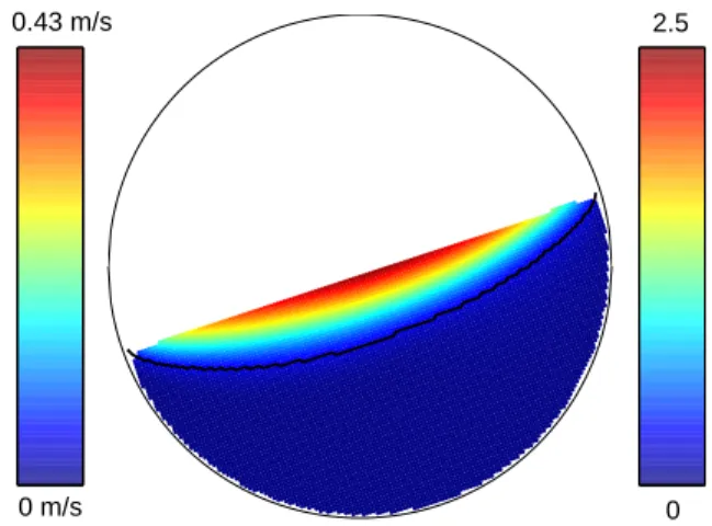
Fig. 1. x-component of the time and ensemble averaged ve-locity field in the simulated 2D rotating drum for a Ω = 6 rpm rotation speed. The black line shows the interface between the flowing layer and the “static” packing. Velocities are expressed in m.s−1 (left-hand colorbar) or non-dimensionalized by √gd
(right-hand colorbar) where g refers to the gravity constant and d to the mean diameter of the beads (see text for details).
For each bead of each of the 400 frames within a given numerical experiment, one records the position r of its center of mass and its “instantaneous” velocity c aver-aged over the time step δt = 6 × 10⁻³ s of the simulation.
For each rotation velocity, we have performed 20 experi-ments starting from different initial packing of the beads. The reference frame ℜ is defined as the frame rotating with the drum that co¨ıncides with the reference frame ℜ0= (ex, ez) fixed in the laboratory so that ex(resp. ez)
is parallel (resp. perpendicular) to the free surface (Fig. 1). The drum is then divided into elementary square cells Σ(x, z) of size set equal to the mean bead diameter.
The average value of a field a(x, z, t) at a position (x, z) is computed as a mixture of time and ensemble average. Indeed, we performed averages of a quantity defined at the grain scale over all the beads in all the 400 frames of all the 20 experiments whose center of mass is within the cell located at (x, z). Figure 1 shows the spatial distribution of the x-component of the time-averaged velocity field v(x, z) as obtained within this procedure. The flowing layer and the static phase are then defined as the point where vx
is above and below a threshold value arbitrary chosen to 0.2. Let us note that all the results presented below do not depend on this threshold value. The interface between the two phases as defined within this procedure is represented as a black line in figure 1.
3.2 Spatial distribution of the relevant continuous fields within the drum
Let us first determine the granular temperature field within the drum. Calling ci(t) the instantaneous velocity of a
bead i at a given time t, the fluctuating part of the ve-locity δci(t) is defined as δci(t) = ci(t) − v(x, z) where
0.003 m2.s−2 0 m2.s−2 0.1 0
(a)
0.003 m2.s−2 0 m2.s−2 0.1 0(b)
0.9 0.7(c)
0.84 0.78(d)
26 s−1 −26 s−1 0.5 −0.5(e)
11 s −1 0 s−1 0.2 0(f)
Fig. 2. Spatial distribution of various continuous fields measured within the drum for experiments with a Ω = 6 rpm rotation speed. Left: Typical snapshot of the instantaneous spatial distribution of granular temperature (a), volume fraction (c) and vorticity (e) within the rotating drum. Right: Time and ensemble averaged field of temperature (b), volume fraction (d) and vorticity (f). The average was taken over the 400 snapshots of each of the 20 experiments for Ω = 6 rpm. Temperatures are expressed in m2
.s−2 (left-hand colorbar) or non-dimensionalized by gd (right-hand colorbar). Vorticities are expressed in s−1
(left-hand colorbar) or non-dimensionalized bypg/d (right-hand colorbar) where g refers to the gravity constant and d to the mean diameter of the beads (see text for details).
contains the bead i. One can then associate a granular temperature Ti(t) = 12δc2i(t) to the considered bead.
Fig-ure 2a shows a typical snapshot of the instantaneous tem-perature distribution within the drum as obtained using this procedure. Two phases can be clearly distinguished. Within the static phase, the temperature is very close to zero. Within the flowing layer, the spatial distribution of instantaneous local temperature shows large fluctuations, with hot and cold spots gathered in transient clusters of various sizes. This structure of hot and cold aggregates
probably has its origin in the existence of “jammed” ag-gregates embedded in the flow, as evidenced in rotating drum experiments [39]. Since we are primarily interested in steady averaged fields in relation with the theoretical framework developed in section 2, we focus on the spatial distribution of the temperature after averaging over the 400 snapshots of each of the 20 experiments performed for a given rotation velocity. The corresponding – time and ensemble – averaged temperature field is represented in figure 2b.
6 D. Bonamy et al.: Euler-like modelling of dense granular flows: application to a rotating drum
Vorono¨ı tessellation is then used to associate an in-stantaneous elementary volume as defined in Continuum Mechanics to each bead i on each snapshot (see e.g. [27] for related discussion). Calling Ai the area of the Vorono¨ı
polyhedra enclosing the grain i, the instantaneous volume fraction νi is defined as νi = πd2i/4Ai where di denotes
the diameter of bead i. Typical snapshot of the result-ing instantaneous map of volume fraction is presented in figure 2c. Apart from a very narrow region – about one bead diameter wide – at the free surface and along the drum boundary, the volume fraction appears almost con-stant, around 0.825, with apparent random fluctuations with standard deviation around 0.04. However, the – time and ensemble – averaged field of volume fraction presented in figure 2d reveals that ν(x, z) decreases slightly within the flowing layer, as expected since dilatancy effects should accompany granular deformation [40].
To compute the instantaneous vorticity ωi associated
to each bead i of each snapshot, the following procedure is adopted: (i) The Vorono¨ıpolygon associated with the bead i is dilated homothetically by a factor two, so that each edge goes through one of the neighboring beads’center; (ii) the circulation Γi(t) =Pjcj(t).sj(t) is calculated around
the resulting polygon – each point of a given segment sjis
assumed to have a constant velocity cj(t) equal to the one
of the embedded bead; (iii) the instantaneous vorticity ωi(t) is then defined as qi(t) = Γi(t)/Ai(t) where Ai(t)
refers to the area of the initial Vorono¨ı polygon.
A typical snapshot of the instantaneous vorticity dis-tribution within the drum as obtained using this proce-dure is presented in figure 2e. This distribution is complex. It exhibits large fluctuations that self-organize into tran-sient network of 1D chains. The characterization of this transient structure is postponed to future work. Figure 2f presents the – time and ensemble – averaged vorticity field in the drum for Ω = 6 rpm.
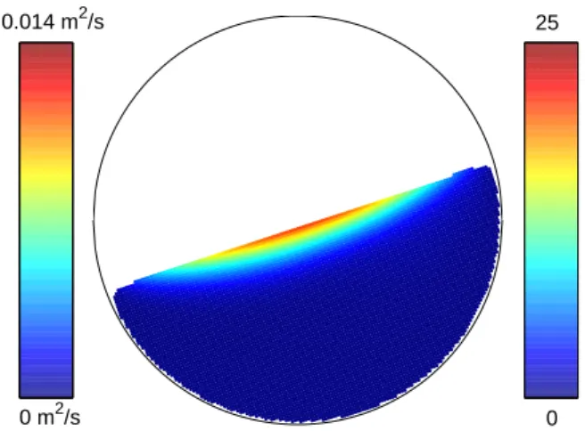
The last continuous field of interest in relation with the theoretical framework presented in section 2 is the stream function ψ(x, z). Its value is set to ψ = 0 at the drum boundary. The value ψ(x, z) is then defined as the flow rate going through a line connecting the point M at position r(x, z) to any point at the drum boundary like e.g.point M0 at position r0(x, −pD02/4 − x2):
ψ(x, z) = Z z −√D2 0/4−x 2 vx(x, u)du (22)
The resulting spatial distribution of the stream func-tion is shown in figure 3.
3.3 Determination of the two scalar functions within Boussinesq approximation
Let us first determine the value of the parameters K and ν∗involved in the equation of state given by equation (2).
This determination requires the pressure field P∗ in the
reference frame, when v = 0. From equation (4), one gets
0.014 m2/s
0 m2/s
25
0
Fig. 3.Spatial distribution of the time and ensemble averaged stream function ψ in the drum for Ω = 6 rpm. The stream function is expressed in m2
.s−1 (left-hand colorbar) or
non-dimensionalized by d√gd (right-hand colorbar) where g refers to the gravity constant and d to the mean diameter of the beads (see text for details).
0 0.01 0.02 0.03 0.04 0.78 0.79 0.8 0.81 0.82 0.83
ν
(x
,z
)
−T (x, z)/z cos θ
Fig. 4.Time and ensemble averaged volume fraction ν(x, z) as a function of the ratio T (x, z)/z cos θ for Ω = 6 rpm. For this rotation speed, the mean slope of the free surface was measured to be θ ≃ 19.7◦[27]. The straight line is a fit given by equation
(23) with K ≃ 1.1 and ν∗ ≃ 0.822. The temperature is
non-dimensionalized by gd where g refers to the gravity constant and d to the mean diameter of the beads (see text for details).
P∗(x, z) = −zν∗cos θ where θ is the slope of the free
sur-face. Equation (8) can then be rewritten as:
ν(x, z) = ν∗+ Kν∗
T (x, z)
z cos θ (23) The time and ensemble averaged local volume fraction ν(x, z) is plotted as a function of the ratio T (x, z)/z cos θ in figure 4. The values of both ν∗ and K can then be
deduced. The volume fraction ν∗ is found to be ν∗ ≃
0.824 ± 0.003 independently of the rotation velocity. The parameter K is found to be close to unity, weakly
depen-dent on the rotating speed Ω1(see Tab. 1). The reference
temperature field Tref(x, z) = −z cos θ/K is then known.
Ω 2 rpm 4 rpm 5 rpm 6 rpm 10 rpm 15 rpm K 0.4 0.8 1.1 1.1 1 0.8 Table 1. Variation of the parameter K involved in the state equation (2) with respect to the rotating velocity Ω of the drum. K ≃ 1 is found weakly dependent on the rotating veloc-ity Ω.
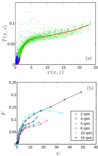
The knowledge of both the field T (x, z) and ψ(x, z) allows to check the first equation in system (21). Figure 5a shows T (x, z) as a function of ψ(x, z) for Ω = 6 rpm. The data points clearly gather along a single function. It is worth to emphasize that such result would have been trivial in unidirectional “homogeneous” flows such as ob-served in plane shear or inclined plane geometry: in such flows, all the continuum quantities depend on a single spa-tial coordinate and are thus naturally related univocally by single functions. On the contrary, the fact that the 2D fields T (x, z) and ψ(x, z) can be related by a single func-tion in the inhomogeneous multidirecfunc-tional surface flow considered here, where the continuum quantities depend on both spatial coordinates x and z, is highly non trivial and constitutes then a rather severe test for the approach derived in section 2. The function F (red line in Fig. 5a) is defined by averaging the values T falling into logarith-mically distributed bins defined along ψ. The functions F obtained using this procedure for the various rotating speeds Ω are represented in figure 5b.
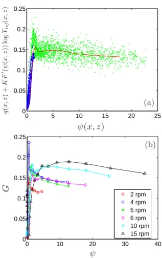
One can now determine the second closure relation G(ψ). The function F (ψ) defined in the previous section (red line in Fig. 5a) is first derived numerically. The re-sulting function is then applied at each point (x, z) to the field ψ(x, z). Since the reference temperature Tref(x, z) =
−z cos θ/K and the vorticity field q(x, z) are also known at each point, one can deduce the value of the field q(x, z) + KF′(ψ(x, z)) log T
ref(x, z) at each point, and plot it as a
function of ψ(x, z) (see Fig. 6a). Again, the points clearly gather along a single curve. The function G (red line in figure 6a) is then defined by averaging the values q(x, z) + KF′(ψ(x, z)) log T
ref(x, z) falling into logarithmically
dis-tributed bins defined along ψ. The functions G obtained using this procedure for the various rotating speeds Ω are represented in figure 6b.
3.4 Discussion of the results
Our determination of the two scalar functions calls for some comments. A first noticeable feature is that the func-tion extends smoothly, without any noticeable transifunc-tion,
1
Strictly speaking, the parameter K is found to be signif-icantly smaller for Ω = 2 rpm. However, for this particular rotating speed the flowing layer is very thin. As a result, the variation range of both ν(x, z) and T (x, z) is very small and makes the fit with equation (23) rather imprecise.
0 5 10 15 20 25 0 0.05 0.1
(a)
ψ(x, z)
T
(x
,z
)
0 10 20 30 40 50 60 0 0.05 0.1 0.15 0.2 0.25 2 rpm 4 rpm 5 rpm 6 rpm 10 rpm 15 rpm(b)
ψ
F
Fig. 5. (a) Variation of the local temperature T (x, z) as a function of the local stream function ψ(x, z) for Ω = 6 rpm. Each dot of the cloud corresponds to an elementary square cell Σ(x, z) of size equal to the mean bead diameter. Green/light gray dots (resp. blue/strong gray dots) correspond to points that belong to the flowing layer (resp. to the static phase). The red line shows the function hT i = F (ψ) where hT i is de-fined as the average of the values T for the cells Σ(x, z) whose ψ(x, z) fall into logaritmically distributed bins. (b) Variation of F (ψ) as a function of Ω. The temperature and stream function are non-dimensionalized by gd and d√gd respectively, where g refers to the gravity constant and d to the mean diameter of the beads (see text for details).
from the static to the flowing region. This is quite remark-able, since both phases are characterized by different dy-namical properties, and since our hydrodynamic descrip-tion presumably applies best within the flowing region. The main difference between the two phases is in the scat-tering of the data along the fit: It is larger in the flowing region than in the static region. This may be traced to correlated fluctuations that have been neglected in our approach (see after Eq. (15)) and that are larger in the flowing region. It would be interesting to see if a larger statistics leads to a reduction of this scattering.
An interesting comparison can also be made with re-spect to a real fluid system, where a similar approach can be used and where dissipation is made through ordinary viscosity. In that case, it has been shown in [25] that the
8 D. Bonamy et al.: Euler-like modelling of dense granular flows: application to a rotating drum 0 5 10 15 20 25 0 0.05 0.1 0.15 0.2 0.25
(a)
ψ(x, z)
q( x ,z ) + K F ′ (ψ (x ,z )) lo g Tre f (x ,z ) 0 10 20 30 40 0 0.05 0.1 0.15 0.2 0.25 2 rpm 4 rpm 5 rpm 6 rpm 10 rpm 15 rpm(b)
ψ
G
Fig. 6. (a) Variation of the local field q(x, z) + KF′(ψ(x, z)) log T
ref(x, z) as a function of the local stream
function ψ(x, z) for Ω = 6 rpm. Each dot of the cloud corre-sponds to an elementary square cell Σ(x, z) of size equal to the mean bead diameter. Green/light gray dots (resp. blue/strong gray dots) correspond to points that belong to the flowing layer (resp. to the static phase). The red line shows the function hq+KF′(ψ) log T
refi = G(ψ) where h i is defined as the average
on the cells Σ(x, z) with values ψ(x, z) which fall into logar-itmically distributed bins. (b) Variation of G(ψ) as a function of Ω. The temperature, vorticity and stream function are non-dimensionalized by gd,pg/d and d√gd respectively, where g refers to the gravity constant and d to the mean diameter of the beads (see text for details).
determination of the scalar function is valid only in the bulk flow region. Outside this region, the data scatters randomly, without forming any specific shape. A possible explanation was that outside the bulk, i.e. closer to the boundaries and the flow forcing devices, viscous and forc-ing processes become important and do not balance locally on average as assumed here. The reason why it works so well in the granular case, without any need of selecting any flow region, may lie in the local character of the dissi-pative processes that precludes any long-range correlation between forcing and dissipation.
3.5 Consistency check
As a consistency check, we can use the experimental curve F and G to recompute the velocity and temperature fields and check that they agree with profiles obtained in a ro-tating drum. From figures 5 and 6, one sees that, in that phase, F is asymptotically linear F ∼ aψ, while G is ap-proximately constant, G ∼ b. Inserting these shapes in equation (21) leads to:
δT = aψ,
∆ψ = −aK log(−z cos θ/K) + b (24) Integrating the second equation with respect to z, one finds: ψ = (b − aK log(cos θ/K))z 2 2 + 3 2aKz − aK 2 z 2 log(−z) (25) so that the temperature profile is quadratic, with logarith-mic correction and the velocity profile is linear, with log-arithmic correction. This is indeed the behavior observed in our rotating drum and, more generally, in this type of flow in the flowing phase [6,11,27,29].
In the static phase, F appears quadratic in ψ, F ∼ cψ2
and G is linear G ∼ dψ. Therefore, equation (21) becomes: δT = cψ2,
∆ψ = (d − 2cK log Tref)ψ (26)
The solution for ψ is in this case ψ = ψ0exp(h(z)),
h′2(z) + h′′
(z) = d − 2cK log Tref> 0, (27)
so that both the velocity profile and the temperature pro-files are exponential, with algebraic corrections. This is indeed the behavior observed in the static phase of our rotating drum or other similar type of flows [29,41,42,43].
4 Concluding discussion
In this paper, we investigate the steady states in 2D dense granular flows within the Boussinesq-Euler approxima-tion, assuming local balance between time-averaged forc-ing and dissipation exerted on an elementary volume. We derived specific relations between the continuum fields (temperature, vorticity and stream function). In partic-ular, we show that the fully 2D steady states can be com-pletely encoded in two scalar functions F and G. This prediction is then successfully checked onto the stationary states of a dense inhomogeneous multidirectional granu-lar flow in a rotating drum. This means that stationary states of the rotating drum can be described by a pure Euler description, where neither the forcing, nor the dissi-pation are explicitly taken into account. In the strict Euler equation framework, both F and G would supposedly be determined by boundary and initial conditions. However, in our approach, these conditions are only effective and
the functions F and G account implicitly for the dissipa-tion processes and the forcing geometry of the considered forced dissipative flow. In this sense, the two scalar func-tions F and G can be seen as fully encoding the 2D fields for temperature and velocity in our apparatus. This rep-resents a reduction of the complexity of the description of the rotating drum granular flows.
The main question in the present framework is there-fore now to understand and predict the shape of F and G as a function of the forcing and dissipation. From an experimental or numerical point of view, one may try and find empirical laws from variation of the control parame-ters like rotation speed, size of the beads, friction coeffi-cient, etc. From a theoretical point of view, it would be very interesting to be able to derive these functions from a systematic theory. In a forthcoming paper, we explore a strategy, based upon the statistical mechanics. This will lead to a selection of the possible shapes of F and G based on conservation laws and maximisation of an information entropy. Moreover, this strategy leads to Gibbs distribu-tions providing a direct link between the function F and G and the fluctuations of physical quantities. Therefore, from the knowledge of the mean flow, one will be able to predict the velocity fluctuations. In this respect, the present approach provides a useful insight for dense gran-ular flow in rotating drum and could be applied to other granular flows. Finally, we stress that the present approach relies heavily on the 2D character of the flow, that allows the description of the flow non-linearities in terms of Jaco-bian. This feature can be easily generalized to the case of 3D flows with symmetries [24]. Its extension to arbitrary 3D geometry is currently the subject of a very active re-search.
We gratefully acknowledge O. Dauchot for a critical reading of the manuscript. Simulations are performed us-ing LMGC90 software. This work is supported by the CINE (Centre d’Information National et d’Enseignement) under the project lmc2644. We are grateful to S. Aumaˆıtre, O. Dauchot, F. Leschenault and R. Monchaux for many enlightening discussions.
References
1. H.M. Jaeger, S.R. Nagel, R.P. Behringer, Rev. Mod. Phys. 68(4), 1259 (1996)
2. S.B. Savage, D.J. Jeffrey, J. Fluid Mech. 110, 255 (1981) 3. J.T. Jenkins, S.B. Savage, J. Fluid Mech. 130, 187 (1983) 4. C.K.K. Lun, S.B. Savage, Acta Mech. 63, 15 (1986) 5. R.M. Nedderman, Statics and Kinematics of Granular
Ma-terials (Cambridge University Press, Cambridge, 1992) 6. G.D.R. Midi, Eur. Phys. J. E 14, 341 (2004)
7. P. Mills, D. Loggia, M. Texier, Europhys. Lett. 45, 733 (1999)
8. B. Andreotti, S. Douady, Phys. Rev. E 63, 031305 (2001) 9. J.T. Jenkins, D.M. Hanes, Phys. Fluids 14, 1228 (2002) 10. D. Bonamy, P. Mills, Europhys. Lett. 63, 42 (2003) 11. J. Rajchenbach, Phys. Rev. Lett 90, 144302 (2003) 12. S.B. Savage, J. Fluid Mech. 377, 1 (1998)
13. L. Bocquet, W. Losert, D. Schalk, T.C. Lubensky, J.P. Gollub, Phys. Rev. E 65(1), 01307 (2002)
14. L.S. Mohan, K.K. Rao, P.R. Nott, J. Fluid Mech 457, 377 (2002)
15. I.S. Aranson, L.S. Tsimring, Phys. Rev. E 65 061303 (2002)
16. O. Pouliquen, R. Gutfraind, Phys. Rev. E 53(1), 552 (1996)
17. G. Debregeas, C. Josserand, Europhys. Lett. 52, 137 (2000)
18. O. Pouliquen, Y. Forterre, S.L. Dizes, Adv. complex Sys-tem 4, 441 (2001)
19. A. Lemaitre, Phys. Rev. Lett. 89, 064303 (2002)
20. I. Iordanoff, M.M. Khonsari, ASME J. Tribol. 14, 341 (2004)
21. F. Da Cruz, S. Eman, M. Prochnow, J.-N. Roux, F. Chevoir, Phys. Rev. E 72, 021309 (2005)
22. P. Jop, Y. Forterre, O. Pouliquen, Nature 441, 727 (2006) 23. N. Leprovost, B. Dubrulle, P.-H. Chavanis, Phys. Rev. E
71, 036311 (2005)
24. N. Leprovost, B. Dubrulle, P.-H. Chavanis, Phys. Rev. E 73, 046308 (2006)
25. R. Monchaux, F. Ravelet, B. Dubrulle, A. Chiffaudel, F. Daviaud, Phys. Rev. Lett. 96, 124502 (2006)
26. R. Monchaux, P.-P. Cortet, P.-H. Chavanis, A. Chiffaudel, F. Daviaud, P. Diribarne, B. Dubrulle, Phys. Rev. Lett. 101, 174502 (2008)
27. M. Renouf, D. Bonamy, F. Dubois, P. Alart, Phys. Fluids 17(10), 103303 (2005)
28. J. Rajchenbach, Adv. Phys. 49, 229 (2000)
29. D. Bonamy, F. Daviaud, L. Laurent, Phys. Fluids 14(5), 1666 (2002)
30. D. Bonamy, F. Daviaud, L. Laurent, P. Mills, Gran. Matt. 4, 183 (2003)
31. P. Jop, Y. Forterre, O. Pouliquen, J. Fluid Mech. 541, 167 (1990)
32. R.J. Speedy, J. Chem. Phys. 110, 4559 (1999)
33. P.-H. Chavanis, J. Sommeria, Phys Rev. Lett. 78, 3302 (1997)
34. P.-H. Chavanis, J. Sommeria, Phys Rev. E 65, 026302 (2002)
35. J.-J. Moreau, in Non Smooth Mechanics and Applica-tions, CISM Courses and Lectures, edited by P.-D. Pana-giotopoulos (Springer-Verlag, Wien, New York, 1988), p. 1
36. M. Jean, Comp. Meth. Appl. Mech. Engrg. 177, 235 (1999) 37. M. Renouf, P. Alart, Comp. Meth. Appl. Mech. Engrg.
194, 2019 (2004)
38. M. Renouf, F. Dubois, P. Alart, J. Comput. Appl. Math. 168, 375 (2004)
39. D. Bonamy, F. Daviaud, L. Laurent, M. Bonetti, J.-P. Bouchaud, Phys. Rev. Lett. 89, 034301 (2002)
40. O. Reynolds, Phyl. Mag. Ser. 5 20, 469 (1885)
41. T.S. Komatsu, S. Inagasaki, N. Nakagawa, S. Nasuno, Phys. Rev. Lett. 86, 1757 (2001)
42. S. Courrech du Pont, R. Fisher, P. Gondret, B. Perrin, M. Rabaud, Phys. Rev. Lett. 94, 048003 (2005)
43. J. Crassous, J.-F. Metayer, P. Richard, C. Laroche, J. Stat. Mech., P03009 (2008).