HAL Id: hal-01855264
https://hal.inria.fr/hal-01855264
Submitted on 7 Aug 2018
HAL is a multi-disciplinary open access
archive for the deposit and dissemination of
sci-entific research documents, whether they are
pub-lished or not. The documents may come from
teaching and research institutions in France or
abroad, or from public or private research centers.
L’archive ouverte pluridisciplinaire HAL, est
destinée au dépôt et à la diffusion de documents
scientifiques de niveau recherche, publiés ou non,
émanant des établissements d’enseignement et de
recherche français ou étrangers, des laboratoires
publics ou privés.
A Methodology for Performance Benchmarking of
Mobile Networks for Internet Video Streaming
Muhammad Khokhar, Thierry Spetebroot, Chadi Barakat
To cite this version:
Muhammad Khokhar, Thierry Spetebroot, Chadi Barakat. A Methodology for Performance
Bench-marking of Mobile Networks for Internet Video Streaming. MSWIM 2018 - The 21st ACM
Interna-tional Conference on Modeling, Analysis and Simulation of Wireless and Mobile Systems, Oct 2018,
Montreal, Canada. �10.1145/3242102.3242128�. �hal-01855264�
A Methodology for Performance Benchmarking of Mobile
Networks for Internet Video Streaming
Muhammad Jawad Khokhar, Thierry Spetebroot, Chadi Barakat
Université Côte d’Azur, Inria, France
[email protected], [email protected], [email protected]
ABSTRACT
Video streaming is a dominant contributor to the global Internet traffic. Consequently, gauging network performance w.r.t. the video Quality of Experience (QoE) is of paramount importance to both telecom operators and regulators. Modern video streaming systems, e.g. YouTube, have huge catalogs of billions of different videos that vary significantly in content type. Owing to this difference, the QoE of different videos as perceived by end users can vary for the same network Quality of Service (QoS). In this paper, we present a methodology for benchmarking performance of mobile operators w.r.t Internet video that considers this variation in QoE. We take a data-driven approach to build a predictive model using supervised machine learning (ML) that takes into account a wide range of videos and network conditions. To that end, we first build and analyze a large catalog of YouTube videos. We then propose and demonstrate a framework of controlled experimentation based on active learning to build the training data for the targeted ML model. Using this model, we then devise YouScore, an estimate of the percentage of YouTube videos that may play out smoothly under a given network condition. Finally, to demonstrate the benchmarking utility of YouScore, we apply it on an open dataset of real user mobile network measurements to compare performance of mobile operators for video streaming.
KEYWORDS
Quality of Experience; Active Learning; Internet Video; Controlled Experimentation; Mobile Network Measurements
1
INTRODUCTION
Network operators constantly strive to provide the best Quality of Experience (QoE) to their end users to ensure business growth. As video streaming is the dominant contributor to the global Inter-net traffic of today, analyzing mobile Inter-network performance w.r.t video QoE has become extremely important from both a telecom operator and a regulator point of view. Modern video streaming systems e.g., YouTube, DailyMotion, store their video contents in several resolutions giving the user the choice to either manually select the resolution of playout or rely on client player to automat-ically switch between video resolutions according to underlying network performance using adaptive bitrate streaming technol-ogy (DASH). The literature on Internet Video suggests that QoE of video streaming can be modeled using application level Quality of Service (QoS) features such as the initial join time, number and duration of stalling/re-buffering events, bitrate switches and resolu-tion of individual chunks played out [1], [2], [3]. Recent works have
This work is supported by the French National Research Agency under grant BottleNet no. ANR-15-CE25-0013 and Inria Project Lab BetterNet.
shown that network level Quality of Service (QoS) measurements (e.g., bandwidth, delay, loss rate) can be used to estimate applica-tion QoS features that can be in their turn used to gauge QoE of Internet video [2]. This is because the network QoS has a direct impact on the application level QoS, and then on the QoE. This has also motivated the use of Machine Learning (ML) to directly link the network QoS to the application QoE resulting in what are called QoS-QoE estimation models (e.g. [4]). Such models can be applied on large datasets of network level measurements provided by crowd-sourcing apps such as RTR-NetTest [5] and MobiPerf [6] to estimate video QoE of end users in today’s mobile networks.
Today’s content providers typically have billions of videos that vary significantly in content from fast motion sports videos to static video lectures. Building a model that represents all such contents is a challenge. Prior works on modeling video QoE either take a very small subset of videos [7], [8], or use datasets generated inside the core networks without elaborating on the kind of videos played out [2]. Such works miss out to highlight the variation in the QoE of videos due to the difference in contents and the span of network QoS. In this paper, we propose to quantify this QoE variation and answer the following questions: for a catalog of given video content provider, how much would the QoE of videos of a given resolution (manually set by the end user) differ under the same network conditions? Differently speaking, what percentage of videos of a certain resolution play out smoothly under a given network QoS? Such questions are pertinent in today’s 3G/4G mobile networks where capacity or coverage related issues can lower the bandwidth and inflate the delay and the loss rate of packets . Hence, it is important for operators to accurately gauge the extent to which the QoE of video streaming portals, e.g. YouTube, can degrade in congested/bad coverage scenarios considering the diversity and popularity in the contents offered by today’s Internet.
The Internet videos can vary significantly from high motion sports/music videos to static videos with very little motion. This difference in contents may be quantified by using some complex image/video processing techniques, however, in our work we resort to use a much simpler metric of average video encoding bitrate to quantify the difference. It is calculated by dividing the total video size (in bytes or bits) by the duration of the video (in seconds). Since videos are compressed using video codecs such as H.264 which try to minimize the bitrate while not impacting the visual quality, the type of content affects the encoded bitrate of the video. For example, a high motion video is supposed to have a higher bitrate compared to a slow motion video for the same resolution. The video bitrate in turn affects the network QoS required for smooth play out. For example, for a high bitrate video, more bandwidth is required to ensure acceptable smooth play out compared to videos of lower bitrate for the same resolution.
Based on this basic relationship between video bitrate, QoS and QoE, we propose a methodology to devise global QoE indicators for Internet video content provider systems that would give estimates into the percentage of videos (in the targeted catalog) that may play out smoothly under a given network QoS. This QoE indicator which we call YouScore allows to gauge network performance considering the intrinsic variability in the contents of the catalog of the target content provider. We consider YouTube in our work as it is the most widely used video streaming service of today’ Internet. To devise YouScore, we first collect a large catalog of YouTube videos that contains video bitrate and other meta-data information about the videos. We then build a training QoS-QoE dataset by playing out a diverse set of YouTube videos (sampled from the catalog) under a wide range of network conditions; the sampling of the videos and the selection of the relevant conditions for network emulation is done using active learning, an efficient sampling methodology that we developed in a prior work for the YouTube experimen-tation case with network QoS only [4]; in this paper, we extend our prior work to sample the content space (video bitrate) as well. The collected dataset is used to train supervised ML algorithms to build the predictive model that takes as input the video bitrate and network QoS to estimate the QoE. Using this ML model, we devise YouScore which quantifies the variation in video QoE for a case of YouTube. Finally, we demonstrate a performance analysis for different mobile operators by applying YouScore on a dataset of real user measurements obtained in the wild. Overall, we present a methodology for benchmarking mobile networks’ performance w.r.t to Internet video streaming. Our approach is general and can be used to devise global QoE scores for any video content provider. Rest of the paper is organized as follows: in Sec. 2, we discuss our methodology for building the YouTube video catalog and present its statistical analysis. In Sec. 3, we discuss our framework for building the QoS-QoE dataset. We devise YouScore in Sec. 4 and apply it on the dataset of real network access measurements and demonstrate a comparative analysis between mobile operators in Sec. 5. We discuss related work in Sec. 6 and conclude the paper in Sec. 8.
2
THE VIDEO CATALOG
2.1
Methodology
To get a large and representative corpus of YouTube video catalog, we use the YouTube data API and search YouTube with specific keywords obtained from Google Top Trends website. Specifically, we use around 4k keywords extracted from the top charts for each month from early 2015 to November 2017. We had to increase the number of keywords as the YouTube API restricts the number of videos returned for each keyword dynamically in the range of few hundreds. The search criterion was set to fetch short high definition (HD) videos (less than 4 minutes) for the region of USA. To obtain the bitrate information, we rely on Google’s get_video_info API that returns the video meta-data for each video identifier. Overall and after some processing, we build a dataset of around 12 million entries for 1.2 Million unique video identifiers. Each entry in this dataset represents a unique video identified by a video ID and its available resolution (identified by an itag value). Additional fields include the bitrate, duration, category and topic for each video.
Figure 1: Video count per resolution
(a) Video count (b) Cumulative view counts
Figure 2: Distribution of videos per category
From our analysis of the dataset, we observe that the YouTube content is available mostly in two major video types encoded by the H.264 codec and Google’s own VP9 codec [9]. The individual codec type of a given video encoding can be identified by the MIME (Multi-purpose Internet Mail Extensions) type. For H.264 it is "video/mp4" and for VP9 it is "video/webm". In our dataset, 82% of the videos are encoded in both types with only 18% videos in only H.264 format. The overall distribution of the videos w.r.t the supported resolu-tions and MIME types is given in Fig. 1. We can see that significant portion of the obtained videos IDs support resolutions upto 1080p. We limit ourselves to this maximum resolution in our study. We make our catalog available at [10].
2.2
Video Categories and Popularity
Each video is assigned a category and a topic by the YouTube Data API. Based on our observation, a video can have only one category but it can have several topics. The distribution of the number of videos for each category along with the cumulative view count per category is given in Fig. 2. The trend shows that "Entertainment" category has the highest number of videos whereas the "Music" category has the highest number of views. Note that "Music" cate-gory has fewer videos compared to "People & Blogs", "Sports" and "News & Politics" but has higher view count. This indeed shows that YouTube is primarily an entertainment portal. A similar trend can be observed for videos per topics (not shown here to save space) where the highest viewed topic is "Music" while "Lifestyle" has the highest number of videos.
2.3
Video bitrates
The overall distribution of the video bitrates is shown in Fig. 3 for the two MIME types supported by YouTube (mp4 and webm).
(a) mp4 (b) webm
Figure 3: Histogram of the bitrate of the YouTube videos
(a) mp4 (b) webm
Figure 4: Boxplot of the bitrates of the YouTube videos
We can notice how the spread of the distribution increases for higher resolution, which means that for HD videos, the bitrates can significantly vary between videos of same resolution. This spread is also highlighted in the boxplot of Fig. 4. An important observation is that the videos encoded in webm format tend to have lower bitrate compared to mp4. The overall arithmetic mean of the bitrates for each resolution is shown in Table 1. We can notice that webm features on average a lower bitrate than mp4 for all resolutions. Resolution mp4 webm 240p 0.215 0.154 360p 0.332 0.281 480p 0.648 0.488 720p 1.275 0.996 1080p 2.369 1.801
Table 1: Mean video bitrate (Mbps) per resolution
From this spread of the bitrate, we can infer that different con-tents can have different video bitrates for the same resolution. For example, a fast motion content, intuitively, will have a higher bi-trate compared to a slow motion content. To understand this span further, we compare the bitrates of the videos for each category as assigned by the YouTube data API. The spread of the bitrates for each category is shown in Fig. 5 for both MIME types and for resolution 1080p. Indeed, we can see a variation of bitrates not only in each category but across all categories. Consider for example Fig. 5a, the median bitrate for "Film & Adaptation" is around 2 Mbps whereas it is around 3.3 Mbps for "Pets & Animals". This clearly indicates the relationship between content type and video bitrate. For webm, the variation across bitrates is lower but still evident; a
median bitrate of 2.45 Mbps for "Pets & Animals" and 1.74 Mbps for "Film & Adaptation" can be seen.
(a) mp4 (b) webm
Figure 5: Boxplot of video bitrates (1080p) per category
3
THE INTERPLAY BETWEEN CONTENT,
NETWORK QOS AND QOE
The span of the bitrate across videos, even those of same resolu-tion, is an indication that a different QoE can be expected for same network conditions based on the content that is streamed. In order to study the interplay between the content itself, the network QoS and the QoE, we follow a data-driven approach supported by con-trolled experimentation and Machine Learning (ML). This approach consists of playing out videos of different bitrates under different network conditions to build a QoS-QoE dataset. This QoS-QoE dataset is then used to train supervised ML algorithms to produce a predictive QoE model able to capture the QoE of a video knowing its bitrate and the underlying network QoS . This model is the basis of our QoE indicator, YouScore to be presented in the next section.
3.1
Building the QoS-QoE Training set for ML
We build a QoS-QoE dataset for training supervised ML classifica-tion algorithms by playing out different videos which are sampled from our catalog (Sec. 2). Videos are streamed from YouTube un-der different network conditions emulated locally using the linux traffic control utility (tc) [11]. In this controlled experimentation approach, each experiment consists of enforcing the network QoS using tc, playing out a selected video under the enforced QoS and then observing the QoE (e.g. acceptable/unacceptable) of the playout. The videos are selected according to the video bitrate –to differen-tiate between video contents– while the network is controlled by varying the downlink bandwidth and the Round-Trip Time (RTT) using tc. Thus, the resulting dataset is a mapping of the tuple of three input features of downlink bandwidth, RTT and video bitrate, to an output label consisting of the application level QoE (accept-able/unacceptable).
3.1.1 Choice of Network QoS Features. The network QoS features of only downlink bandwidth and RTT are used because of the asym-metric nature of YouTube traffic where the download part is domi-nant. Other complex features can be taken into consideration e.g. loss rate, jitter but we limit our modeling with only two of the most relevant features for YouTube keeping in mind the unavailability of more complex features in large scale real user network measure-ment datasets, e.g. a popular crowd-sourced app SpeedTest provides measurements of only throughput and latency.
3.1.2 QoE definition. The QoE labels are defined as either accept-able if the video loads in less than 10 seconds and plays out smoothly or unacceptable if the loading time is more than 10 seconds or the playout suffers from stallings. Although more complex definitions of QoE are possible [12], we use a simple definition that can be applied at scale so that the final YouScore obtained from this QoE definition has an inherent objective meaning; the value of YouScore would correspond to the percentage YouTube videos in the catalog that play out smoothly for a given network QoS. Nonetheless, the methodology that we present in this paper can be extended to more complex QoE definitions as well.
Note that for any QoE model, the notion of smooth playout means no stalling and minimal join time. An acceptable join time for any video playout to be considered smooth can vary among different users, so a specific threshold for a minimal/acceptable join time may not be applicable to every user. However, a user engagement study based on a dataset of 23 million views showed that users started to abandon videos after 2 seconds with the video abandonment rate going upto 50% after 10 seconds [13]. In another work based on a dataset of 300 million video views, almost 95% of the total video views had a join time of less than 10 seconds [14]. Considering these observations, a threshold on join time of 10 seconds can be considered a reasonable value to assume smooth playout for an objective QoE definition. Finally, we stream videos at fixed resolution by disabling the adaptive mode. Our aim is to quantify the resolutions that can be supported for a given network QoS. Considering adaptation would require the use of QoE models that account for bitrate and bitrate switches. We leave this extension of YouScore for a future research.
3.2
Active Sampling for QoE Modeling
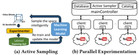
For accurate QoE modeling with ML, we need to have a large training dataset covering the different possible values of the input features. A conventional approach to build such a training set can be to experiment over a large set of unlabeled samples uniformly distributed over the entire experimental space; the space of experi-mentation is given by the range of input features under which the videos are played out. For this study, we consider the following experimental space: 0 − 10 Mbps for bandwidth, 0 − 1000 ms for RTT and 0 − 3 Mbps for the video bitrates taken from the webm video catalog (Fig. 3b). The challenge here is in the large space to cover and the non-negligible time required by each experiment to complete. In order to improve this time and experiment in use-ful regions of the space to build the model quickly, we use active learning, [15], [4]. Active learning is a semi-supervised machine learning approach where the ML model under construction intelli-gently selects which unlabeled samples it wants to label and learn from as part of an iterative process. In our case, labeling refers to the process of experimentation and measuring the QoE. Unlabeled samples are the tuples of the network QoS and video bitrate for which the corresponding QoE label, acceptable/unacceptable, is to be obtained through controlled experiments. In active learning, the ho-mogeneity of the experimental space is exploited by the uncertainty of the model under construction. The objective is to experiment in those regions of the space where the model has high uncertainty
Machine Learning Model
Sample the space intelligently
Re-train and update the model
Labeled Training Set Experimenter RTT DL Bandwidth Video Bitrate
(a) Active Sampling
20
mainController
client client … client
tc
Database Active Sampler
tc tc
Catalog
(b) Parallel Experimentation
Figure 6: The Controlled Experimentation Framework
(quantified by entropy), for example near the current decision bound-ary for a given ML model. In such regions the ML model under construction has low confidence in its prediction (or classification). The intuition is that by experimenting in regions where a transition in the output labels takes place, there is a greater chance of altering the shape of the boundary faster and thus making the ML model converge quickly compared to the case of where experimentations are carried out away from the decision boundary where the labels do not vary. Using this approach, an accurate model can be built faster with fewer experiments.
In order to directly pick a sample in the feature space from re-gions of uncertainty, the space has to be cut into rere-gions which can be done by using algorithms such as Decision Trees (DT). DTs intrinsically split the feature space into regions called leafs. Each leaf has a certain number of samples from each class –the possi-ble output QoE labels– and is labeled with the class having the maximum number of samples in it. Labeled leafs come with some uncertainty, which can be quantified by the measure of entropy. In our approach, we pick a region or leaf for experimentation with a probability that is proportional to the entropy of the leaf. From this selected leaf, we randomly select a feature combination for experimentation. So at each experiment, the underlying DT ML model selects an unlabeled sample from the uncertain leafs, obtains its label by experimention, updates the training set with the labeled sample and finally re-trains the model to complete one iteration. An overall summary of our approach can be visualized in Fig. 6a.
An important question is when to stop the experiments. In our methodology, we stop the experiments when the DT model con-verges to a stable state. The convergence of the DT model can be gauged by a Weighted Confidence measure that quantifies the quality of the model in terms of its classification probabilities. This measure is computed by taking a weighted sum of the entropies of all the leafs of a DT. The weights are assigned to each leaf according to the geometric volume it covers in the feature space. Thus, bigger regions have greater weights and vice versa. So, at each experiment we compute the weighted confidence per class for the DT model and stop experimenting when the standard deviation of this mea-sure over consecutive experiments is within 1% of the average for each class (two classes acceptable/unacceptable in our case).
To further speed up our process of building our dataset, we rely on parallel experimentation. We propose a framework where the logic of choosing the features to experiment with (network QoS and video bitrate) is separated from the client that performs the experiments. With this functional segregation, we are able to have multiple clients running in parallel that ask the central
(a) The Weighted Confidence (b) Cross Validated F1-Score
Figure 7: Model convergence for the DT Model per class
node (mainController) for the network QoS and the video ID to experiment with. After completion of an experiment, the results obtained by each client are sent back to the mainController which updates the central database with the labeled sample and re-trains the active learner. The overall framework is given in Fig. 6b. This setup can be realized in terms of separate virtual machines within the same network or separate physical machines. A benefit of our framework is that the clients do not need to be at the same physical location, they can be geographically separated provided that they are able to communicate with the mainController over the Internet. We apply our proposed framework in a network of 11 physical machines in our experimental platform [16] where the mainCon-troller is hosted on a unique machine while the experiments are per-formed in parallel on the rest of the 10 machines. Our active learning algorithm ended up converging after 2200 experiments. During all these experiments, we had ensured that a large bandwidth and low RTT (less than 10 ms) was available towards the YouTube cloud such that the network degradation was mainly caused by tc.
3.3
Learner convergence and accuracy
Fig. 7 shows the DT model’s convergence. As we can see in Fig. 7a, the model achieves stable confidence value of more than 90% for both classes. To validate the accuracy of the DT-based ML model trained with the QoS-QoE dataset, we rely on usingk-fold cross validation. Ink-fold cross validation, the target dataset is split into training and validation setsk times randomly. The model is then trained with the training set and tested with the validation setk times to getk accuracy scores. The final accuracy score is then the average of thesek scores. We plot the F1-Score1based on cross validation (k = 3 with a data split ratio of 80:20 for training and validation) and updated at each iteration in Fig. 7b. Notice the slight decreasing trend in the cross-validation accuracy compared to confidence that remains stable. The reason for it is that as we keep experimenting, more and more scenarios will be picked from the uncertain regions nearby the boundary between classes, thus making the resulting dataset more and more noisy and difficult to capture the QoE.
3.4
The QoS-QoE dataset
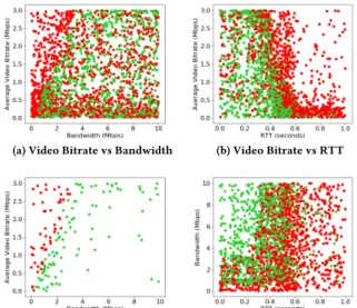
The visualization of the obtained dataset is given in the form of a scatter plot over two dimensions in Fig. 8. The respective colors represent the corresponding classes. The green points represent
1The F1-score is a measure to gauge the accuracy of the ML model by taking into
account both the precision and recall. It is given by2pr /(p + r ), where p and r are the precision and recall of the ML model respectively. It takes its value between 0 and 1 with larger values corresponding to better classification accuracy of the model.
those experiments where the videos play out smoothly (acceptable QoE) while the red points correspond to unacceptable QoE. From Fig. 8a, we can see a relationship between the video bitrate and the downlink bandwidth. As we increase the video bitrate, the required bandwidth to ensure smooth playout increases. Similarly, for latency, as we increase the RTT, more and more videos move from acceptable to unacceptable (Fig. 8b). Notice that the distribution of the points is non-uniform as a consequence of active learning that causes experiments to be carried out with feature combinations near the decision boundary in the feature space. To better illustrate this decision boundary, Fig. 8c is a scatter plot of the data filtered for RTT less than 100 ms from which we can observe a quasi-linear decision boundary between the two classes. Finally from Fig. 8d, we can see that all video playouts are smooth for a bandwidth higher than 4 Mbps and RTT lower than 300 ms. This means that YouTube videos (having resolutions less than or equal to 1080p according to our catalog) can play out smoothly if these two conditions on network QoS are satisfied. The dataset is made available at [10].
(a) Video Bitrate vs Bandwidth (b) Video Bitrate vs RTT
(c) Video Bitrate vs Bandwidth (RTT <100 ms)
(d) Downlink Bandwidth vs RTT
Figure 8: Projection of the QoS-QoE Dataset. Red color: Unac-ceptable playout with stalling or long join time. Green color: Acceptable smooth playout.
3.5
Model validation
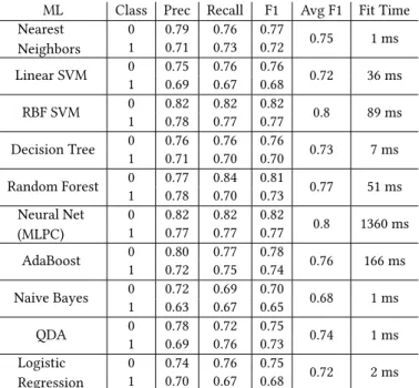
While we use a DT model in our active learning methodology to build the dataset, the resulting QoS-QoE dataset can be used to train other supervised ML algorithms as well. Some ML algorithms such as SVM and neural networks require standardization of data (feature scaling) to perform well. Other classifiers such as Decision Trees and Random Forests do not require such standardization. However, to have a fair comparison, we standardize the dataset and then obtain the cross validation scores for different classifiers. The results are given in Table 2 for default parameter configurations using the Python Scikit-learn library. The best three models are
neural network (Multi-layer Perceptron), SVM (RBF kernel) and Random Forests giving accuracy around 80%.
3.6
Gain of using the Video Bitrate Feature
In order to investigate the gain of using the video bitrate feature in addition to the network QoS features, we train the aforemen-tioned ML algorithms with and without the video bitrate feature. The results for the cross-validation accuracy are given in Table 3. Modeling the QoE using only the network QoS features results in low accuracy of about 65%. This is inline with our earlier re-sult in [4]. However, if we use bitrate with the network QoS, the classification accuracy improves to around 80% giving us a gain of around 15% thus validating the importance of using the video bitrate feature in our QoE modeling scenario.
For our subsequent analysis, we use Random Forests as our pre-dictive QoE model,θ, to devise our global QoE indicator, YouScore, as they do not require standardization on the training data which allows us to use them directly on new data for prediction without any pre processing. They also show good classification accuracy according to Table 2. We can improve their accuracy further by performing a grid search over parameters of min number of samples per leaf and number of estimators; by doing so, we obtain an accu-racy of around 80% with values of 15 and 25 for these parameters respectively. Note here thatθ takes as input the features of RTT, downlink bandwidth and video bitrate (representing the network QoS and the video content) with as output an estimation of the binary QoE (acceptable/unacceptable), while the derived YouScore will only take as input the RTT and downlink bandwidth to give as output an estimate of the ratio of videos that play out smoothly for a given network QoS.
4
YOUSCORE: A QOE INDICATOR FOR
YOUTUBE
Usingθ, we define YouScore, a global QoE indicator for YouTube that takes into account the different video contents of our catalog. Theoretically, we aim to give a probability for YouTube videos of a given resolution to play out smoothly, for a given state of network QoS quantified by the tuple of downlink bandwidth and latency (RTT). To obtain such a probability, we testθ over all the videos in the given catalog and use the model’s predictions to compute the final QoE score ranging from 0 to 1. Such a QoE score inherently contains meaningful information for network operators to gauge their performance w.r.t YouTube, where a score ofx for a given network QoS and for a given resolution translates into an estimated x% of videos of that resolution that would have acceptable QoE (start within 10 seconds and play out smoothly). Formally, we define YouScore for a given resolution r and a network QoS as:
YouScorer = fθ(bandwidth, RTT ). (1) The functionfθ(bandwidth, RTT ) is computed by testing θ with a
test set Tr = {< bandwidth, RTT,bitratei >}i=1Nr composed ofNr
samples of same bandwidth and RTT while the values forbitratei
are taken from the video catalog (composed ofNr videos) for reso-lutionr. To elaborate further, let Yr denote the set of predictions ofθ for Trand Yracceptable ⊆ Yr denote the set of acceptable pre-dictions in Tr. So the final score is given below, which is the ratio
ML Class Prec Recall F1 Avg F1 Fit Time Nearest Neighbors 0 0.79 0.76 0.77 0.75 1 ms 1 0.71 0.73 0.72 Linear SVM 0 0.75 0.76 0.76 0.72 36 ms 1 0.69 0.67 0.68 RBF SVM 0 0.82 0.82 0.82 0.8 89 ms 1 0.78 0.77 0.77 Decision Tree 0 0.76 0.76 0.76 0.73 7 ms 1 0.71 0.70 0.70 Random Forest 0 0.77 0.84 0.81 0.77 51 ms 1 0.78 0.70 0.73 Neural Net (MLPC) 0 0.82 0.82 0.82 0.8 1360 ms 1 0.77 0.77 0.77 AdaBoost 0 0.80 0.77 0.78 0.76 166 ms 1 0.72 0.75 0.74 Naive Bayes 0 0.72 0.69 0.70 0.68 1 ms 1 0.63 0.67 0.65 QDA 0 0.78 0.72 0.75 0.74 1 ms 1 0.69 0.76 0.73 Logistic Regression 0 0.74 0.76 0.75 0.72 2 ms 1 0.70 0.67 0.68
Table 2: Cross Validation scores for common ML algorithms with standardization (k = 10 with a test set size equal to 20% of training set). Class 0: Unacceptable. Class 1: Acceptable.
Features NN RF SVM RTT, DL_BW, Bitrate 0.795 0.784 0.799 RTT, DL_BW 0.667 0.647 0.658 Table 3: Performance gain with the video bitrate feature
of the number of videos to play out smoothly to the total number of videos in the catalog for resolutionr:
YouScorer = | Y
acceptable
r |
Nr (2)
A single score can be computed by taking a weighted sum such thatYouScoref inal = PRr =1wrYouScorer, whereR is the number of resolutions covered in the video catalog andwr can be chosen to give a preference to each of the resolutions.
Using this methodology, we obtain theYouScorer for each reso-lutionr and plot it in terms of heat maps in Fig. 9. The plots are a billinear interpolation of the YouScores obtained at sampled points in the space of RTT and bandwidth: 11 uniformly spaced points on each axis resulting in a total of 121 points. The colors represent the YouScores ranging from zero to one. As we can see, the thresh-olds of bandwidth and RTT where the transitions of the score take place clearly show an increasing trend as we move from the lowest resolution 480p to the highest resolution 1080p. For example, the YouScore begins to attain a value of 1 for bandwidth of around 1 Mbps for 480p, 1.5 Mbps for 720p and 2.5 Mbps for 1080p for RTT less than 200 ms. This threshold also varies on the RTT axis as well.
(a) 480p (b) 720p (c) 1080p
Figure 9:YouScorer usingθ for different resolutions
(a) Science & Technology (b) People & Blogs (c) Sports
Figure 10:YouScore1080p(cateдory)usingθ for different categories
For 240p (not shown here to save space), high YouScores are ob-served for an RTT less than around 500-600 ms. The same threshold reduces to less than 400 ms for resolution 1080p.
To illustrate the variation in the YouScores across different cat-egories, the modelθ is tested over a sampled video set from each category. The resulting scores are given in Fig. 10 for the resolution 1080p. We can see a difference in the scores obtained between dif-ferent categories. Consider the "Science & Technology" category, which has a greater spread. This category gets higher scores com-pared to categories such as "Sports" in the region of low bandwidth and low RTT. From another angle, for low RTT, "Science & Technol-ogy" videos obtain aYouScore1080pof 0.5 at bandwidth of around 2 Mbps, while for "Sports" videos, a higher bandwidth of 3 Mbps is required to achieve the same score. This means that at a bandwidth of 2 Mbps, 50% of "Science & Technology" videos can still play out smoothly whereas no "Sports" videos can play out smoothly at the same bandwidth.
In a practical setting where the global YouScores per resolution need to be computed quickly for a large set of network measure-ments, we can simply use an interpolation function on the sampled points of Fig. 9. To this end, we store these sampled points in a text file which can be retrieved from [10]. Each line in this file represents a mapping of the tuples of RTT (in milliseconds) and Bandwidth (in kbps) to the correspondingYouScore for each resolution.
Our proposed YouScore model (Eq. 1) has the benefit that it re-quires only two out-of-band features of bandwidth and delay to estimate the QoE without requiring the application traffic. Such a model can be easily deployed by a network provider to gauge its per-formance w.r.t YouTube given the available network measurements. Also, we can use as input to the model, the active measurements carried out by crowd-sourced applications such as SpeedTest to es-timate the YouTube QoE; in the next section we demonstrate such a use case.
open_uuid country_location client_version open_test_uuid download_kbit network_mcc_mnc
time_utc upload_kbit network_name cat_technology ping_ms sim_mcc_mnc
network_type lte_rsrp nat_type
lat lte_rsrq asn
long server_name ip_anonym loc_src test_duration ndt_download_kbit loc_accuracy num_threads ndt_upload_kbit
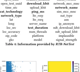
zip_code platform implausible gkz model signal_strength Table 4: Information provided by RTR-NetTest
(a) Scatter Plot (b) Density Map
Figure 11: Downlink Bandwidth vs RTT for RTR-NetTest dataset
5
APPLICATION OF THE YOUSCORE ON
REAL USER NETWORK MEASUREMENTS
In this section, we demonstrate a practical application of YouScore on a dataset of real user active measurements. We use an open dataset of network measurements performed by RTR-NetTest [5], an application developed by the Austrian Regulatory Authority for Broadcasting and Telecommunications (RTR). This application informs users about the current service quality (including upload and download bandwidth, ping and signal strength) of their Internet connection. The dataset is provided on a monthly basis; in our analysis, we use the data for the month of November, 2017. The dataset consists of more than 200k measurements from users mostly in Austria using Mobile, Wifi and Fixed line access technologies. The fields provided in the dataset are shown in Table. 4; details can be found in [5]. Importantly for us, the dataset includes measurements for downlink throughput (estimated bandwidth) and latency, which are required by the function in Eq. 1 to obtain theYouScorer for resolutionr ranging from 240p to 1080p. Specifically, for Downlink bandwidth, we use the value given by the ratio of download_kbit and test_duration, and for RTT, we use ping_ms as input to the function in Eq. 1 to obtain the predictedYouScores.
The visualization of the network measurements is given in Fig. 11a over a limited scale of upto 10 Mbps for throughput and 1000 ms for RTT. In the dataset, the maximum observed throughput (estimated bandwidth) was 200 Mbps while maximum RTT went upto 3000 ms. However bulk of the measurements had smaller values, so we plot here the results over a smaller axis. Notice here the inverse relationship between the download throughput and the latency
4G 3G 2G LAN WLAN YouScore240p 0.97 0.82 0.05 0.93 0.92 YouScore360p 0.95 0.76 0.04 0.89 0.88 YouScore480p 0.92 0.65 0.02 0.83 0.83 YouScore720p 0.82 0.43 0.01 0.68 0.67 YouScore1080p 0.68 0.22 0.01 0.51 0.49 # measurements 28572 6207 723 116617 85879 Table 5: Average YouScores w.r.t Network Technology for the entire dataset
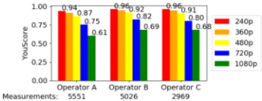
which is an obvious consequence of queuing in routers and of TCP congestion control. For higher RTT values, throughput is always low which signifies that high RTT alone can become a significant factor alone to predict poor QoE for TCP based applications. The same observation can be observed inYouScores (Fig. 9) as well where for RTT higher than 600 ms, the scores are zero for all res-olutions. To visualize the density of the measurements, we plot a heat map in Fig. 11b showing that most measurements have RTT less than 100 ms and bandwidth varies in the range of 0 to 4 Mbps. We now use Eq. 1 to translate these QoS measurements into the correspondingYouScores. The resulting scores are analyzed at the global granularity of cat_technology and network_name. As this dataset also provides the network names for measurements made in mobile networks, we then split the scores w.r.t to different operators to perform a comparative analysis. The overall perfor-mance of each network technology is shown in Table. 5 where we can see an obvious declining trend in the scores as we increase the resolution. The scores for 2G are mostly zero as expected while we get non-zero values for other technologies. The highest score is obtained in 4G for all resolutions. For measurements with mobile technologies, the network names are provided which allow us to dig further to compare the performance between operators. Fig. 12 shows the averageYouScores for top 3 network operators (names are anonymized to ensure unbiasedness). For 240p resolution, the performance is mostly similar among the three but for higher reso-lutions, a difference becomes evident. Using this information, it can be said that a particular operator performs better than the other in providing better YouTube QoE to its end users.
Figure 12: Overall Average YouScores for Top three Network operators for all Radio Access Technologies
Table 6 provides the scores for each radio access technology for the given operators where we can indeed see a difference in the scores across the different operators and across the different technologies. Notice that the highest score forYouScore1080p is 0.77. Our work is limited to 1080p, for even higher resolutions,
Operator RAT count Y360p Y480p Y720p Y1080p
A 2G 20 0.02 0.01 0.00 0.00 A 3G 1012 0.76 0.63 0.39 0.19 A 4G 4486 0.95 0.93 0.84 0.71 B 2G 88 0.03 0.01 0.00 0.00 B 3G 789 0.92 0.85 0.63 0.35 B 4G 4097 0.97 0.95 0.88 0.77 C 2G 42 0.03 0.01 0.00 0.00 C 3G 168 0.85 0.76 0.50 0.29 C 4G 2731 0.97 0.93 0.84 0.72 Table 6: Split of YouScores w.r.t Radio Access Technology (RAT) for top three operators
the scores would be even less. The analysis in this section can be enhanced further by looking at the geographic locations where the measurements are performed. This can help operators prioritize troubleshooting based on the given YouScores. Also, currently, open coverage maps that provide information such as signal strength, throughputs, delay etc are getting common. Such maps can be enhanced with YouScore, to estimate YouTube QoE as well.
6
RELATED WORK
Regarding YouTube catalog analysis, authors in [19] crawled the YouTube site for an extended period of time and performed video popularity and user behavior analysis for a large number of videos. In our work, we take a similar approach based on crawling YouTube to get a statistical insight into YouTube video bitrates but addition-ally we combine this information with QoE modeling as well. From a networking point of view, video QoE has also been studied ex-tensively in literature as well. Recently, authors in [2] model video QoE for encrypted traffic using network level measurements from a dataset of 390k measurements collected on a web proxy of a net-work operator. In [20], a dedicated application to monitor YouTube QoE from mobile devices is presented. In this paper, we provide a different perspective into video QoE where we aim to highlight the variation in QoE due to different contents of the target catalog while scanning the space of network QoS.
A comparison of the accuracy of the QoS-QoE models devel-oped in prior work with our binary modelθ –which is the basis of YouScore– is given in Table 7. The cross validation accuracy for θ is comparable but slightly lower because our dataset has more samples from noisy regions of space due to active sampling. Fur-thermore, the model we present here uses only two QoS metrics enforced on tc (Out-of-band measurements) along with the video bitrate as input features whereas the models presented in the litera-ture mostly use a greater number of QoS fealitera-tures directly obtained from the application traffic itself (In-band measurements). Having more features directly from traffic traces naturally gives better cor-relation with the output QoE, thus normally should result in better models; in a prior work [21], a gain of about 15-20% was achieved by using in-band features for YouTube QoS-QoE modeling with one video. Their drawback, however, is that they require access to the application traffic to predict the QoE, whereas with our out-of-band QoS features, we can talk about QoE prediction without the need to run the application itself or have its traffic.
Related Work QoE Definition Accuracy # Features Type of Features # Training Prometheus [17] Binary (Buffering Ratio > 0.1) 84% ∼36 In-band (traffic traces) 1464 Dimopoulos et. al [2] 3 classes 93% 4 (reduced from 70) In-band (traffic traces) 390,000
Orsolic et. al [18] Binary 89% 9 In-band (traffic traces) 1060 Binary Modelθ Binary (no/low stall/join time) 80% (93% conf.) 3 Out-of-band (tc) 2268
Table 7: A Performance comparison between QoE models that take network QoS features as input
Regarding mobile network performance analysis using crowd-sourced data, authors in [22], [23] present cellular network perfor-mance studies using data collected from devices located through-out the world. In our work, we propose to use such network QoS datasets to compare and benchmark performance of mobile net-works for video QoE using QoS-QoE predictive models.
7
LIMITATIONS
We considered smooth play video play out to be defined to have a join time of less than 10 seconds without any stallings. This is by no means a final definition for smooth play out, rather we only use it as a possible use case for showcasing our methodology for comparative analysis of the performance of cellular networks w.r.t video streaming. We can have different and more complex subjec-tive QoE definitions, but overall our proposed methodology for benchmarking remains the same. Furthermore, the results obtained in Fig. 5 for different mobile operators are highly dependent on the model used and are also not a final representation of the state of today’s mobile networks. In terms of generalization, there is still room to refine YouScore further by using a much larger catalog and use all available resolutions (going upto 4K) and new videos types (such as 3D) that are supported by today’s content providers. Also, our work focuses on one version of Google Chrome on Linux based machines and for webm videos only. The model can be improved further by considering other browsers and mobile devices as well. Finally, the work in this paper is based on YouTube, but our overall methodology is reusable to define global QoE scores for any video streaming system.
8
CONCLUSION
In this paper, we presented a structured approach for performance benchmarking of mobile nerworks for video streaming considering the diversity in the content of the videos in today’s content provider systems. Overall, we started by first collecting a large video catalog for a case of YouTube, then used this catalog to build a QoE model to derive a global QoE Score for the target catalog (YouScore) and finally apply the global QoE score on a dataset of real user network measurements to get a global visibility into the performance of mo-bile networks w.r.t video streaming. Our methodology allows both the network and the content providers to gauge their performance w.r.t video QoE and network QoS respectively.
REFERENCES
[1] T. Hoßfeld, M. Seufert, M. Hirth, T. Zinner, P. Tran-Gia, and R. Schatz, “Quan-tification of youtube qoe via crowdsourcing,” in Multimedia (ISM), 2011 IEEE International Symposium on, Dec 2011, pp. 494–499.
[2] G. Dimopoulos, I. Leontiadis, P. Barlet-Ros, and K. Papagiannaki, “Measuring video qoe from encrypted traffic,” in Proceedings of the 2016 Internet Measurement Conference, 2016, pp. 513–526.
[3] R. K. P. Mok, E. W. W. Chan, and R. K. C. Chang, “Measuring the quality of experience of http video streaming,” in 12th IFIP/IEEE Int’l Symp. on Integrated Network Management, May 2011, pp. 485–492.
[4] M. J. Khokhar, N. A. Saber, T. Spetebroot, and C. Barakat, “On active sampling of controlled experiments for qoe modeling,” in Proceedings of the Workshop on QoE-based Analysis and Management of Data Communication Networks, ser. Internet QoE ’17. ACM, 2017.
[5] “RTR-Netz open dataset,” 2017, https://www.netztest.at/en/Opendata. [6] “MobiPerf - M-Lab,” 2018, https://www.measurementlab.net/tests/mobiperf/. [7] J. De Vriendt, D. De Vleeschauwer, and D. C. Robinson, “Qoe model for video
delivered over an lte network using http adaptive streaming,” Bell Labs Technical Journal, vol. 18, no. 4, pp. 45–62, 2014.
[8] F. Wamser, P. Casas, M. Seufert, C. Moldovan, P. Tran-Gia, and T. Hossfeld, “Modeling the youtube stack: From packets to quality of experience,” Computer Networks, vol. 109, no. Part 2, 2016.
[9] “VP9 Codec,” 2018, https://www.webmproject.org/vp9/.
[10] “Datasets,” http://www-sop.inria.fr/diana/acqua/datasets/YouScore/. [11] “Linux Traffic Control,” 2018, http://lartc.org/.
[12] ITU, “Parametric bitstream-based quality assessment of progressive download and adaptive audiovisual streaming services over reliable transport,” ITU-T Rec. P.1203, 2017.
[13] S. S. Krishnan and R. K. Sitaraman, “Video stream quality impacts viewer behavior: Inferring causality using quasi-experimental designs,” in IMC ’12. ACM, 2012, pp. 211–224.
[14] F. Dobrian, V. Sekar, A. Awan, I. Stoica, D. Joseph, A. Ganjam, J. Zhan, and H. Zhang, “Understanding the impact of video quality on user engagement,” SIGCOMM CCR, vol. 41, no. 4, Aug. 2011.
[15] B. Settles, “Active learning literature survey,” University of Wisconsin Madison, Computer Sciences Technical Report 1648, 2010.
[16] “R2Lab,” 2017, https://r2lab.inria.fr/index.md.
[17] V. Aggarwal, E. Halepovic, J. Pang, S. Venkataraman, and H. Yan, “Prometheus: Toward quality-of-experience estimation for mobile apps from passive network measurements,” in HotMobile ’14. ACM, 2014.
[18] I. Orsolic, D. Pevec, M. Suznjevic, and L. Skorin-Kapov, “Youtube qoe estimation based on the analysis of encrypted network traffic using machine learning,” in 2016 IEEE Globecom Workshops, Dec 2016.
[19] X. Che, B. Ip, and L. Lin, “A survey of current youtube video characteristics,” IEEE MultiMedia, vol. 22, no. 2, pp. 56–63, Apr 2015.
[20] M. Seufert, N. Wehner, F. Wamser, P. Casas, A. D’Alconzo, and P. Tran-Gia, “Unsupervised qoe field study for mobile youtube video streaming with yomoapp,” in QoMEX, May 2017, pp. 1–6.
[21] M. J. Khokhar, T. Spetebroot, and C. Barakat, “An online sampling approach for controlled experimentation and qoe modeling,” in ICC 2018 IEEE International Conference on Communications, 2018.
[22] A. Nikravesh, D. R. Choffnes, E. Katz-Bassett, Z. M. Mao, and M. Welsh, “Mo-bile network performance from user devices: A longitudinal, multidimensional analysis,” in Proceedings of PAM 2014, 2014, pp. 12–22.
[23] S. Rosen, H. Yao, A. Nikravesh, Y. Jia, D. Choffnes, and Z. M. Mao, “Demo: Mapping global mobile performance trends with mobilyzer and mobiperf,” in Proceedings of MobiSys ’14. New York, NY, USA: ACM, 2014, pp. 353–353.