HAL Id: hal-01496397
https://hal.sorbonne-universite.fr/hal-01496397
Submitted on 27 Mar 2017
HAL is a multi-disciplinary open access
archive for the deposit and dissemination of
sci-entific research documents, whether they are
pub-lished or not. The documents may come from
teaching and research institutions in France or
abroad, or from public or private research centers.
L’archive ouverte pluridisciplinaire HAL, est
destinée au dépôt et à la diffusion de documents
scientifiques de niveau recherche, publiés ou non,
émanant des établissements d’enseignement et de
recherche français ou étrangers, des laboratoires
publics ou privés.
near-surface atmosphere at Dome C, Antarctic Plateau
Christophe Genthon, Luc Piard, Etienne Vignon, Jean-Baptiste Madeleine,
Mathieu Casado, Hubert Gallée
To cite this version:
Christophe Genthon, Luc Piard, Etienne Vignon, Jean-Baptiste Madeleine, Mathieu Casado, et
al.. Atmospheric moisture supersaturation in the near-surface atmosphere at Dome C, Antarctic
Plateau. Atmospheric Chemistry and Physics, European Geosciences Union, 2017, 17 (1), pp.691
-704. �10.5194/acp-17-691-2017�. �hal-01496397�
www.atmos-chem-phys.net/17/691/2017/ doi:10.5194/acp-17-691-2017
© Author(s) 2017. CC Attribution 3.0 License.
Atmospheric moisture supersaturation in the near-surface
atmosphere at Dome C, Antarctic Plateau
Christophe Genthon1, Luc Piard1, Etienne Vignon1, Jean-Baptiste Madeleine2,3, Mathieu Casado4, and Hubert Gallée1
1Univ. Grenoble Alpes, CNRS, IRD, IGE, 38000, Grenoble, France
2Sorbonne Universités, UPMC Univ. Paris 06, UMR 8539, Laboratoire de Météorologie Dynamique (IPSL),
75005, Paris, France
3CNRS, UMR 8539, Laboratoire de Météorologie Dynamique (IPSL), 75005, Paris, France 4LSCE-IPSL, CEA-CNRS-UVSQ-U. Paris-Saclay, Gif-sur-Yvette, France
Correspondence to:Christophe Genthon (christophe.genthon@univ-grenoble-alpes.fr) Received: 24 July 2016 – Published in Atmos. Chem. Phys. Discuss.: 18 August 2016 Revised: 7 December 2016 – Accepted: 18 December 2016 – Published: 13 January 2017
Abstract. Supersaturation often occurs at the top of the tro-posphere where cirrus clouds form, but is comparatively un-usual near the surface where the air is generally warmer and laden with liquid and/or ice condensation nuclei. One excep-tion is the surface of the high Antarctic Plateau. One year of atmospheric moisture measurement at the surface of Dome C on the East Antarctic Plateau is presented. The measurements are obtained using commercial hygrometry sensors modified to allow air sampling without affecting the moisture content, even in the case of supersaturation. Supersaturation is found to be very frequent. Common unadapted hygrometry sensors generally fail to report supersaturation, and most reports of atmospheric moisture on the Antarctic Plateau are thus likely biased low. The measurements are compared with results from two models implementing cold microphysics parame-terizations: the European Center for Medium-range Weather Forecasts through its operational analyses, and the Model At-mosphérique Régional. As in the observations, supersatura-tion is frequent in the models but the statistical distribusupersatura-tion differs both between models and observations and between the two models, leaving much room for model improvement. This is unlikely to strongly affect estimations of surface sub-limation because supersaturation is more frequent as temper-ature is lower, and moisture quantities and thus water fluxes are small anyway. Ignoring supersaturation may be a more serious issue when considering water isotopes, a tracer of phase change and temperature, largely used to reconstruct past climates and environments from ice cores. Because
ob-servations are easier in the surface atmosphere, longer and more continuous in situ observation series of atmospheric su-persaturation can be obtained than higher in the atmosphere to test parameterizations of cold microphysics, such as those used in the formation of high-altitude cirrus clouds in mete-orological and climate models.
1 Introduction
Ice supersaturation is frequently found in the upper tropo-sphere (Spichtinger et al., 2003), and specific cloud micro-physics parameterizations are developed to represent this process in meteorological and climate models. These mod-els need to be validated against observations to reproduce cirrus and other clouds including contrails, which develop at altitudes where supersaturation occurs (e.g., Rädel and Shine, 2010). Radiosondes provide snapshot information but obtaining in situ observation time series to comprehensively calibrate and validate such parameterizations is a challenge because it requires flying and operating instruments on high-altitude aircrafts or balloons. Sampling supersaturated air parcels without affecting the air moisture content is also a challenge, as the excess moisture with respect to saturation tends to condense on any surfaces, including those of the sampling device and the sensor itself. There are thus not many in situ observations available to characterize and quan-tify natural supersaturations and their evolution in time, and
evaluate and validate microphysics parameterizations in such conditions.
While they are frequent at high altitude, ice supersatura-tions do not generally occur in the surface atmosphere, where operating instruments is obviously much easier. Atmospheric conditions close to those occurring at the tropopause are, however, found at the surface of the Antarctic ice sheet both in terms of temperature and humidity levels. Because of the distance from the nearest coasts and the high elevation, the Antarctic Plateau is also particularly secluded from sources of aerosols. This is the most likely place on Earth to observe frequent and large ice supersaturation in the near-surface at-mosphere. For instance, Schwerdtfeger (1970) reports on ob-servations of relative humidity with respect to ice exceeding 120 % at Vostok station in the heart of Antarctica.
The possibility of surface atmospheric supersaturation on the Antarctic Plateau raises a potential issue: that of the rel-ative contribution of the different terms of the surface mass balance of the Antarctic ice sheet. The terms are precipita-tion (positive for the surface) and evaporaprecipita-tion/sublimaprecipita-tion (negative or positive), and possibly blowing snow (positive or negative as blown snow redeposits, but generally nega-tive because of enhanced snow evaporation, e.g., Barral et al., 2014). Melting and runoff do not occur on the Antarc-tic Plateau and can be excluded. The net surface mass bal-ance, observed using glaciological methods, is very small on the Antarctic Plateau. It is typically a few centimeters wa-ter equivalent per year (Arthern et al., 2006): the Antarctic Plateau is one of the driest places on Earth. This is because it is so cold, and the laws of thermodynamics indicate that the various terms of the surface mass balance are bound to be correspondingly small. Because they are so small, and be-cause of a harsh environment, the direct determination of precipitation and evaporation/sublimation on the Antarctic Plateau is not conclusive. Their relative contribution to the surface mass balance of the Antarctic Plateau is still poorly quantified, using indirect approaches (Frezzotti et al., 2004). In most places on continents, precipitation largely dominates. This is not necessarily the case on the Antarctic Plateau. In particular, if atmospheric supersaturation occurs near the face, then moisture concentration is likely larger in the sur-face atmosphere than at the snow sursur-face and the turbulent moisture flux is thus directed towards the surface (surface condensation). Unlike most other regions of the Earth, this turbulent flux could contribute positively to the surface water budget and thus, here, on the surface mass balance.
Another potential issue with ice supersaturation on the Antarctic Plateau is that of the impact on the water isotopic composition of snow. Supersaturation leads to kinetic frac-tionation of the stable isotopic composition of water when it condenses. Since the 1980’s (Jouzel et al., 1987), the longest ice core records of past climate and environment are obtained from drilling operations on the Antarctic Plateau. Past atmo-spheric temperatures are deduced from the variations of the concentration of stable water isotopes along the core.
Vari-ations in supersaturation levels may impact kinetic fraction-ation and thus on this reconstruction. Supersaturfraction-ations thus involve not only meteorological (clouds, precipitation, sur-face evaporation/sublimation) but also climate and paleocli-mate reconstruction issues. It is therefore important to mea-sure and assess supersaturations on the Antarctic plateau.
However, as already mentioned, measuring atmospheric supersaturation is a challenge because sampling a super-saturated air mass can affect its moisture content. Schw-erdtfeger (1970) expresses concerns about the reliability of reports of supersaturation at Vostok station. On the other hand, many reports of relative humidity with respect to ice (RHi) on the Antarctic Plateau reach but seem to be
capped at 100 % (King and Andersen, 1999). Genthon et al. (2013) compare RHi observed at Dome C on the
Antarc-tic Plateau, using conventional solid-state sensors, with re-sults from the ECMWF (European Center for Medium-range Weather forecasts) meteorological analyses and from the MAR (Modèle Atmosphérique Régional) meteorological model. In both models, cold microphysics parameterizations are used which, depending on local conditions, allow for su-persaturations (Sect. 4). More often than not, when ∼ 100 % RHi is observed at Dome C with conventional instruments
(not adapted to sample supersaturation), both models pro-duce significant supersaturation, occasionally reaching more than 150 % (Genthon et al., 2013). The cold microphysics parameterizations differ in the two models (see Sect. 4), and other aspects such as the vertical resolution also differ. If both models produce significant supersaturations, they do not quantitatively agree as to the amplitude of the supersatura-tions.
To verify such model results, to decide between and to im-prove the models, using direct is situ measurements, instru-ments must be designed and/or adapted so as to bring the air mass to the moisture sensor without affecting its mois-ture content. This can be done by warming the air above its condensation temperature before ushering it to the sensor. Here, after the present general introduction (Sect. 1), Sect. 2 presents two instruments which are adapted from commer-cial sensors to perform in very cold conditions and to enable the measurement of atmospheric supersaturation at Dome C. The measurement site and deployment are also described in Sect. 2, and previous atmospheric humidity reports from this site are revisited. In Sect. 3, results from the conventional in-struments are compared with the reports by the two adapted instruments and shown to fail. A 1-year climatology of atmo-spheric moisture at Dome C from the adapted instruments is presented, first for summer when both adapted instruments work well but not the unadapted one, then for a full year when instrumental limits occur in the coldest and driest peri-ods and are discussed. The impact of the supersaturations on the turbulent exchange at the surface is calculated and shown to be minor. In Sect. 4, simulation results from recent ver-sions of the two atmospheric models discussed in Genthon et al. (2013) are shown to agree with the observation of
fre-0 500 1000 1500 2000 2500 3000 3500 4000 4500 −180˚ −165˚ −150˚ −135˚ −120˚ −105˚ −90˚ −75˚ −60˚ −45˚ −30˚ −15˚ 0˚ 15˚ 30˚ 45˚ 60˚ 75˚ 90˚ 105˚ 120˚ 135˚ 150˚ 165˚ C
Figure 1. Topographic map of Antarctica, showing the location of Dome C (red C). Elevation (color scale) is in meters.
quent occurrences of supersaturation at all times in the year including in summer. It is also shown that details of the cli-matology and the statistics of occurrence of supersaturation differ between the models and the observations and between the two models. Section 5 discusses the results, issues related to limited ability of models to properly account for supersat-uration (including potential consequences for the record of isotopic signals in the ice), and finally concludes the paper.
2 Measurement site, instruments, and observation methods
Dome C (Fig. 1) is one of the main topographic domes on the East Antarctic Plateau. Since 2005, the summit of the dome (75◦060S, 123◦200E, 3233 m a.s.l.) has hosted a per-manently manned station, Concordia, jointly operated by the French and Italian polar institutes (IPEV and PNRA). One of the first Antarctic Meteorological Research Center automatic weather stations (AMRC AWS, https://amrc.ssec.wisc.edu/) deployed in Antarctica, back in the 1980s, was at Dome C. When the actual location of the summit of the dome was later more accurately determined using satellite and aircraft radar altimeters in the 1990s, the AWS was moved about 50 km to its present position. This induced a 30 m rise and correspond-ingly slight mean surface pressure change but otherwise lit-tle impacted on the series consistency because the local en-vironment is very homogeneous. The AWS provides one of the longest quasi-continuous meteorological reporting on the high Antarctic Plateau. The station measures pressure, tem-perature, and wind, but not moisture. Additional meteorolog-ical reports are available since the construction of Concordia station, including another AWS closer to the station and a daily radiosonde. Both the new station and the radiosondes report atmospheric humidity using solid-state film capacitive
sensors (Kämpfer et al., 2013). In early 2008, a system to vertically profile the lower part of the atmosphere was de-ployed along a ∼ 45 m high tower. Temperature, wind, and moisture are measured, the latter again using solid-state film capacitive sensors. This profiling system is fully described in Genthon et al. (2010, 2011, 2013).
From the tower measurements, Genthon et al. (2013) eval-uate and compare 2 contrasting years, 2009 and 2010, re-spectively the warmest and coldest in a 10-year period. They report measuring humidity up to ∼ 100 % with respect to ice but also observing frequent frost deposition, a hint that su-persaturation occurs but is missed by standard hygrometers without an adaption. Occurrences of supersaturation are fur-ther supported by a comparison with models that implement cold microphysics parameterizations: the models often sim-ulate supersaturation when the hygrometers hit the 100 % RHi ceiling. That raw solid-state hygrometers cannot
mea-sure supersaturation is understandable: a supersaturated air mass will deposit its excess moisture on any hard surface that serves as a condensation surface. The hygrometer body itself will condense the excess moisture before it can be measured. One way to overcome this problem is to aspirate and warm the air above its thermodynamic saturation temperature at the intake.
There are several techniques to measure atmospheric moisture (Kämpfer, 2013). The traditional wet bulb ther-mometer is not very practical, particularly when measuring well below freezing temperature. The dew-point hygrometer provides a direct physical measure of the saturation temper-ature. This is done by progressively cooling a surface from ambient temperature until atmospheric moisture condensa-tion is detected on the surface. The cooled surface is gen-erally a mirror and condensation is optically detected when the reflection of a light beam is observed to be diffused and diffracted. The device also works below freezing temperature but should then be referred to as a frost-point hygrometer (King and Anderson, 1999). Dew and frost-point hygrom-eters are accurate but bulky, complex, and expensive. They require significant amounts of energy, and they have moving parts because the mirror must be periodically cleaned. They are thus comparatively prone to disfunction and failures, and they cannot be used in remote unattended places or in ra-diosondes. On the other hand, they mechanically aspirate air to the sensing mirror, and if the aspiration intake is heated significantly above ambient temperature (such as in King and Anderson, 1999), the measured air is sampled without affect-ing its moisture content, even if supersaturated. Some com-mercial instruments ensure this such as the Meteolabor VTP6 Thygan described below.
In the 1970s, Vaisala Oy (Finland) developed a very dif-ferent, very compact humidity sensor, the Humicap thin-film capacitive sensor1. The dielectric properties and capacitance
1http://www.vaisala.com/Vaisala Documents/Technology
of a polymer film vary with the relative humidity of the ambi-ent air. Although the physical processes for dependence have been described (e.g., Anderson, 1994), the relationship be-tween capacitance and atmospheric moisture is an empiri-cal one. The sensor needs empiri-calibration and a small but signif-icant uncertainty affects the measurement. The uncertainty increases as temperature decreases. On the other hand, the Humicap is convenient, very compact, comparatively inex-pensive, robust, its use can be automated, and it can be de-ployed even in remote places and on radiosondes. It is thus currently widely used for such purposes. Thin-film capacitive sensors are used in all automatic weather stations in Antarc-tica that report moisture as well as on the 45 m profiling sys-tem at Dome C mentioned above, in the latter case bundled in Vaisala HMP155 thermometers–hygrometers (thermohy-grometers) (Genthon et al., 2013). According to the manufac-turer, the uncertainty is ±1.4 + 0.032 of the reading in per-centage in the −60 to −40◦C temperature range. It is smaller
at warmer temperature and may be expected to be larger be-low −60◦C. However, then, the absolute moisture content of the atmosphere is smaller and absolute measurement errors are correspondingly smaller.
To tentatively confirm and quantify supersaturations at Dome C, both frost-point and thin-film capacitive hygrom-eters were deployed at a height of 3 m and adapted as neces-sary to operate in the general Dome C conditions and to sam-ple the air without altering its moisture content, even when above saturation. In both systems, the hygrometer-aspirated intake is heated so that the temperature of the sampled air parcel is raised above condensation level and condensation is avoided. The frost-point hygrometer is a Meteolabor VTP6 Thygan chilled mirror instrument. It was selected because it is factory-designed to perform in cold temperatures and correspondingly low specific humidities. According to the manufacturer the lowest measurable frost-point temperature is −65◦C. The fact that the air is heated at the intake (see below) does not improve the temperature range of the in-strument as the actual limitation is due to the ability to cool the mirror to the condensation temperature. A −65◦C tem-perature limit is not quite low enough to consistently oper-ate at Dome C, where the surface atmospheric temperature can occasionally drop below −80◦C. In addition, the sen-sor was found to begin and increasingly fail below −55◦C rather than −65◦C. However, data from the vertical profil-ing system show that from 2009 to 2015, the air tempera-ture ∼ 3 m above the snow surface was warmer than −55◦C more than 50 % of the time, and almost consistently (more than 99.5 % of the time) warmer than −55◦C during the
lo-cal summer (December–January–February). Assuming near saturation, the instrument can nominally operate for a large fraction of the time at Dome C. For our application, the frost-point hygrometer (denoted as FP from now on) is hosted in a heated box so that the electronics and mechanics are not affected by the extreme cold temperatures in winter. By fac-tory design, the outside air is aspirated inside the instrument
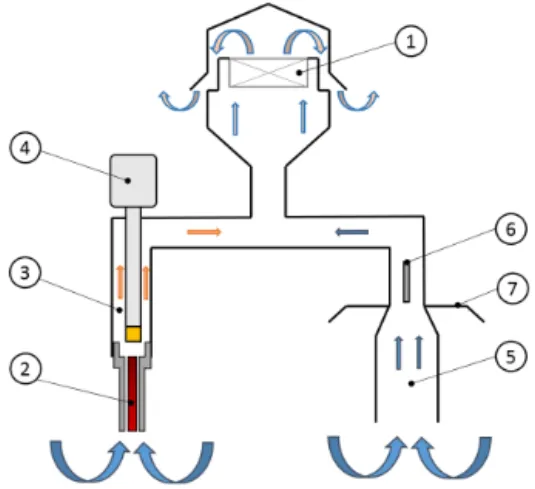
Figure 2. Schematic drawing of the modified (HMPmod) hygrome-ter. The air is aspirated by the fan (1) and heated through an inlet (2). The temperature and the moisture content of the heated air (3) is measured by the HMP155 (4). The ambient air temperature (5) is measured by a separate PT100 (6) located in the unheated aspirated inlet shaded from sun radiation (7).
through an intake protected by a heated hood which prevents frost deposition. This design is not modified, the intake and heated hood being simply made to protrude out of the heated box, to sample the outside air. This is the only part of the instrument outside the heated box and, because it is itself heated, loss of moisture along the way to the mirror is consis-tently prevented. Visual inspection confirms that even when frost deposition occurs on other instruments on the tower, no frost deposition is observed in the vicinity of the instrument intake. Each measurement cycle lasts 10 min: heating and de-frosting the mirror from the previous measurement, cleaning, then cooling until frost point is reached. The sensor thus re-ports measurements of frost-point temperature, and conver-sion to relative humidity, on a 100time-step basis. The manu-facturer claims a very high accuracy: 0.1 % expressed in term of relative humidity. Dew and frost-point hygrometers are in-deed often used to calibrate other types of hygrometers. Here the FP is used as a reference against which other sensors may be adjusted and are evaluated, at least down to temperatures where the FP performs well.
For the other type of hygrometer used here, the manu-facturer (Vaisala Oy) guaranties its HMP155 sensor down to −80◦C for the measurement of temperature, but only to −60◦C for the measurement of moisture. However, the main issue with colder temperatures for this instrument is that the time response increases. Yet, unlike in a radiosonde for which the environment quickly varies during ascent, varia-tions are comparatively slow for fixed instruments and the operational limit is actually much below −60◦C (Genthon et al., 2013). In addition, to avoid frost deposition and preserve the air moisture content, for our application, the instrument aspirates the air through an inlet consistently heated ∼ 5◦C above the ambient temperature (Fig. 2). The ambient
temper-ature itself is measured by a separate PT100 platinum resis-tance thermometer in an unheated derivation of the system. A comparison with the frost-point hygrometer shows that this simple and low-cost innovative design succeeds in measur-ing even highly supersaturated air. In addition, the fact that the air reaching the hygrometer sensor is 5◦C above ambi-ent temperature correspondingly extends the actual nominal temperature range of the instrument with respect to ambient temperature. The sensor reports relative humidity. According to manufacturer, the accuracy in the low temperature range (−60 – −40◦C) is ±1.4 % of the reading. Accuracy improves at warmer temperature, and may conversely be expected to deteriorate for even colder temperatures. The temperature range −40 to −60◦C is typical at Dome C although temper-atures as cold as −80◦C and as warm as −15◦C may be en-countered. Note that in accordance with meteorological con-ventions, all sensors report relative humidity with respect to liquid water rather than ice even when the air temperature is below 0◦C. Goff–Gratch formulas (Goff and Gratch, 1945) are commonly used in meteorology to convert between RH with respect to liquid, water vapor partial pressure, and RHi:
they are also used here. Differences up to 20 % have some-times been reported with alternate formulas in extremely cold temperature ranges. However, because the formula are used here to converted form RH with respect to liquid water to partial pressure then to RHi, the inaccuracies partially
com-pensate.
A potential concern with the heated inlet approach is that, if there are airborne ice particles, they may be aspirated and evaporated in the heated section, leading to a spuriously el-evated water vapor ratio in the sampled air, translating into supersaturation when RHiis recalculated against the ambient
air temperature. Airborne ice particles may result from either blowing snow or occurrence of a cloud. A signature of the bias would thus be that supersaturation magnitude and oc-currence increase with wind speed and/or with downwelling infrared radiation. The reason is that blowing snow occurs if the wind is strong enough to erode and lift snow from the sur-face, while even a very light cloud in such a cold and dry at-mosphere induces a significant increase the IR emissivity and thus of downward IR (Gallée and Gorodetskaya, 2000; Town et al., 2007). In the observations to be presented next, the cor-relations are actually negative. RHi is consistently at or
be-low 100 % for wind speed above 8 m s−1(Fig. 3), which is a typical speed at which blowing snow can be triggered (Libois et al., 2014). Stronger winds are generally associated with air masses originated from the coast and thus comparatively laden with aerosols preventing supersaturation. Supersatura-tions sharply increase rather than decrease in frequency and amplitude with downwelling IR below ∼ 130 W.m−2 char-acteristic of a clear sky (not shown). These results are fair signals that airborne ice particles are not likely to bias the measurements presented here. Caution with the reliability of the most extreme, and less frequent, supersaturation events may nonetheless by recommendable.
LWdn
(W m
−2)
50 100 150 200RH
i(%
)
60 70 80 90 100 110 120 130 140 150 160Figure 3. Scatter plot of observed RHibetween 60 and 160 % (from
HMPmod) versus 10 m wind speed. All available half-hourly data in 2015 are plotted.
The two adapted instruments are deployed side by side ∼3 m above the snow surface on the ∼ 45 m tower. At the same level, hosted in an aspirated but unheated radiation shield (see Fig. 1 of Genthon et al., 2011), an unmodified HMP155 allows for comparison with a traditional design – and to exhibit biases of the latter. From now on, the origi-nal and modified HMP155 will be referred to as “HMP” and “HMPmod”, respectively. Table 1 lists the instruments and adaptations. The various instruments performed over the du-ration of 2015 except for limited periods due to data-logging failures or servicing in summer. The results are presented and analyzed in the next section and compared with models in Sect. 4.
3 Observation data and results 3.1 Summer
Figure 4 displays the mean diurnal cycle of atmospheric moisture and temperature in January, February, and Decem-ber 2015 according to the various instruments. During this period, the FP is consistently running within its nominal manufacturer-stated temperature range and can serve as a moisture measurement reference for the other instruments. The sun never completely sets at this time of the year, however its changing elevation above the horizon induces a strong temperature cycle near the surface (Fig. 4d). Here, “night” refers to the local hours during which sun elevation is lower at Dome C and sets at lower latitudes, broadly the cold-est half of the day. Figure 4a shows the mean cycle of partial pressure of water vapor from FP. The numbers are low due to the cold temperature: the water partial pressure ranges on av-erage between ∼ 15 Pa in the early morning and slightly over
Table 1. List of hygrometers and adaptations. See text for details.
Short name Instrument/sensor Housing
HMP Vaisala HMP155 thermohygrometer/ Aspirated radiation shield
thin-film polymer hygrometer
HMPmod Modified Vaisala HMP155 thermohygrometer/ Aspirated radiation shield
thin-film polymer hygrometer +heated intake (Fig. 2)
FP Meteolabor Thygan VPT6 mirror Heated enclosure, heated intake
frost-point hygrometer 0 4 8 12 16 20 24 15 20 25 30 35 40 Pa 0 4 8 12 16 20 24 -4 -3 -2 -1 0 Pa 0 4 8 12 16 20 24 9095 100105 110115 120 % wri HMP HMPmod FP 0 4 8 12 16 20 24 Local time -42 -40-38 -36 -34 -32 -30 °C (a) (b) (c) (d)
Figure 4. Mean December–January–February diurnal cycle of: (a) water vapor partial pressure from FP instrument; (b) difference with respect to FP of water vapor partial pressure from original (HMP, black) and modified (HMPmod, red) thin-film polymer
sen-sors; (c) RHi from the three instruments; (d) 3 m air temperature.
35 Pa in the early afternoon. This cycle demonstrates that sur-face evaporation occurs during the day, followed by deposi-tion at night, resulting in surface (3 m) atmospheric mois-ture diurnally changing by a factor of more than 2. Figure 4b shows small differences and consistent agreement between the HMPmod and FP instruments. Note here that HMPmod is slightly calibrated for moisture reports against the FP instru-ment for agreeinstru-ment in the early afternoon at the warmest part of the day. This calibration does not exceed manufacturer stated accuracy for HMP155 (Sect. 2). The calibration proves robust and valid at all times during the day in this period. Re-sults from (unmodified) HMP significantly depart from those of the FP, and thus HMPmod instruments: the agreement is good in the afternoon only, but quite poor the rest of the day and at night. Figure 4c displays the calculated RHi for the
three instruments, using the independent moisture measure-ments by each instrument, but all finally reported to one same atmospheric temperature, that of the (unmodified) HMP. This
Figure 5. Regression of anomaly to saturation vapor pressure from HMP (a) and HMPmod (b) instruments against FP.
is likely the most accurate estimation of temperature, i.e., the least-likely affected by radiation and other biases because it is unheated and most efficiently ventilated (Genthon et al., 2011). Temperature differences of as much as 2◦C are oc-casionally observed with the other instruments in low wind conditions.
RHi differs markedly between the unmodified HMP and
the two other instruments. The latter two both report RHi
significantly exceeding 100 % while the unmodified instru-ment hardly reaches saturation. All instruinstru-ments agree well in the early afternoon at the warmest time of the day but HMP disagrees at night. The FP and HMPmod instruments consis-tently agree with each other, including when reporting aver-aged summer supersaturations reaching 120 % at night, con-firming the high levels of supersaturation hinted by Genthon et al. (2013) from models.
Figure 5 displays correlation plots of moisture reports from the unmodified (HMP) and modified (HMPmod) thin-film capacitive sensors with respect to FP in summer. The direct correlations between water vapor pressures would be very high because humidity is largely controlled by temper-ature. Plotting deviations to the saturation vapor pressure, rather than the vapor pressure itself, removes much of the temperature codependence effect and concentrates on the rel-ative ability of the instruments to correctly measure moisture. The correlation between the regular HMP and FP is good below saturation but is obviously very poor above since the HMP fails to capture supersaturations. The correlation be-tween HMPmod and FP reports is very high, above 0.97. The
60 80 100 120 140 % w.r.i. 0 10 20 30 40 50 60 70 % HMP HMPmod FP 60 80 100 120 140 160 180 200 % w.r.i. 0,01 0,1 1 10 (a) (b)
Figure 6. Observed distributions of RHi in 2015 for cases of RHi
between 50 and 150 % with linear vertical RHi scale (a) and
be-tween 50 and 200 % and with logarithm vertical RHi scale (b).
regression constant (the intercept) is 0.1 but the standard er-ror on the constant is larger than 0.1. The linear regression is thus not statistically different from a 1/1 regression. 3.2 Annual variations and statistics
A strong diurnal cycle dominates the variability of atmo-spheric moisture in summer. The partial pressure is maxi-mum in the early afternoon while RHi peaks near local
mid-night (Fig. 4) when it occasionally reaches more than 150 % (not shown). As the diurnal cycle variability progressively vanishes and is replaced by synoptic variability in the colder months, RHi occasionally reaches values above 200 %.
Fig-ure 6 displays the distributions of observed RHiwith the
var-ious instruments, both limiting the range of RHibetween 50
and 150 % (more than 99 % of all HMPmod reports) and ex-tending the range to 200 %. A logarithmic RHi scale is used
in the latter case because with the linear scale the highest RHi values would almost merge with the axis and hardly be
visible.
Although measurement uncertainties and uncertainties on conversions from relative humidity with respect to liquid to RHi allow some occurrences above 100 %, as expected, the
reports from HMP peak near and hardly exceed the 100 % ceiling. More than 50 % of all reports between 50 and 150 % are above 100 % for HMPmod and FP, with similarities of distribution for the two instruments. There are differences between observations by even the two modified hygrometers though. In the 50–150 % range, there are more quantitative differences between the HMPmod and FP below 100 % than above. Both the HMP155 and frost-point hygrometer lose ac-curacy and sensitivity as the temperature is colder and/or
wa-ter vapor partial pressure is lower. Below −55◦C, FP occa-sionally, and more and more frequently as temperature gets colder, reports unrealistically low moisture content. A limit with the colder temperatures for this instrument is reported in Sect. 2. Figure 7 displays the regressions of water vapor par-tial pressure differences with saturation, separately for parpar-tial pressure ranging between 2 and 5, 5 and 10, 10 and 20, and exceeding 20 Pa. The correlation deteriorates, and the regres-sion line increasingly deviates from 1 to 1, as the moisture content decreases.
Obviously, the smallest moisture partial pressures occur when the temperature is coldest. The instruments show their limits during the coldest periods of the winter. Figure 8 dis-plays the annual cycle of monthly-averaged temperature and RHi. HMP displays weak seasonal variability of RHi
com-pared to the other instruments. On the other hand, FP dis-plays extreme seasonal variability with values reaching be-low 30 % (beyond the plot scale in Fig. 8) in winter. Such unrealistically low values, at odds with the other instruments, reflect instrument limitation with very low moisture content. Limiting the analysis to cases of partial pressure of mois-ture above 2 Pa (dashed curves in Fig. 8) excludes signifi-cant portions of the coldest parts of the winter records. This is reflected by monthly winter temperatures more than 20◦C warmer (Fig. 8a). The fact that HMPmod reports are strongly increased suggests that this sensor also does not perform well at very low moisture levels. When restricting to above 2 Pa, both HMPmod and FP show strong seasonal variability with monthly mean RHi reaching 120 % for HMPmod and
ex-ceeding 130 % for FP. In both cases, the maximum monthly supersaturation is reached in early winter (April) and remains above 100 % all year long, except in October for HMPmod when it is slightly below. Figure 9, same as Fig. 6 but for par-tial pressure of moisture above 2 Pa only, confirms that in the surface atmosphere of Dome C, supersaturation is the norm rather than an exception.
3.3 Impact on surface sublimation calculations
There are very few direct estimates of surface evaporation on the Antarctic Plateau. This is firstly because eddy correlation techniques use delicate high-frequency sampling instruments such as sonic anemometers, which are hard to operate and maintain at the required level of performance in the extreme environment of the Antarctic Plateau. Moreover, due to the very low temperature, the water vapor content is very small and moisture sensors are neither fast nor sensitive enough for measurement in such conditions. For instance, Van As et al. (2005) report that eddy correlation measurements of latent heat flux were unsuccessful even in the summer at Kohnen station in Antarctica, ∼ 3000 m above sea level. The authors thus resigned themselves to using bulk methods, a widely employed approach in Antarctica (Stearns and Wei-dner, 1993). However, bulk methods are equally affected by measurement biases such as underestimation of water vapor
Figure 7. Regressions of partial pressure difference with saturation from HMPmod against FP, depending on partial pressure range as indicated on the upper left corner of each plot. The black line is the first bisector, the red line shows the linear regression.
Figure 8. Seasonal variability of monthly-mean temperature Tm
(a) and RHi(b) for all reports (solid lines) and reports with moisture
partial pressure ph above 2 Pa only (dashed lines). With all reports, the curve for FP reaches below 30 %, well beyond the plot scale (green solid line).
content due to failure to measure supersaturation. The mag-nitude of the error can be estimated at Dome C by comparing bulk calculations using HMP and HMPmod water vapor re-ports.
The water vapor flux E from the snow surface (subscript “s”) to the atmosphere is calculated using bulk-transfer for-mulas:
E = ρCQU (z)[qs−q(z)], (1)
where ρ is the air density, U(z) and q(z) are the wind speed and the specific humidity, respectively, at the height z in the atmospheric surface layer, and qs is the specific humidity at
50 60 70 80 90 100 110 120 130 140 150 % w.r.i. 0 10 20 30 40 50 60 70 80 90 % HMP HMPmod FP
Figure 9. Same as Fig. 6 but for moisture partial pressure above 2 Pa only.
the surface, assuming saturation with respect to ice at the snow surface temperature. Here the wind speed and specific humidity are measured at z = ∼ 3 m above the surface, and the snow surface temperature is obtained from measurement of the upwelling infrared radiation (Vignon et al., 2016) con-sidering a snow emissivity of 0.99 (Brun et al., 2011). CQis
a bulk transfer coefficient which is written as follows:
CQ=κ2[ln(z/z0) − ψm(z/L)]−1[ln(z/z0q) − ψq(z/L)]−1, (2)
where κ is the Von Kármán’s constant, z0and z0qthe
rough-ness lengths for momentum and water vapor respectively, and ψm and ψq are the corresponding surface-layer
simi-larity stability functions. Stability functions depend solely on the dimensionless height z/L, where L is the Monin– Obukhov length (Vignon et al., 2016; Stull, 1990). The same four function schemes taken for stable conditions in Vi-gnon et al. (2016) are tested here, and the functions from Hogström (1996) are selected for unstable conditions be-cause they provide reasonable results for momentum and heat fluxes at Dome C (Vignon et al., 2016). L and thus CQare calculated with an iterative resolution of the Monin–
Obukhov equations system. The value of z0is the mean value
reported by Vignon et al. (2016) for Dome C (0.56 mm). The value of z0q is difficult to estimate at Dome C because the
very low vapor content of the atmosphere induces high uncer-tainties and because the scarcity of near-neutral conditions prevents an independent selection of a scheme for the stabil-ity functions. Two different approaches are used. By default, z0q =z0as in King et al. (2001), and in a second case, z0q
is calculated with Andreas (1987) theoretical formula, which at Dome C yields z0q values lower than z0by approximately
Figure 10. Annual march of the monthly vapor flux at the sur-face according to HMP (red) and HMPmod( green), the black line showing 0 (upper plot), and cumulated difference (HMPmod–HMP, lower plot).
are estimated from the variance of results obtained with the different choices of stability functions and roughness length. Figure 10 shows the monthly seasonal water flux calcu-lated by the bulk method for 2015 using either HMP data or HMPmod reports, and also shows the cumulated difference between the two calculations. The flux is positive during the summer months indicating sublimation of snow, while dur-ing winter months the flux is negative, indicatdur-ing conden-sation to the surface. Such seasonality is in agreement with that reported by King et al. (2001) at Halley station, which is situated in coastal Antarctica but at a latitude similar to that of Dome C. The positive summer values reflect the pre-dominance of snow sublimation during the summer diurnal cycle (Genthon et al., 2013) because, in summer, the surface– atmosphere exchanges are larger during convective activity in the afternoon than in the night hours when the boundary layer becomes stable (King et al., 2006; Vignon et al., 2016). Integrated over the full year 2015, the net water vapor flux is 0.2763 cm w.e. using HMPmod data and 0.2863 cm w.e. using HMP data. These numbers can vary by as much as ±100 % with the different choices of stability functions and roughness length values. They are very small anyway com-pared to the total surface water budget, given that the mean annual accumulation is about 2.5 cm w.e. (Genthon et al., 2015). However, a mean positive evaporation agrees with Stearns and Weidner (1993) who, for other regions of Antarc-tica, conclude that the annual-mean net sublimation exceeds the annual-mean net deposition. In fact, Fig. 10 shows very little difference between calculations made with HMP and HMPmod data: the impact of supersaturation on the water heat flux is thus very small. This is because supersaturations predominantly occur when the wind speed and thus turbu-lence are weaker (Fig. 3), and when specific humidity is low (Fig. 11) and thus turbulent flux are weak (Eq. 1). A possible
Figure 11. According to HMPmod, relative humidity versus water vapor partial pressure, saturation shown by the red line (upper plot),
and probability distribution function of RHi above 105 % with
re-spect to water vapor partial pressure (lower plot).
contribution of blowing or drifting snow sublimation (King et al., 2001; Frezzotti et al., 2004; Barral et al., 2014) is not taken into account in the calculations here.
4 Meteorological models and cold microphysics parameterizations
The introduction (Sect. 1) refers to the results of Genthon et al. (2013) showing that two models with cold microphysics parameterizations for water condensation predict significant supersaturation at Dome C. Observations are now available to verify these results and the general models’ ability to sim-ulate the characteristics of supersaturation at Dome C. Model results from both the MAR and ECMWF are again evaluated here, although these are results from “up to date” model ver-sions as of 2015, which differ somewhat from those in Gen-thon et al. (2013).
4.1 Meteorological models and microphysics highlights MAR is a limited area coupled atmosphere–surface model. Atmospheric dynamics are based on the hydrostatic approx-imation of the primitive equations (Gallée and Schayes, 1994). The vertical coordinate is the normalized pressure. Near the surface where observations are made, parameteriza-tion of turbulence in the surface boundary layer is based on the Monin–Obukhov similarity theory and turbulence above the surface boundary layer is parameterized using the K-ε model, consisting of two equations for turbulent kinetic en-ergy and its dissipation. The prognostic equation of dissipa-tion allows one to relate the mixing length to local sources of turbulence and not only to the surface. The K-ε model used here has been adapted to neutral and stable conditions by Duynkerke (1988). The influence of changes in water phases
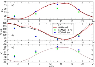
Figure 12. Mean December–January–February diurnal cycle of ob-served (FP and HMPmod) and analyzed (ECMWF, 2 m and first model level at ∼ 8 m) water vapor partial pressure (a), relative hu-midity with respect to ice (b) and temperature (c). The reference temperature is that from the unmodified HMP (brown curve in c).
on the turbulence is included following Duynkerke and Drei-donks (1987). The relationship between the turbulent diffu-sion coefficient for momentum and scalars (Prandtl number) is dependent on the Richardson number following Sukorian-sky et al. (2005).
Prognostic equations are used to describe five water species (Gallée, 1995): specific humidity, cloud droplets and ice crystals, rain drops and snow particles. A sixth equation is added describing the number of ice crystals. Cloud mi-crophysical parameterizations are based on Kessler (1969), Lin et al. (1983), and Levkov et al. (1992). In particular, cloud droplets are assumed to freeze at temperatures below 238.15 kK while contact-freezing nucleation, deposition and condensation freezing nucleation of ice crystals follow the formulation of Meyers et al. (1992) improved by Prenni et al. (2007). Surface processes in MAR are modeled using the soil ice vegetation atmosphere scheme (SISVAT). For the present experiment, MAR is set up over the region of Dome C with a horizontal resolution of 20 km over a 41 × 41 grid. Lateral forcing is taken from ERA-Interim (Dee et al., 2001). There are 15 model levels in the vertical between the surface and 32 m, where temperature and moisture are ex-plicit prognostic variables of the primitive equations and pa-rameterizations.
Numerical weather forecasts are produced by meteoro-logical models initialized with meteorometeoro-logical analyses. Me-teorological analyses are the result of optimally combin-ing (assimilatcombin-ing) meteorological observation from various sources (surface, radiosounding, satellites, etc.) with(in) a meteorological model. Unlike observations, which are scat-tered in time and space, meteorological analyses have the full time and space coverage and resolution of the model. The ECMWF produces global meteorological analyses to
Figure 13. Mean December–January–February diurnal cycle of ob-served (FP and HMPmod for moisture, HMP for temperature) and
MAR-simulated RHi (a) and air temperature (b), the brown curve
being the observed as in Fig. 12.
initialize its forecasts: these are the near real-time opera-tional analyses. Like other weather services, the ECMWF has also produced reanalyses, retrospective analyses for purposes other than real time operational weather forecasts. The ERA-Interim data used as lateral forcing for MAR (see above) are reanalyses produced by ECMWF. Reanalyses are more con-sistent in time than operational analyses because they use the same meteorological model and assimilation package while these are constantly changed towards improvement and finer resolution in the operational analyses. Some changes oc-curred in the ECMWF operational system in the course of 2015 but such major aspects as horizontal and vertical res-olution were not affected. Because the vertical resres-olution is significantly finer near the surface in the operational analy-ses than in the reanalyanaly-ses, we elect to use here the operational analyses to compare with the observations.
The ECMWF model (versions CY40R1 and CY41R1 for the year 2015) is part of the ECMWF IFS (Integrated Fore-casting System). The ECMWF provides a full description on-line2. It is a spectral general circulation model based on the hydrostatic primitive equations. Parameterization in the sur-face boundary layer is again based on the Monin–Obukov similarity theory while turbulent coefficients in the unstable mixed layer above are computed using the eddy-diffusivity mass flux (EDMF) approach (Kohler et al., 2011). They are determined above the mixed layer and in stable conditions using a first-order closure based on the wind shear, a mixing length and the local Richardson number.
The cloud microphysics scheme is described in Forbes et al. (2011). Prognostic equations are used for cloud liquid, cloud ice, rain, and snow water contents. The scheme allows supercooled liquid water to exist at temperatures warmer than the homogeneous nucleation threshold of 235.15 K. At temperatures colder than this, water droplets are assumed to
2http://www.ecmwf.int/search/elibrary/part?solrsort=sort_
labelasc&title=part&secondary_title=40r1, http://www.ecmwf.int/ search/elibrary/part?solrsort=sort_labelasc&title=part&secondary_ title=41r1
freeze instantaneously. For temperatures below the homoge-neous freezing temperature, the scheme also assumes that ice nucleation initiates when local RHi reached a threshold
(Karcher and Lohmann, 2002).
At the surface, the snowpack is treated taking into account its thermal insulation properties and a representation of den-sity (Dutra et al., 2010). The vertical resolution in the atmo-sphere near the surface is not as fine as in the MAR model. The mean elevation of the first prognostic model level at Dome C in summer is 8.2 m, significantly higher than the observation level. Variables are also calculated at the meteo-rological standard 2 m level by interpolation between the first level and the surface using gradient equations of the surface layer. Vignon et al. (2016) show that the surface layer where gradient interpolation relationships are valid is often much shallower than 8 m in stable conditions at Dome C. The 2 m interpolated values probably encompass biases due to the in-terpolation formula and may have to be considered carefully. However, the elevations of the 2 m and first-level data bracket that of the observations, allowing a more detailed compari-son in a region where vertical gradients can be steep. 4.2 Model data comparison
Figure 12 compares the observed diurnal cycles of temper-ature and moisture with the ECMWF analyses at the first model level and at the standard 2 m level. A similar compari-son is shown with MAR at the closest model level in Fig. 13. There are only four analysis steps per day, so ECMWF data are shown as dots in Fig. 12 when the observations (48 data per day) and MAR results (240 per day) are shown as con-tinuous curves in Figs. 12 and 13.
The ECMWF analyses overestimate nighttime tempera-ture and consequently underestimate the amplitude of the di-urnal cycle. The amplitude of the cycle of moisture partial pressure is also underestimated but not as badly as could be expected considering a non-linear relation between temper-ature and saturation humidity. The model thus agrees with a large diurnal change in magnitude and sign of the surface turbulent flux of moisture. The surface atmosphere is expect-edly moister, and the vertical gradient and turbulent flux di-rected upward (surface sublimation) in the early afternoon. It is downward (deposition) and much weaker at night. Be-cause of the temperature errors, RHi is less than observed
at night, yet it is significantly larger than 100 %. The anal-yses reproduce supersaturation at night and minimum RHi
in the early afternoon. MAR also produces large supersat-urations, which are actually larger than the observations in summer (Fig. 13a). However, the model is significantly and consistently too warm (Fig. 13b), which was not the case in the model version used in Genthon et al. (2013). Supersatu-rations are nonetheless a robust feature of this model.
Figure 14 displays the distribution functions of ECMWF-analyzed and MAR-modeled RHi. This is to be compared
with Fig. 6a for the observations. The 2 models are
success-Figure 14. ECMWF-analyzed (a) and MAR-modeled (b)
distribu-tions of RHi in 2015 for cases of RHi between 50 and 150 %. The
fact that a different time sampling in the models (this figure) and the observations (Fig. 6) does not affect the comparison was verified.
ful at reproducing very frequent occurrences of supersatura-tion, however their distributions differ both with the obser-vations and with each other. The MAR model is much more often supersaturated than the observations report, and also than the ECMWF analyses. RHi in the MAR model exceeds
200 % much more often than both the observation and the ECMWF analyses (not illustrated in Fig. 14 for scale reasons as discussed in Sect. 3.2/Fig. 6), raising particular concerns about the treatment of the cold microphysics in this model. Differences between models and between one or the other model and the observations are beyond observation uncer-tainties. Further analyses of these differences, comparing the respective cold physics parameterizations and tracking possi-ble contributions of temperature biases, is beyond the scope of the present study. However, this result illustrates that be-cause long series of consistent in situ observations are feasi-ble at Dome C, not only short term chronology but also the statistics of supersaturation can be quantified and used to ex-hibit differences in behavior of models and parameterizations of natural atmospheric supersaturation.
5 Discussion and conclusions
Major ice supersaturations are observed in the surface atmo-sphere of Dome C on the Antarctic Plateau in atmospheric temperature and moisture conditions that are similar to those of the upper troposphere. To our knowledge it is the first time such strong supersaturations (up to 200 %) are observed in the natural surface atmosphere of the Earth. The presence of high ice supersaturations suggests very low concentrations of ice nuclei (see King and Anderson, 1999). More instru-ments on the tower of Dome C are being considered to detect fogs and monitor their properties, including supercooled wa-ter fogs (see, e.g., Anderson, 1993). This would help
under-standing the microphysical conditions under which these ice supersaturations occur and improve microphysics schemes used in models. Atmospheric supersaturations are frequent in the high troposphere where cirrus clouds form (Spichtinger et al., 2003). On the other hand, atmospheric supersaturation is an infrequent situation in the surface atmosphere because of the high concentration of aerosols and relatively mild tem-peratures which are both favorable to liquid and solid cloud formation. In this respect, the surface atmosphere of the high Antarctic Plateau is a relative exception. Because of the high albedo of snow, high latitude, and high elevation, the temper-ature and humidity are close to that of the high troposphere elsewhere even in summer. Long-distance transport to such a remote area is insufficient to import significant amounts of cloud and ice condensation nuclei even from the closest sources at the oceans, thus the possibility of strong and fre-quent supersaturation.
Conditions for surface supersaturation may be found else-where in the polar regions. King and Anderson (1999) ob-served supersaturations of 150 % or more, and a significant frequency of ice supersaturation of 120 % or more, at the coastal Antarctic station Halley. Their climatological fre-quency distribution of RHi (their Fig. 2) has similarities with
Fig. 6a here. This might seem surprising as one would ex-pect to see higher concentration of ice nuclei at a low-altitude coastal site than on the high plateau. However, the number of active ice nuclei is a strong function of temperature (DeMott et al., 2010). Thus it is possible that while aerosol concen-trations are higher at Halley than at Dome C, the concentra-tion of active ice nuclei is not so much higher because of the lower temperatures at Dome C. For the same reason, su-persaturations may be expected in the surface atmosphere of other mildly isolated polar regions, but the high Antarctic Plateau is probably the most propitious place for the largest and the most frequent cases of supersaturation, most similar to that in the upper troposphere where cirrus clouds form. On the Antarctic Plateau itself, low-elevation clouds are a major issue for the local energy budget as even very light clouds strongly affect the IR emissivity of the atmosphere (Gallée and Gorodetskaya, 2000; Town et al., 2007): models that fail to reproduce supersaturation will produce too much cloudi-ness and fail to account for the surface energy budget.
Because they are compact, light-weight and comparatively low cost , both to buy and to operate, solid-state hygrometers (thin-film capacitive sensors such as Vaisala’s Humicap) are widely used to report atmospheric moisture from radioson-des or automatic weather stations. However, these sensors are subject to icing in supersaturated environments (Rädel and Shine, 2010) and require correction and/or adaptation. There are not many measurements of atmospheric moisture in Antarctica, and most (including by the radiosondes) are made using unadapted solid-state sensors. The atmospheric humidity of the Antarctic atmosphere where supersaturation is frequent is likely often underestimated from observations. Thus, the evaluation of meteorological and climate models
from these data may be biased. Observations at Dome C us-ing modified sensors to ensure that supersaturations can be sampled show that models that implement parameterizations of cold cloud microphysics intended to simulate cirrus clouds at high altitude qualitatively reproduce frequent supersatura-tions but fail with respect to the statistics of supersaturation events. Moreover, they fail differently, both models tested here producing too much supersaturation but one model sim-ulating much more frequent occurrences of supersaturations than the other.
ECMWF and MAR supersaturation simulations are quite different for several reasons. Water vapor concentration in the first model results from data assimilation while it is fully free to respond to model equations and parameterizations in the second. Parameterization of ice crystal nucleation plays a particular role in the behavior of the supersaturation pro-cess. It is based on theoretical developments in ECMWF and in this case the number of crystals formed is rather insen-sitive to the aerosol physical properties. The parameteriza-tion in MAR was developed using aircraft observaparameteriza-tions in the Arctic. The results at Dome C probably show that pa-rameterization tuning is too narrow to properly account for the near-surface conditions at Dome C, although temperature conditions probably play the most important role. Cloud ice processes are still poorly understood and the parameteriza-tions used here must certainly be improved. A sensitivity test of the microphysical scheme in the RACMO meteorological model to the inclusion of supersaturation significantly im-proves the performance of this model over Antarctica (van Wessem et al., 2014).
Estimations of the moisture budget of the Antarctic atmo-sphere may be erroneous. Because it is comparatively under-sampled by observation, studies of the Antarctic atmosphere rely more than elsewhere on models and meteorological anal-yses. However, only models with microphysics parameteri-zations that account for supersaturation may, but not neces-sarily do, correctly reproduce Antarctic atmospheric mois-ture. Consequences of underestimating surface atmospheric moisture, whether in observations or models not accounting for supersaturations, can include poor estimation of precip-itation, but it could also be that the surface turbulent mois-ture exchange (evaporation or sublimation) is erroneous. Al-though the ground is made of thousands of meters of snow and ice slowly accumulated through millions of years, the Antarctic Plateau is one of the driest places on Earth. At Dome C, only about ∼ 30 kg m−2of water accumulates each year (Genthon et al., 2015). Out of this, the relative contri-bution of precipitation and evaporation is an open question. The direct measurement of both quantities is an unsolved challenge. For the turbulent fluxes, bulk and profile method parameterizations have their intrinsic limits because Monin– Obukov similarity theory requires empirical correction func-tions which are not necessarily well established in very stable conditions (Vignon et al., 2016). However, even the best the-ory and best parameterization deployed based on this thethe-ory
will poorly apply if the observations are wrong. The conse-quences are limited on the Antarctic Plateau though, because supersaturations are stronger and more frequent as tempera-ture is lower, and moistempera-ture content and thus turbulent mois-ture flux smaller.
Finally, accurate measurements of supersaturation on the East Antarctic Plateau are important to understanding the physical processes involved in the water cycle in very dry conditions. In particular, it has important consequences for the formation of the isotopic signal of the snow. While the cumulated impact of water vapor exchange between the sur-face and the atmosphere may be small and contributes only ∼10 % of the surface mass balance, the asymmetry of the meteorological conditions (colder during condensation than during sublimation) leads to differences in the fractiona-tion coefficients for the phase transifractiona-tion. As supersaturafractiona-tion during snow accumulation induces additional fractionation (Jouzel and Merlivat, 1984), we expect a significant impact of local supersaturation to the water isotopic signal recorded in the snow (Casado et al., 2016).
Measurement of ice supersaturation as high as 200 % in this very dry atmosphere invites some revision of our under-standing of the physical processes that control the water cy-cle in Antarctica. The deployment of more hygrometers that can measure supersaturation on the ∼ 45 m meteorological tower is underway and will give more insights into water va-por fluxes. Comparisons to surface observations will also im-prove our understanding of dry deposition and formation of hoarfrost, and possibly of diamond dust. These results open new possibilities of using stations in remote polar regions to study and understand phenomena normally occurring in clouds at several kilometers of altitude.
6 Data availability
The meteorological dataset used in the present study has been obtained in the framework of IPEV CALVA pro-gram and INSU/OSUG GLACIOCLIM observatory. Data are made available on the CALVA web site http://lgge.osug. fr/~genthon/calva/home.shtml or on request to the authors.
Acknowledgement. Support for field measurements was provided
by the French polar institute IPEV through program CALVA (1013). Concordia station is jointly operated by the IPEV and PNRA. INSU provided support through programs LEFE CLAPA and DEPHY2. Support by OSUG through observatory program GLACIOCLIM is also acknowledged. The BSRN upwelling infrared radiation data, which served to calculate the snow surface temperature, were kindly provided by Christian Lanconelli, CNR ISAC. The research leading to these results has received funding from the European Research Council under the European Union’s Seventh Framework Programme (FP7/2007-2013)/ERC grant agreement no. (306045). JBM also thanks UPMC university for financial assistance. We thank John King and two anonymous reviewers for their careful evaluation and thoughtful comments and
suggestions on the initial (ACPD) version of the paper. Edited by: E. Jensen
Reviewed by: J. C. King and two anonymous referees
References
Anderson, P. S.: Evidence for an Antarctic winter coastal polynya, Antarct. Sci., 5, 221–226, 1993.
Anderson, P. S.: Mechanism for the behaviour of hydroactive mate-rials in humidity sensors, J. Atmos. Ocean. Tech., 12, 662–667, 1994.
Andreas, E. L.: A theory for scalar roughness and the scalar transfer coefficients over snow and sea ice, Bound.-Lay. Meteorol., 38, 159–184, 1987.
Arthern, R. J., Winebrenner, D. P., and Vaughan, D. G.: Antarctic snow accumulation mapped using polarization of 4.3-cm wave-length microwave emission, J. Geophys. Res., 111, D06107, doi:10.1029/2004JD005667, 2006.
Barral, H., Genthon, C., Trouvilliez, A., Brun, C., and Amory, C.: Blowing snow in coastal Adélie Land, Antarctica: three atmospheric moisture issues, The Cryosphere, 8, 1905–1919, doi:10.5194/tc-8-1905-2014, 2014.
Brun, E., Six, D., Picard, G., Vionnet, V., Arnaud, L., Bazile, E., Boone, A., Bouchard, O., Genthon, C., Guidard, V., Le Moigne, P., Rabier, F., and Seity, Y.: Snow-atmosphere coupled simulation at Dome C, Antarctica, J. Glaciol. 57, 721–736, 2011.
Casado, M., Landais, A., Picard, G., Münch, T., Laepple, T., Stenni, B., Dreossi, G., Ekaykin, A., Arnaud, L., Genthon, C., Touzeau, A., Masson-Delmotte, V., and Jouzel, J.: Archival of the water stable isotope signal in East Antarctic ice cores, The Cryosphere Discuss., doi:10.5194/tc-2016-263, in review, 2016.
DeMott, P. J., Prenni, A. J., Liu, X., Kreidenweis, S. M., Petters, M. D., Twohy, C. H., Richardson, M. S., Eidhammer, T., and Rogers, D. C.: Predicting global atmospheric ice nuclei distributions and their impact on climate, P. Natl. Acad. Sci. USA, 107, 11217– 11222, 2010.
Dutra, E., Balsamo, G., Viterbo, P., Miranda, P., Beljaars, P., Sclar, A., and Elder, K.: An improved snow scheme for the ECMWF land surface model: Description and validation, J. Hydrometeo-rol., 11, 7499–7506, 2010.
Duynkerke, P. G.: Application of the K-ε turbulence closure model for the turbulent structure of the stratocumulus-topped atmo-spheric boundary layer, J. Atmos. Sci., 45, 865–880, 1998. Duynkerken P. G. and Driedonsk, A. G. M.: A model for the
turbu-lent structure of the stratocumulus-topped atmospheric boundary layer, J. Atmos. Sci., 44, 43–64, 1987.
Forbes, R. M., Tompkins, A. M., and Untch, A.: A new prognostic bulk microphysics scheme for the IFS, ECMWG Tech. Memo No. 649, 2011.
Frezzotti, M., Pourchet, M., Flora O., Gandolfi, S., Gay, M., Urbini, S., Vincent, C., Becagli, S., Gragnani, R., Proposito, M., Severei, M., Traversi, R., Udisti, R., and Fily, M.: New estimation of pre-cipitation and surface sublimation in East Antarctica from snow accumulation measurements, Clim. Dynam., 23, 803–813, 2004. Gallée, H.: Simulation of the mesocyclonic activity in the Ross Sea,
Gallée, H. and Gorodetskaya, I. V.: Validation of a limited area model over Dome C, Antarctic Plateau, during winter, Clim. Dy-nam., 34, 61–72, 2010.
Gallée, H. and Schayes, G.: Development of a three-dimensional meso-gamma primitive equation model, katabatic winds in the area of Terra Nova Bay, Antarctica, Mon. Weather Rev. 122, 671–685, 1994.
Genthon, C., Town, M. S., Six, D., Favier, V., Argentini, S., and Pel-legrini, A.: Meteorological atmospheric boundary layer measure-ments and ECMWF analyses during summer at Dome C, Antarc-tica, J. Geophys. Res. 115, D05104, doi:10.1029/2009JD012741, 2010.
Genthon, C., Six, D., Favier, V., Lazzara, M., and Keller, L.: Atmospheric temperature measurement biases on the Antarc-tic plateau, J. Atmos. Ocean. Technol., 28, 1598–1605, doi:10.1175/JTECH-D-11-00095.1, 2011.
Genthon, C., Six, D., Gallée, H., Grigioni, P., and Pellegrini, A.: Two years of atmospheric boundary layer observations on a 45-m tower at Do45-me C on the Antarctic plateau, J. Geophys. Res.-Atmos., 118, 3218–3232, doi:10.1002/jgrd.50128, 2013. Genthon, C., Six, D., Scarchilli, C., Giardini, V., and Frezzotti,
M.: Meteorological and snow accumulation gradients across dome C, east Antarctic plateau, Int. J. Clim., 36, 455–466, doi:10.1002/joc.4362, 2015.
Goff, J. A. and Gratch, S.: Thermodynamics properties of moist air, T. Am. Soc. Heat. Vent. Eng., 51, 125–157, 1945.
Jouzel, J. and Merlivat, L.: Deuterium and oxygen 18 in precipita-tion: Modeling of the isotopic effects during snow formation, J. Geophys. Res., 89, 11749–11757, 1984.
Jouzel, J., Lorius, C., Petit, J. R., Genthon, C., Barkov, N. I., Ko-rotkevitch, Y. S., and Kotlyakov, V. M.: Vostok ice core: A con-tinuous isotope temperature record over the last climatic cycle (160 000 years), Nature, 329, 403–408, 1987.
Kämpfer, N. (Ed.): Monitoring Atmospheric Water Vapor, Ground-based Remote Sensing and In-situ Methods, ISSI Scientific Re-port Series, 10, Springer, New York, 2013.
Karcher, B. and Lohmann, U.: A parameterization of cirrus cloud formation: Homogeneous freezing of supercooled aerosols, J. Geophys. Res., 107, doi:10.1029/2002JD003220, 2002. Kessler, E.: On the distribution and continuity of water substance in
atmospheric circulations, Met. Monograph 10, No. 32, American Meteorological Society, Boston, USA, 84 pp., 1969.
King, J. C. and Anderson, P. S.: A humidity climatology for Hal-ley, Antarctica, based on frost-point hygrometer measurements, Antarct. Sci., 11, 100–104, 1999.
King, J. C., Anderson, P. S., and Mann, G. W.: The seasonal cycle of sublimation at Halley, Antarctica, J. Glaciol., 147, 1–8, 2001. King, J. C., Argentini, S. A., and Anderson, P. S.: Contrast be-tween the summertime surface energy balance and boundary layer structure at Dome C and Halley stations, Antarctica, J. Geo-phys. Res., 111, D02105, doi:10.1029/2005JD006130, 2006. Kohler, M., Ahlgrimm, M., and Beljaars, A.: Unified treatment
of dry convective and stratocumulus-toped boundary leyers in the ECMWF model, Q. J. Roy. Meteor. Soc., 137, 43–57, doi:10.1002/qj.713, 2011.
Levkov, L., Rockel, B., Kapitza, H., and Raschke, E.: Mesoscale numerical studies of cirrus and stratus clouds by their time and space evolution, Contrib. Atmos. Phys., 65, 35–58, 1992. Libois, Q., Picard, G., Arnaud, L., Morin, S., and Brun, E.:
Model-ing the impact of snow drift on the decameter-scale variability of snow properties on the Antarctic Plateau, J. Geophys. Res., 119, 11662–11681, doi:10.1002/2014JD022361, 2014.
Lin, Y., Farley, J. R. D., and Orville, H. D.: Bulk parameterization of the snow-field in a cloud model, J. Climate Appl. Meteor., 22, 1065–1092, 1983.
Meyers, M. P., Demott, P. J., and Cotton, W. R.: New primary ice nucleation parameterizations in an explicit cloud model, J. Appl. Meteorol., 31, 708–721, 1992.
Prenni, A., DeMott, P., Kreidenwais, S., Harrington, J., Avramov, A., Verlinde, J., Tjernström, M., Long, C., and Olsson, P.: Can ice nucleating aerosols affect Arctic seasonal climate?, B. Am. Meteor. Soc., 88, 541–550, 2007.
Rädel, G. and Shine, K. P.: Validating ECMWF forecasts for occur-rences of ice supersaturation using visual observations of persis-tent contrails and radiosonde measurements over England, Q. J. Roy. Meteor. Soc., 136, 1723–1732, 2010.
Schwerdtfeger, W.: The climate of the Antarctic, edited by: Orvig, S., in: World survey of climatology, edited by: Landsberg, H. E., Elsevier, 14, 253–355, 1970.
Spichtinger, P., Gierens, K., and Read, W.: The global dis-tribution of ice-supersaturated regions as seen by the mi-crowave limb sounder, Q. J. Roy. Meteor. Soc., 129, 3391–3410, doi:10.1256/qj.02.141, 2003.
Stearns, C. R. and Weidner, G. A.: Sensible and Latent heat flux estimates in Antarctica. Antarct. Res. Ser., 61, 109–138, 1993. Stull, R. B.: An introduction to boundary layer meteorology,
Kluwer, Dordrecht, 666 pp., 1990.
Sukoriansky, S., Galperin, P., and Veniamin, P.: Application of a new spectral theory on stably stratified turbulence to the atmo-spheric boundary layer over ice, Bound. Lay. Meteorol., 117, 231–257, 2005, 2005.
Town, M. S., Walden, V. P., and Warren, S. G.: Cloud Cover over the South Pole from Visual Observations, Satellite Retrievals, and Surface-Based Infrared Radiation Measurements, J. Clim., 20, 544–559, 2007.
Van As, D., van den Broeke, M., Reijmer, C., and van de Wal, M.: The summer surface energy balance of the high antarctic plateau, Bound.-Lay. Metorol., 115, 289–317, 2005.
van Wessem, J. M., Reijmer, C. H., Lenaerts, J. T. M., van de Berg, W. J., van den Broeke, M. R., and van Meijgaard, E.: Up-dated cloud physics in a regional atmospheric climate model im-proves the modelled surface energy balance of Antarctica, The Cryosphere, 8, 125–135, doi:10.5194/tc-8-125-2014, 2014. Vignon, E., Genthon C., Barral, H., Amory, C., Picard, G.,
Gal-lée, H., Casasanta, G., and Argentini, S.: Momentum and heat flux parametrization at Dome C, Antarctica: a sensitivity study, Bound.-Lay. Meteorol., doi:10.1007/s10546-016-0192-3, 2016.