HAL Id: hal-00846057
https://hal.archives-ouvertes.fr/hal-00846057
Submitted on 19 Jul 2013
HAL is a multi-disciplinary open access
archive for the deposit and dissemination of sci-entific research documents, whether they are pub-lished or not. The documents may come from teaching and research institutions in France or abroad, or from public or private research centers.
L’archive ouverte pluridisciplinaire HAL, est destinée au dépôt et à la diffusion de documents scientifiques de niveau recherche, publiés ou non, émanant des établissements d’enseignement et de recherche français ou étrangers, des laboratoires publics ou privés.
Instabilities of a pressure-driven flow of
magnetorheological fluids
Laura Rodriguez Arco, Pavel Kuzhir, Modesto Lopez-Lopez, Georges Bossis,
Juan D. G. Durán
To cite this version:
Laura Rodriguez Arco, Pavel Kuzhir, Modesto Lopez-Lopez, Georges Bossis, Juan D. G. Durán. Instabilities of a pressure-driven flow of magnetorheological fluids. Journal of Rheology, American Institute of Physics, 2013, 57 (4), pp.1121. �10.1122/1.4810019�. �hal-00846057�
1
Instabilities of a pressure-driven flow of magnetorheological fluids L. Rodríguez-Arco1, P. Kuzhir2, M.T. López-López1, G. Bossis2, J.D.G. Durán1
1 Departamento de Física Aplicada, Facultad de Ciencias, Universidad de Granada, Campus de Fuentenueva,
18071 Granada, Spain
2 Université de Nice Sophia Antipolis, Laboratoire de Physique de la Matière Condensée, CNRS UMR 7336, Parc Valrose, 06108 Nice cedex 2, France
Synopsis
In this work, we studied a pressure-driven flow of a magnetorheological suspension through a cylindrical tube in the presence of a non-uniform magnetic field perpendicular to the tube and varying along its axis. The flow was realized with the help of a commercial capillary rheometer in a controlled-velocity mode. Experimental pressure-flow rate curves exhibited a local minimum, and flow instabilities were observed in the range of flow rates corresponding to the decreasing branch of these curves. The non-monotonic behavior of the flow curves is attributed to the interplay between the hydrodynamic dissipation and the interaction between particle aggregates and walls. Our theoretical model, based on the particle flux conservation, correctly predicts the shape of the pressure-flow rate curves and indicates the speed range within which flow instabilities are expected. These instabilities are manifested by somewhat regular oscillations of the pressure difference and of the outlet flow rate at a constant imposed piston speed. Visualization of particle structures in a transparent tube revealed that the flow oscillations were governed by both the suspension compressibility and the stick-slip of the aggregates on the tube walls. This study is motivated by the problem of particle clogging in magnetorheological smart devices employing non-uniform magnetic fields.
Introduction
Many complex fluids exhibit flow instabilities when they are pushed through rectilinear channels. In polymer melts and solutions, these instabilities are manifested through pressure oscillations and extrudate irregularities observed at the channel outlet. Such a behavior has been attributed to a combination of the fluid compressibility and a decreasing pressure dependency of the wall slip velocity [Vinogradov and Malkin (1966), Kalika and Denn (1987), Hatzikiriakos and Dealy (1992), Georgiou and Crochet (1994), Denn (2001), Georgiou (2003), Tang and Kaylon (2008)]. In concentrated non Brownian suspensions, granular pastes and colloidal systems (gels, emulsions, micellar solutions, foams) the flow instabilities are manifested through fluctuations of the local velocity of the fluid and can be accompanied by shear banding/shear localization across the channel. Such instability is believed to occur due to a mutual coupling between local flow and fluid microstructure; the latter is governed by an interplay between hydrodynamic, dispersion and, eventually, friction forces between structural units of these fluids [Britton et al. (1999), Coussot et al. (2002), Isa
et al. (2007), Ovarlez et al. (2009), Schall and van Hecke (2010)]. Evidently, microscopic
2
various systems. However, the macroscopic origin of the flow instabilities is essentially similar for most of the fluids. Pressure-driven flows become unstable in the range of the flow rates corresponding to a decreasing branch of the pressure-flow rate curve [Quemada (1982)], while simple shear flows exhibit instabilities at shear rates belonging to the decreasing branch of the stress versus shear rate curve (flow curve) [Yerushalmi et al. (1970)]. In both situations, we deal with a negative differential viscosity of the fluid, which induces momentum transfer from the slower fluid layers to the faster ones. This decelerates the former and accelerates the latter, and therefore breaks the stability of the steady-state velocity profiles resulting in their temporal and spatial fluctuations, which leads to intermittent oscillations of the macroscopic shear stress or pressure difference [Wunenburger et al. (2001), Bandyopadhyay and Sood (2001), Picard et al. (2002), Goddard (2003), Bashkirtseva et al. (2010)].
Flow instabilities have also been observed in shear flows of electrorheological (ER) and magnetorheological (MR) fluids, although they have been studied only poorly. The first experimental evidence of the stick-slip instability in ER fluids was reported by Woestman (1993). This author measured the strain response of an ER fluid using a concentric cylinder cell. The resulting stress versus strain curves showed quite regular oscillations with a sharp increase of the stress followed by a smooth decrease. Such a behavior was attributed to a periodic structuring/fragmentation of the particle structures under an applied electric field. This mechanism was later confirmed by particle level simulations of Klingenberg et al. (1991) and Bonnecaze and Brady (1992). More recently, López-López et al. (2013) have observed regular saw-tooth-like stress oscillations of a concentrated MR fluid sheared at a low constant shear rate and subjected to an external magnetic field perpendicular to the rheometer plates. These oscillations were accompanied by shear localization in the middle plane of the rheometer gap and occurred at low shear rates belonging to a decreasing part of the steady-state flow curve. To explain the microscopic origin of the instability, the authors retained the scenario of periodic failure and healing of the field-induced particle structures. Finally, temporal fluctuations of the shear stress in response to a constant imposed shear rate have recently been reported by Jiang et al. (2012) for a shear thickening MR fluid. The authors attributed these oscillations to a periodic change in micro-gaps between magnetic particles, resulting in a periodic transition between boundary lubrication and hydrodynamic lubrication regimes handled by interparticle magnetic interactions. It is worth mentioning that the flow curves of shear thickening ER and MR fluids may show hysteresis typical of unstable flows [Tian et al. (2010, 2011)].
In what concerns pressure-driven flows of ER or MR fluids, to the best of our knowledge, flow instabilities have never been reported for such systems. Most of the existing works [see, for instance, Shulman and Kordonsky (1982), Gavin (2001), Kuzhir et al. (2003), Pappas and Klingenberg (2006)] dealt with flows subjected to external uniform (or weakly non-uniform) fields and wall shear rates well above the upper limit, 10 s2 1, of the stick-slip instability encountered in simple shear. Such low shear rates are often beyond the instrumental limits of conventional capillary rheometers and seem to be practically irrelevant.
3
We expect however that the MR fluid flow may become unstable at much larger shear rates if we apply a magnetic field gradient varying along the flow channel. This field could induce heterogeneous particle structures and result in their migration towards the regions of maximum field. If the structures are gap-spanning they can be blocked inside the channel if their wall interaction dominates over the hydrodynamic force exerted by the suspending liquid. This liquid will continue to filtrate through the immobilized structure and will tighten it in such a way that the structure hydraulic resistance and consequently the hydrodynamic force will increase. Once this force overcomes the wall interaction, the structure will be ruptured from the walls and brought away by the flow. In the presence of a magnetic field gradient, the strength of wall interactions should vary along the channel increasing with the magnetic field intensity. The flow will continuously bring the structures to the regions of high magnetic field where they could periodically stick to the walls and be ruptured from the walls. Such a sequence of blocking/rupture events may lead to an unsteady flow of the MR fluid.
Exploiting the above hypothesis, we performed a detailed study of an MR fluid flow through a cylindrical channel in the presence of a non-uniform magnetic field perpendicular to the channel axis and having a sharp maximum at the middle length of the channel. In the experiments, we found temporal oscillations of the pressure difference at a constant imposed flow rate and demonstrated that the pressure-flow rate curve possessed an initial decreasing branch corresponding to the unsteady flow. The pipe flow was realized using a commercial capillary rheometer, and the standard rheological measurements were completed by measurements of the flow rate at the channel outlet as well as by visualization of particle structures under the flow and the magnetic field. Furthermore, we developed a theoretical model treating a two-phase flow of the MR fluid and correctly predicting the shape of the steady-state pressure-flow rate curve with a local minimum. From the engineering point of view, this study is motivated by clogging problems of flow channels in smart MR devices by magnetic particles [Whiteley (2007)]. Such an undesirable phenomenon is governed by the competition between magnetic, hydrodynamic and, eventually, friction forces, and therefore its complete understanding is crucial for the proper design of MR devices employing non-uniform magnetic fields.
The present paper is organized as follows. In Section II we describe the experimental techniques and materials used in our study. In Section III we develop a theoretical model aiming to predict a steady-state pressure-flow rate curve with an unstable decreasing branch. Then, in Section IV we present experimental and theoretical results on the pressure-flow rate curves (Sec. IV A) as well as experimental results on pressure oscillations with a simultaneous visualization of MR structures (Sec. IV B). Finally, the conclusions are outlined and perspectives are discussed in Section V.
II. Experimental techniques
In the experiments, we used MR suspensions composed of spherical carbonyl iron particles (AnalaR Normapur; Prolabo®; VWR International) of mean diameter of 2a=3 µm
4
and saturation magnetization MS=1360 kA/m. These particles were dispersed in a silicon oil
(Rhodorsil®; VWR International; dynamic viscosity at 25 ºC is 0=0.485 Pa∙s) at volume
fractions of 30% (=0.3) and 5% (=0.05). Both suspensions were stabilized against particle agglomeration by adding an appropriate amount of aluminum stearate (Sigma Aldrich) following the standard protocol [López-López et al. (2008)]. Concentrated suspensions (=0.3) showed a rather good sedimentation stability and it was possible to use them safely in long-lasting experiments on pressure-driven flows. More dilute suspensions (=0.05) settled after approximately one hour, and therefore they were employed only in qualitative visualization experiments where the use of the concentrated ones was impossible because of their opacity.
The capillary flow of the MR fluid was realized in a speed-control capillary rheometer Rosand RH7 (Malvern Instruments) at room temperature. The MR fluid contained in a cylindrical barrel of diameter 9.5 mm was pushed by a piston through a narrow aluminum tube attached co-axially to the barrel, as shown schematically in Fig. 1. The tube had an internal diameter, 2R=1.20±0.05 mm, a length L=138 mm and the r.m.s roughness of its internal surface was estimated to be about 10 µm. A non-uniform magnetic field was generated by an electromagnet whose tapered pole pieces were placed at the middle length of the tube, and the tube passed in the middle between the opposite faces of the pole pieces [Fig. 1]. The magnetic field distribution was measured by a Hall gaussmeter (Caylar GM-H103) and checked by numerical simulations with the help of Finite Element Method Magnetics (FEMM) software. The field was found to be almost constant across the channel and its longitudinal variation, H z (shown in Fig. 1), was fitted by the following formula: 0( )
max 0( ) 1 (2 / )m H H z z L (1)
where z is the distance from the centerline of the magnetic poles along the tube axis, H0 is the
magnetic field intensity at the distance z in the absence of MR fluid, Hmax is the maximum magnetic field at the poles’ centerline (at z=0), =25.4±0.5 and m=2.0±0.1 are fitting parameters. By applying different electric currents to the electromagnet, we varied the magnetic field in the range Hmax 0 190 kA/m.
5 FIG. 1. Sketch of the experimental setup. An external magnetic field is generated between two tapered pole
pieces of an electromagnet. A magnetic field distribution along the z-axis of the tube is shown on the right of the figure. According to observations [cf. Sec. IV B], the field creates particle aggregates spanning the tube diameter. A rupture of the aggregates from the rough wall is shown schematically on the left bottom part of the figure: the whole aggregate is ruptured from the particles entrapped into the wall rugosities; the force on the wall, Fw, is transmitted by the shearing force acting on the aggregates.
We used the following experimental protocol of the capillary rheometry. First, the concentrated MR fluid (particle volume fraction =0.3) was degasified during half an hour with the help of a vacuum pump Alcatel Annecy Ty 2002.I. Immediately after that, the MR fluid was filled into the rheometer barrel under vacuum (absolute pressure of about 10-3 mbar) created by the same vacuum pump. The filling procedure lasted several hours in order to avoid any air bubbles which could seriously affect the suspension compressibility and pressure oscillations. Once the filling was accomplished, the piston started to push the MR fluid out of the barrel through the tube at a given constant (within 0.2% instrumental error) speed corresponding to flow rates Qpiston 0.02 20 mm /s 3 and wall shear rates in the tube
-1
0.1 100 s
w
. A few minutes after that, when a steady flow was established, a magnetic field of a given intensity,Hmax, was applied by means of the electromagnet. The temporal evolution of the pressure difference, P, along the tube was measured by a pressure
transducer (Bohlin Instruments RH9-200-101S; 0-250 Psi range) nested into the barrel near the tube inlet. In the case when the pressure oscillations were detected, the measurements
6
were performed during a time long enough to cover at least 50 oscillations. In general, the duration of measurements varied from 20 min up to 1 hour. After this time, the piston was stopped, the magnetic field was switched off, the suspension was left at rest during 15 minutes and the measurements were repeated for other values of the piston speed and/or magnetic field following the same protocol. In order to check if the pressure oscillations were maintained for a longer period, a supplementary measurement was carried out for 5 hours for a single set of experimental parameters (Hmax=52.5 kA/m and uS=3.1∙10-5 m/s).
After the measurements, each pressure versus time curve was treated numerically in order to extract the mean period and amplitude of pressure oscillations as well as the time average of the pressure difference,
21
2 1
1/( ) t d
t
P t t P t
, all as functions of the imposed flow rate and the magnetic field. Experimental pressure-flow rate curves were constructed for different applied fields as dependencies of the average pressure difference P on the imposed speed defined as uS Qpiston/(R2).To check the compressibility of the flow, we performed, for certain experimental parameters, synchronized measurements of both the pressure difference and the MR fluid flow rate at the tube outlet, Qoutlet. For this purpose, we recorded MR fluid drops emerging
from the tube using a CCD camera (C-Cam Technologies BCi4-U-M-20-LP) equipped with a photographic objective. The sequence of the obtained images was analyzed using ImageJ software and the temporal evolution of the drop volume Vdrop( )t was calculated along with the outlet flow rate Qoutlet dVdrop/dt. Finally, in order to learn about the evolution of the MR suspension structure under pressure oscillations, we realized a flow of the dilute (particle volume fraction =0.05) MR suspension through a transparent polyvinyl tube of an internal diameter 2R=2 mm. The pressure measurements were again synchronized with the recording of structures using the same camera.
III. Theory: steady-state flow
Let us consider an incompressible steady-state flow of an MR fluid through a tube at a constant flow rate in the presence of a magnetic field gradient transverse to the tube – a configuration similar to the one used in the experiments [Fig. 1]. The main goal of the present theory is a prediction of the pressure-flow rate curves having a decreasing branch reminiscent of the flow instability. Certainly, the flow becomes unsteady and, eventually, compressible at low flow rates decreasing with the pressure difference. Our model is unable to predict the time average of the pressure difference, P , in the unsteady regime. However, it can indicate the range of the flow rates within which the flow instabilities are expected.
Since the particle structures are non axisymmetric and their strength varies along the tube, they will probably result in a three-dimensional two-phase flow of the MR fluid. The
7
treatment of such a complex flow requires essential numerical efforts even for a steady-state regime. In the present work, we aim to gain a physical insight into instability mechanisms providing semi-quantitative estimations. For this purpose, we reduce the problem to one dimension using the simplifying assumptions listed below:
1. On the basis of the simulations, the external magnetic field is supposed to have the only non-zero component, H0, transverse to the tube and homogeneous over the tube
cross-section but varying along its axis according to Eq. (1).
2. The external magnetic field induces columnar particle aggregates aligned with the field, as depicted in Fig. 1. In the low velocity limit, these aggregates are supposed to span all the width of the tube, as inferred from visualization experiments [cf. Fig. 10 and Sec. IV-B]. The aggregate radius, ra, is expected to be about a few radii, a, of the constitutive particles
and supposed to be constant everywhere in the tube. It is taken as an adjustable parameter of the model. In reality, the aggregates might collide with each other and associate into thicker clusters when moving along the tube. However, such collisions are hindered by the dipole-dipole repulsion and by the hydrodynamic lubrication. This likely weakens the effect of the flow on the aggregate size; at least, at the low flow rates considered in the present work. We shall briefly review this assumption in Sec. IV-A at the point of comparison between the experiments and the theory. The aggregates are supposed to form a hexagonal array whose period varies along the tube axis together with the applied magnetic field. The internal structure of the aggregates is assimilated to a body-centered tetragonal (BCT) lattice whose internal volume fraction is a 2 / 9 0.70. Such a structure was proved to be the most energetically favorable in ER and MR suspensions [Tao and Sun (1991), Tao and Jiang (1998)]. The local concentration, , of aggregates in the suspension is defined through the local particle volume fraction with the help of the following relation: / a.
3. We will neglect eventual variations of the particle concentration, , the aggregate speed, ua and the suspension magnetization, M, across the tube, but take into account their
variation along the channel axis.
4. Due to demagnetization effects, the internal magnetic field, H, inside the MR fluid in the tube is different from the external one, H0. Since the latter varies relatively slowly along
the tube (in other words, dH dz/ H R/ , with R being the tube radius), the former is estimated in approximation of quasi-homogeneous external field, as follows [Landau and Lifschitz (1984)]:
0
1 2
H M H . (2)
The suspension magnetization, M, depends on both the internal field, H, and on the particle concentration . The magnetization curve, M(H,) of the suspension containing BCT aggregates is calculated using finite element method with the help of FEMM software and fitted to the following expression similar to Fröhlich–Kennelly law [Jiles (1991)]:
8 S S M H M M H , (3)
where MS=1360 kA/m is the particle saturation magnetization and 22.0 0.2 is a fitting
parameter of the curve obtained with FEMM; stands for the effective magnetic susceptibility of the particles at low magnetic fields. The details of numerical simulations are presented in the work of López-López et al. (2012). Eqs. (2) and (3) are solved simultaneously and explicit expressions for the internal field H(H0,) and magnetization M(H0,) are obtained as functions of the external field and concentration. Once the
concentration profile, (z), is known, the distribution of the internal field along the tube is calculated by replacing H0 by Eq. (1) and by (z) in the expression H(H0,).
5. Because of the wall interactions and the magnetic field gradient, the aggregates move with a speed, ua, different from that of the suspending liquid. This creates filtration flows of
the suspending liquid through the array of aggregates so that the latter are subjected to the three following forces: the hydrodynamic drag Fh exerted by the suspending liquid, the
magnetic force Fm coming from the field gradient and the wall interaction force Fw slowing
down the aggregate motion. The aggregate speed will be estimated from the force balance acting on the solid phase (aggregates) contained in an elementary volume, V R dz2 , between two tube cross-sections spaced by a small distance dz [Fig. 1]. In the inertialess limit, the force balance reads:
0 h m w
F F F (4)
The magnetic force is given by the following expression [Rosensweig (1985)]:
0 m dH F M V dz (5)
We now detail the other two terms of Eq. (4).
6. The volume drag force is estimated by the Darcy filtration law, which, being applied to the relative motion of the liquid and solid phases, may be written in the following form [Nott and Brady (1994), Morris and Boulay (1999)]:
0 h a K f u u (6)where 0=0.485 Pa∙s is the viscosity of the suspending liquid, u is the suspension velocity, K
is the hydraulic permeability of the hexagonal array of cylindrical aggregates, whose dependency on the volume fraction of cylinders, / a, was estimated by Bruscke and Advani (1993) using the lubrication approximation:
9 1 2 2 2 2 3 2 atan( (1 ) /(1 ) (1 ) 1 3 1 2 3 3 1 a l l l K r l l l l , (7)
with l2 /ra d 2 3 / being the ratio of the diameter of the aggregates to the distance,
d, between them. Note that, in the original papers of Nott and Brady (1994) and Morris and
Boulay (1999), the permeability K is expressed through a sedimentation hindrance function. The z-component of the hydrodynamic drag force is obtained by integration of Eq. (6) over the considered volume V:
0 0 h a S a S F dz u u dS u u V K K
(8)where uS Q S/ is the superficial velocity of the suspension, i.e. the velocity averaged over the tube cross-section, S R2.
7. The wall interactions can arise from either the solid friction between aggregates and walls or rupture of aggregates from particles entrapped into wall rugosities, as depicted in Fig.1. The rupture is expected in the case when the wall friction coefficient is sufficiently high such that the adhesion force between the particles and the wall is higher than the magnetic force between particles. In most of the experiments, we used an aluminum tube with a relatively rough internal surface, so the second mechanism seems to be more appropriate and is retained in our model. In more details, the external force, FhFm, exerted on the aggregates creates shear stresses inside them and breaks them once their shear strength is overcome. The shear rate and the drag force are maximal at the wall. This is the reason for which the rupture should occur near the wall. The shear strength of the aggregates is defined by the maximal tangential force acting between the neighboring layers of particles constituting the aggregate. In this context, the wall shear stress coming from the aggregate rupture may be regarded as the static yield stress, Y, of the MR suspension; thus, the wall
force acting on an elementary wall surface, S2Rdz, will be given by
sgn( ) sgn( ) w a Y a Y S F u dS u S
(9)where Y is the mean yield stress averaged over the wall surface, S, and the term « sgn( ua) » stands for the fact that the wall force is opposite to the aggregate motion.
8. At a first approximation, the quantity Y can be taken equal to the yield stress in simple shear flow between two parallel plates. Since the particle volume fraction varies along the tube and can achieve a close packing limit, we should impose an appropriate concentration dependence of the yield stress valid for the high concentration limit. Most of the existing theories predict a sub-linear (and sometimes decreasing) dependency Y() at high
10
concentrations, not corroborating with experiments. Therefore, we will use an empirical function Y(B,) obtained by fitting the experimental data of Chin et al. (2001) in the
concentration range 0.1<<0.6 and in the magnetic flux density range 0<B<64 mT: 1/ 2 3/ 2 0 n S Y Y M c B , (10)
where c and n are fitting parameters, n1.85 0.12 and the constant c (of the order of 0.1 in the experiments of Chin et al. (2001) is taken as a second adjustable parameter of our model. This parameter accounts for a difference in interparticle rupture forces in the plane simple shear and cylindrical geometries. In our case of the tube flow, B in the last equation should be understood as the internal magnetic flux density at a given location, z, inside the tube; it is calculated through the internal field H and magnetization M [Eqs. (2) and (3)] as follows:
0( )
B HM .
Replacing now the forces in Eq. (4) by the appropriate expressions (5), (8), (9), we find the aggregate velocity: 0 0 2 0, at Y S a u dH u M R K dz (11a) 0 0 0 0 2 2 , at S Y Y a S u K dH dH u u M M R dz R K dz (11b)
Eq. (11a) describes the blocked aggregates when the external force, FhFm, exerted on them is lower than their shear strength, while Eq. (11b) corresponds to the moving aggregates, whose shear strength is overcome. Analysis shows that the wall force is much larger than the magnetic one, so, the term 0MdH dz/ can be omitted from the last two equations without loss of precision. By doing so, we do not exclude the effect of the magnetic field gradient, because the latter intervenes into the yield stress, Y [cf. Eq. (10)], through the dependency of the magnetic flux density, B, on the position z. In other words, non-homogeneous concentration profile along the tube is caused by a strongly varying B(z)-dependency rather than by the term 0MdH dz/ (cf. Sec. IV-A, Fig.2a).
The distribution of the particle volume fraction, (z), along the tube is found from the mass conservation equation, which imposes a constant particle flux in the steady-state regime. Equating the particle flux at a given location z to the one at the tube entrance, we arrive to the following expression:
0 0 ( ) ( )z u za ua
, (12)
where 0 and u are, respectively, the particle volume fraction and the aggregate velocity, a0
11
suspension and the latter is calculated with the help of Eq. (11b), in which the quantities K,
Y, M and dH/dz are taken at z L/ 2 and at =0. Since the magnetic field is symmetric
with respect to the middle of the tube (see Fig.1), the particle fluxes at the tube inlet and at the tube outlet appear to be the same and equal to 0ua0 [right-hand side of Eq. (12)]. Furthermore, the magnetic field intensity at the tube extremities is negligible as compared to the field at the middle-length, so that the particle concentration is supposed to be equal to the initial one, 0, both at the inlet and at the outlet.
In the steady-state, at positive entrance velocity, u , the aggregate speed a0 u z must a( ) be non-zero and positive everywhere in the tube, as inferred from Eq. (12). Therefore the condition u za( )0 [Eq. (11a)] becomes irrelevant for the steady-state, and the aggregate velocity must be calculated using Eq. (11b). Combining Eqs. (11b) and (12), we arrive to a transcendental equation with respect to , which is solved numerically for any given position
z, and gives therefore the concentration profile (z).
In order to construct the pressure-flow rate curve, we first need to find the pressure gradient as a function of the flow rate (or superficial velocity), namely dP dz/ f u( S). For this purpose, we consider the equation of motion of the liquid phase of our two-phase suspension, which, in the inertialess limit, takes the following form:
l h σ f 0, (13) 0 2 l P σ I γ (14)
where σl is the volume averaged stress in the liquid phase, P is the average pressure, T
(1/ 2) ( )
γ u u is the rate-of-strain tensor, I is the identity matrix. The suspension velocity, u , is expected to vary relatively slowly along the tube due to a slow variation of the magnetic field ( dH dz/ H R/ ). This allows us to neglect the transverse components of u and suppose a unidirectional flow along z. Furthermore, the assumption of the aggregate speed, constant over the tube cross-section, imposes an axial symmetry of the suspension velocity profile u(r,z), with r being a radial coordinate. Under these conditions and taking into account Eq. (6) for the drag force, the equation of motion takes the following scalar form:
0 0 1 ( a) 0 dP u r u u dz r r r K (15)
This equation is solved under the non-slip boundary condition and the obtained velocity profile, u(r,z), is then averaged over the tube cross-section that gives us the superficial velocity of the suspension as a function of the axial coordinate z:
1/ 2 1/ 2 1 1/ 2 0 0 I ( / ) 2 ( ) ( ) 1 I ( / ) S a R K K dP K u z u z dz R R K , (16)
12
where I0 and I1 are the modified Bessel functions of the first kind. The axial symmetry of the
velocity profile seems to be unrealistic. However, it gives a reasonable estimation of the superficial velocity in the limit, K R , verified in our experiments, for which the velocity 2
profile is quasi-homogeneous in the tube cross-section except for a narrow region near the wall. Replacing the aggregate speed in the last equation by Eq. (11b), neglecting the magnetic force, 0MdH dz/ , and taking into account that I ( /1 R K1/ 2) / I ( /0 R K1/ 2) 1 at 2
K R , we
will find the following approximate expression for the pressure gradient as a function of the superficial velocity: 0 1/ 2 2 uS 2 Y dP dz K R R . (17)
Finally, the pressure-flow rate curve is obtained by integration of Eq. (17) along the z-axis: / 2 / 2 0 1/ 2 / 2 / 2 2 2 ( / 2) ( / 2) L L S Y L L u dz P P L P L dz R K R
. (18)Performing this integration, we keep in mind that that the quantities, K, Y(B) and B,
intervening into the pressure gradient dP/dz, depend on the concentration profile (z), which was found by the solution of Eqs. (11b) and (12).
IV. Results and discussion
A. Concentration profiles and pressure-flow rate curves
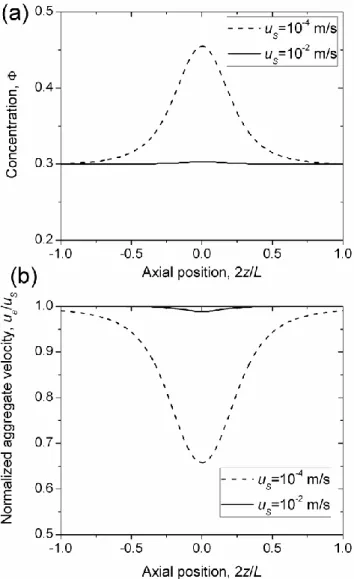
The theoretical steady-state dependencies of the particle concentration, , and of the aggregate speed, ua, on the position z along the tube are shown, respectively, in Figs. 2a and
2b for an applied external field, Hmax=100 kA/m and for two imposed speeds, uS=10-4 and 10-2
m/s. The flow is along the z-axis from the left to the right of the figures. At both extremities of the tube (z L/ 2), the particle concentration is equal to the initial volume fraction of the suspension, 0=0.3, as imposed in the model [cf. Eq. (12)]. When moving away from the
extremities to the tube middle-length, the magnetic field increases along with the suspension yield stress and the wall interaction force. This increases magnetic cohesion between particles, and therefore, wall interactions slow down the aggregates and increase their concentration according to the particle flux conservation. Therefore, the aggregate velocity profile exhibits a minimum [Fig. 2b] and the concentration profile shows a maximum [Fig. 2a], both at the tube middle-length (z=0) where the magnetic field is maximal. At an increasing imposed speed, uS, the aggregates pass faster through the tube and have less time to
get concentrated inside. Thus, both profiles become more homogeneous with the growing speed [cf. Figs. 2a, b]. In more details, as the flow speed increases, the relative importance of the magnetic contribution to the aggregate speed [second term on the right-hand side of Eq.
13
(11b)] decreases, and the latter (ua) approaches the suspension speed, uS, at high flow rates.
Note also that both ua(z) and (z)-dependencies are symmetric with respect to the tube middle
length (z=0). This is because the magnetic force term, 0MdH dz/ , responsible for an eventual asymmetry, appears to be negligible as compared to the wall interaction term, 2Y /R. It is worth mentioning that the situation is completely different for suspensions of nonmagnetic particles in a ferrofluid. These systems exhibit a weak yield stress and their behavior is dictated by the magnetic force, resulting in highly asymmetric concentration profiles in a similar geometry [Kuzhir et al. (2005)].
FIG. 2. Concentration profile (a) and aggregate velocity profile (b) along the tube axis for two different
suspension speeds, uS. The applied magnetic field is Hmax=100 kA/m. The origin of the z-axis is at the
middle-length of the tube, and the axial coordinate, z, is normalized by the half of the tube middle-length.
The theoretical concentration profiles, (z), allowed us to calculate the steady-state pressure-flow rate curves shown in Fig. 3 for the magnetic field Hmax=100 kA/m. As it is seen
in this figure, our model reproduces the expected behavior: an unstable decreasing branch of the P versus uS curve is followed by a stable increasing branch. For a better understanding of
14
the pressure difference, referred to as the hydrodynamic term and the yield stress term [the 1st and the 2nd terms on the right-hand side of Eq. (18)]. As already mentioned, with increasing suspension velocities, the particle concentration inside the tube decreases and approaches the initial volume fraction 0. Since the suspension yield stress is a growing function of the
particle concentration, the yield stress term, PY, decreases progressively with increasing
velocity attaining a high speed plateau with an asymptotic value,
/ 2 , 0 / 2 (2 / ) L , ( ) Y Y L P R B z dz
. On the other hand, the hydrodynamic term monotonically increases with the velocity. The sum of both contributions gives therefore the total pressure difference possessing a local minimum.FIG. 3. Theoretical dependency of the total pressure difference (solid curve) on the suspension speed at the
applied magnetic field, Hmax=100 kA/m. The two components of the pressure difference coming from the two
terms on the right-hand side of Eq. (18) are also shown. The calculations are performed for the following values of the free parameters: ra=10±1.0µm (aggregate radius) and c=0.29±0.02 (pre-factor in Eq. (10) for the yield
stress).
The theoretical pressure-flow rate curves are compared to the experimental ones in Fig. 4a for three different applied magnetic fields. In the experiments, the outlet flow rate fluctuated along with the pressure difference because of the suspension compressibility. These fluctuations were principally observed at the flow rates corresponding to the decreasing branch of P versus uS curve. Thus, for the unstable region of the experimental curves, P
stands for the time average of the pressure difference, P , introduced in Sec. II and uS
corresponds to the constant flow rate imposed by the piston motion, uS Qpiston/(R2), and is referred to as the imposed speed. The theoretical curves were obtained by fitting Eq. (18) to the experimental points using a single set of adjustable parameters, ra=10±1.0 µm and
c=0.29±0.02, for all the three curves. As it is seen in Fig. 4a, the theory qualitatively
reproduces the shape of the experimental curves and fits the experimental results reasonably well at low speeds, uS < 10-3 m/s, even though this comparison is delicate for unstable flows.
At higher speeds, the theory overestimates the pressure difference and this is probably because it does not take into account aggregate destruction by shear forces.
15 FIG. 4. Comparison between theoretical and experimental pressure-flow rate curves for different applied
magnetic fields (a). Theoretical predictions in the two opposite limits of low and high speeds are shown in figure (b) along with the experimental points at Hmax=100 kA/m.
To check this hypothesis, we inspect the suspension behavior in the opposite limit of high speeds, at which the aggregates do not span the tube diameter and their length decreases progressively with an increasing wall shear rate. This regime studied in details by Shulman and Kordonsky (1982) and Kuzhir et al. (2003) is characterized by the following pressure-speed relation:
/ 2 0 2 / 2 8 8 , ( ) 3 L p S D L u P B z dz R R
(19)Here, the suspension dynamic yield stress, D, comes from the hydrodynamic
dissipation generated by the aggregates and can be estimated by Eq. (10). The plastic viscosity p is usually field-independent and can be calculated using the Krieger-Dougherty
relation for a hard sphere suspension [Larson (1999)]: 2.5 max
0(1 0/ max) p
, with max 0.64
16
suspension speeds, the particle concentration is again assumed to be homogeneous along the tube and equal to the initial volume fraction 0. Both theoretical pressure-speed relations for
the two opposite speed limits are plotted in Fig. 4b along with the experimental curve, all three for the applied magnetic field Hmax=100 kA/m. As expected, the theory gives lower
values of the pressure difference at the high speed limit. At intermediate speeds, experimental points are situated between both theoretical limits pointing out to a possible transition between both regimes.
Another possible reason for the discrepancy between theory and experiments is connected to an increase of the aggregate thickness with the growing flow rate [cf. Assumption #2, Sec. III]. In theory, thicker clusters would lower the hydraulic resistance, K, of the aggregate network, which could reduce the slope of the pressure versus velocity curve. However, this scenario seems to be if not impossible, at least less likely because the dipole-dipole repulsion and lubrication between the aggregates should hinder their growth under the applied flow rate.
To inspect the effect of the applied magnetic field on the suspension flow, we plot in Figs. 5a and 5b the field dependencies of the critical pressure difference and suspension velocity corresponding to the minima of the pressure-flow rate curves. These figures demonstrate a good quantitative correspondence between experiments and theory for the critical pressure difference, Pc, and a qualitative correspondence for the critical suspension
velocity, uc, – both quantities show a monotonic increase with the applied field. As the
magnetic field increases, the suspension yield stress (and, consequently, the wall interaction force) becomes more important. This increases the total pressure difference and shifts the high-velocity plateau (of the yield stress term, PY,, cf. Fig. 3) and the pressure minimum to higher speeds resulting in an increasing field dependency of uc.
17 FIG. 5. Theoretical and experimental field dependencies of the critical pressure difference, Pc (a) and the
critical suspension speed, uc (b) corresponding to the minimum of the pressure-flow rate curves. In addition to it,
a theoretical dependency of the pressure difference, P0, at zero suspension speed is shown in figure (a).
Another important quantity emerging from the pressure-speed relations is the pressure difference, P0, at zero suspension speed. In theory, this pressure difference is developed in
an infinitely slow flow, which favors a nearly close packing of aggregates along the whole channel, so that the particle concentration at any location z is given by
max max a /(2 3) (2 / 9) 0.63
, with max being the maximum packing fraction of cylindrical aggregates. The value of P0 is calculated by integration of the yield stress
along the tube length: 0 / 2
max
/ 2(2 / ) L Y , ( ) L
P R B z dz
. The theoretical field dependency of the pressure difference P0 is represented by a dashed curve in Fig. 5a. The quantity P0appears to be roughly three times the critical pressure difference, Pc, in the considered range
of the magnetic fields, Hmax 0 150 kA/m. In our experiments, we were unable to achieve suspension speeds as slow as uS 10 m/s9 , at which the pressure-flow rate curve was expected to reach a low-speed plateau. Therefore, it was impossible to determine
18
experimental values of P0 by an extrapolation of the P versus uS curves to zero velocities.
These values could be measured in a pressure-controlled capillary rheometer.
B. Pressure/flow rate oscillations
As already stated, the pressure oscillations were principally observed in the range of flow speeds corresponding to the unstable branch of the pressure-flow rate curve. To inspect the waveforms of the pressure signal, we plot in Fig. 6 a-c the experimental time dependencies of the pressure difference P measured for the same applied magnetic field, Hmax=122 kA/m, and at imposed speeds, uS Qpiston/(R2), equal to 10
-4, 1.5∙10-4
and 8∙10-4 m/s, respectively. As it can be seen from the first two figures, the pressure oscillations are not perfectly regular. However, they have a well defined fundamental frequency and the shape reminiscent for a stick-slip motion of the suspension – a slow quasi-linear increase (stick) is followed by a drastic release of the pressure (slip). Their amplitude reaches 20% of the time average of the pressure difference, P , and decreases progressively with the imposed speed (as will be discussed below in more details), so that they completely disappear and are never observed at speeds corresponding to the stable increasing branch of the pressure-flow rate curve (case of Fig. 6c). Once appeared, the pressure oscillations are maintained during at least five hours, preserving their saw-tooth-like shape, as it is demonstrated in Fig. 6d for a magnetic field Hmax=52.5 kA/m and an imposed speed uS=3.1∙10-5 m/s.
19 FIG. 6. Temporal evolution of the pressure difference for the applied magnetic field Hmax=122 kA/m and for
imposed speeds, uS,=10-4 m/s (a), 1.5∙10-4 m/s (b) and 8∙10-4 m/s (c). A pressure signal recorded for a five hour
experiment at Hmax=52.5 kA/m and uS=3.1∙10-5 m/s is shown in figure (d). The initial plateau with P ≈ 0 in figs.
(a)-(c) corresponds to the flow in the absence of magnetic field, and a sharp increase of the pressure difference at the end of this plateau corresponds to the moment when the field is switched on.
Note that similar modulated oscillations have been predicted numerically by Bashkirtseva et al. (2009) for an unsteady shear rate response of repulsive concentrated
20
colloids subjected to a constant applied shear stress. These suspensions exhibited a non-monotonic shear rate versus stress dependency governed by the interplay between the electrostatic repulsion and solid friction between particles. In our case, the pressure oscillations are induced by magnetic interactions and illustrate another example supporting the statement that the instability has the same macroscopic origin for various systems – negative differential viscosity – whatever the interparticle interactions are.
At the unsteady-state regime, the outlet flow rate oscillated together with the pressure difference when a constant flow rate, Qpiston, was imposed by the piston. We inspect these
oscillations in Fig. 7a where the instantaneous flow rate, Qoutlet, and the instantaneous pressure
difference, P, both measured simultaneously, are plotted against the elapsed time for the
applied magnetic field, Hmax=122 kA/m, and the imposed speed, uS=Qpiston/(R2)=1.25∙10-4
m/s. As inferred from this figure, the suspension flow at the tube outlet has an intermittent character with a periodicity similar to that of pressure oscillations. As the pressure difference increases, the suspension does not flow out of the tube (Qoutlet=0), while when it decreases, a
rapid outflow is observed during a short period of time. Such a behavior can be attributed to the interplay between the blockage of aggregates and the suspension compressibility. This mechanism will be explained in more details at the end of this section in conjunction with the results of the structure observation. A more careful inspection of Fig. 7a shows that the outflow starts a little before the moment when the pressure difference achieves its maximum. This could be attributed to relaxation of particle structures leading to their retarded response to the varying flow rate. A dashed horizontal line in Fig. 7a corresponds to the constant imposed flow rate, Qpiston.
21 FIG. 7. Simultaneous temporal evolution of the pressure difference and the outlet flow rate (a), recorded at an
applied magnetic field, Hmax=122 kA/m, and an imposed speed, uS=1.25∙10-4 m/s. In figure (b), the dependency
of the instantaneous pressure difference, P(t), on the instantaneous flow rate, Qoutlet(t) is shown for the
pressure/flow rate oscillations shown in figure (a). The inset of figure (a) shows a drop of the MR suspension emerging from the tube outlet. The volume of the drop and the outlet flow rate were determined by image processing [cf. Sec. II]. A curvilinear shape of the drop is explained by the competition between the gravity and the magnetic forces. Note that the magnetic field at the tube outlet is about four percent of the maximum field at the tube middle length. The inset of figure (b) shows schematically a hysteresis cycle of the pressure-flow rate curve along with the pressure jump, Physt, and the flow rate jump, Qhyst.
An unsteady response of the suspension to a constant applied piston speed can also be analyzed with the help of the dependency of the instantaneous pressure difference, P(t), on
the instantaneous outlet flow rate, Qoutlet(t), shown in Fig. 7b for the same set of experimental
parameters. For convenience, we plot in the same figure the pressure-flow rate curve,
( piston)
P f Q
, measured for the same magnetic field. An experimental point of the P
versus Qpiston curve, for which the pressure-flow rate cycle is plotted, is marked by a text
22
vertical part of the cycle corresponds to a slow increase of the pressure difference at zero outlet flow rate. The upper quasi-plateau stands for an abrupt increase of the flow rate near the maximum pressure difference. We note that the oscillation cycle does not coincide with the hysteresis cycle of the pressure-flow rate curve [presented schematically in the inset of Fig. 7b], contrarily to what has been suggested by Quemada (1982) and Hatzikiriakos and Dealy (1992). In particular, the amplitudes of pressure and flow rate oscillations are somewhat lower than those, Physt and Qhyst, imposed by the hysteresis. Such inconsistency can be explained
by a relaxation of particle structures. A similar non-coincidence of the transient and steady-state pressure-flow rate curves has been revealed by Georgiou and Crochet (1994) in numerical simulations of compressible slit flows of polymer melts.
Since the fluid compressibility seems to be a necessary condition for the flow rate oscillations, the period of oscillations can be strongly influenced by the compression modulus and the total volume of the suspension. These effects could be inspected with the help of an equation relating the pressure and flow rate oscillations to the fluid compressibility. This equation, derived in Appendix, follows from the mass conservation law and takes the following form: 0 ( ) ( ) b piston outlet d P V Q Q t dt , (20)
where is the suspension compressibility and Vb0 is the suspension volume in the barrel.
Firstly, this equation, integrated over the oscillation period, T, allows us to check if the average outlet flow rate is equal to the imposed flow rate:
(1/ ) t T ( )
outlet outlet piston t
Q T
Q t dtQ . In experiments, the value Qoutlet appears to be slightly lower (by about 10%) than Qpiston. Such a discrepancy could come from some imprecision ofthe measurements of the outlet flow rate by image processing of the suspension drops emerging from the tube [cf. Sec. II and inset in Fig. 7a].
Secondly, Eq. (20) describes a linear increase of the pressure difference during the stick period (at Qoutlet≈0) and gives the following expression for the stick duration:
0( max min) b stick piston V P P t Q , (21)
where Pmax and Pmin stand for the maximum and minimum pressure differences during
oscillations.
This equation shows that the stick duration is inversely proportional to Qpiston and
varies linearly with Vb0, and thus depends on the piston position in the barrel [cf. Fig. 1]. To
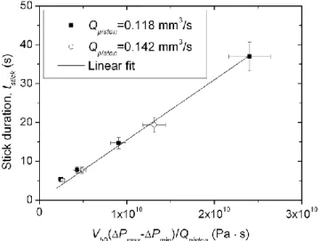
check this point we conducted a set of measurements at different initial piston positions and different piston speeds. The results of these measurements are shown in Fig. 8 as a dependency of the stick duration, tstick, on the factor Vb0(Pmax Pmin) /Qpiston. According to
23
the prediction of Eq. (21), all data points gather along a single line with a slope equal to 10 1
1.4 10 Pa
, as determined by a linear fit. This value appears to be quite close to the compressibility of silicon oil, 10 1
1.1 10 Pa
, reported in the literature [Kiyama et al. (1953)]. Since the flow oscillations depend on the initial piston position, we took care to perform all the measurements reported above at approximately the same value of Vb0 keeping
in mind that the piston position varied negligibly during a single run of the pressure versus time measurements.
FIG. 8. Dependency of the stick duration on the factor Vb0(Pmax Pmin) /Qpiston at different imposed flow
rates, Qpiston, and different initial positions of the piston in the barrel, corresponding to a suspension volume in
the barrel, Vb0, equal to 5.0, 6.7, 11 and 17 cm3. All the experiments were carried out at an applied magnetic field
of Hmax=122 kA/m.
We also checked that the stick duration (as well as the period of oscillations) depended on the suspension compressibility . For this purpose we conducted a supplementary measurement for the MR suspension gasified by air bubbling during one minute at vigorous stirring. The compressibility of such a suspension was estimated to be 3∙10-10
Pa and the stick duration appeared to be about two times longer than the one for the degasified suspension with 1.4 10 10Pa1. This comparison confirms the validity of Eq. (21) and proves that the suspension compressibility is one of the mechanisms governing self-exciting flow oscillations.
Note that at low enough imposed speeds, uS<0.5uc, the stick period is much longer
than the slip period, so that the oscillation period, T tstick, can be safely estimated by Eq.(21). According to this equation, at fixed values of and Vb0, the oscillation period is
proportional to (Pmax Pmin) /uS, so it depends, among other things, on the oscillation amplitude. The dependencies of these both quantities on the imposed speed are shown in Figs. 9a and 9b for different applied magnetic fields. In spite of some dispersion, the data follow a common decreasing trend. In particular, the pressure amplitude, (Pmax Pmin) / 2, seems to decrease with the speed and increase with the applied field [Fig. 9a]. Such a tendency may be
24
explained by the fact that, at increasing speeds, the aggregates spend less time inside the tube and probably form a sparser network resulting in smoother pressure variations. On the other hand, an increasing magnetic field causes a stronger blockage of aggregates likely leading to more intense oscillations. In what concerns the oscillation period, it also increases with the magnetic field and experiences a more pronounce decrease with the speed according to the following relationship: T ( Pmax Pmin) /uS. It is worth mentioning that the oscillations seemed to disappear (or, at least, were undetectable) at speeds somewhat lower than the critical velocity, uc, corresponding to the minimum of the pressure-speed curve. Perhaps, at
the speeds close to uc, the pressure amplitude was lower than the detection limit of our
pressure transducer.
FIG. 9. Dependencies of the pressure amplitude (a) and the oscillation period (b) on the imposed speed at
different applied magnetic fields. Solid curves correspond to eye-guidelines.
For a better understanding of the microscopic origin of the flow instability, we realized a flow of a dilute MR suspension (at a particle volume fraction 0=0.05) through a
transparent tube. The pressure signal, measured at Hmax=188 kA/m and uS=0.52 m/s, is shown
in Fig. 10 along with the snapshots of the suspension structure taken at different moments along the pressure versus time curve. Firstly, we distinguish column-like aggregates spanning
25
the tube diameter and occupying all visible tube volume. Second, the aggregates are more closely spaced in the region of high magnetic field in the vicinity of the pole pieces and are more sparsely spaced on the periphery. Such a distribution qualitatively corresponds to the theoretical concentration profile shown in Fig. 2a. Thirdly, when the pressure difference increases, the aggregates do not move and the structure seems to be frozen, as can be seen by comparing the snapshots A and B. However, a slow filtration of the suspending liquid through the network of aggregates was detected by motion of nonmagnetic impurities. Finally, once the pressure maximum is overcome, most of the aggregates detach from the tube wall and move rapidly towards the outlet as inferred from the snapshots C and D. When the pressure difference approaches the minimum, the flow is progressively decelerated and stops a few moments after the pressure difference starts to increase.
FIG. 10. Visualization of moving structures of a dilute (=0.05) MR suspension in a transparent tube. The snapshots were taken along the pressure versus time curve shown on the top of the figure. An enlarged view of the lower part of the tube is presented on the bottom of each snapshot and allows one to see stagnation of aggregates during the stick period (A and B) followed by a relatively intense motion of aggregates during the slip period (C and D)
Note that the same qualitative behavior is expected for more concentrated suspensions. Eventual quantitative difference may appear due to the fact that, with increasing particle concentration, the particle aggregates become thicker, as inferred from the visualization experiments of Grasselli et al. (1994). This may affect the hydraulic permeability of the structure [cf. Eq. (7)] and may therefore change the critical suspension speed along with the amplitude and period of oscillations.
26
In summary, these observations confirm that the stick-rupture events govern the unsteady flow of the suspension – the key hypothesis introduced at the beginning of the paper [Sec. I]. As already stated, the aggregates get blocked and ruptured from the walls when the hydrodynamic drag force is lower than a threshold value of the wall interaction force [cf. Eq.(11a)]. Since stick and rupture occur at different local speeds and pressures, two distinct threshold values of the wall force are apparently required. The upper limit corresponds to the onset of the slip and the lower limit corresponds to the blockage. The difference between both limits could have different nature. On the one hand, it could come from the difference between the static and dynamic yield stress, sometimes encountered in magnetorheology [Volkova (1998)]. On the other hand, it may appear as a result of the difference in local particle concentrations during the stick and the slip periods. Higher local speeds during the slip period would result in a lower concentration/yield stress, while quasi-zero speeds during the stick would cause a higher concentration/yield stress, as suggested by calculations of the concentration profiles [cf. Fig. 2a]. Whatever the mechanism is, we suggest the following suspension behavior in an unsteady flow. During the stick period, the pressure difference induces an extremely slow (almost undetectable) filtration flow of the suspending liquid through the particle structures. As the pressure difference increases, filtration becomes more intense, and the drag force increases until it overcomes the upper threshold of the wall force. Then, the aggregates will be ruptured from walls and the flow will start. The rupture event is likely accompanied by a decrease of the suspension hydraulic resistance due to either the replacement of the dense structures by the sparse ones or the appearance of lubrication gaps between the moving structures and walls. A decreasing hydraulic resistance will cause, at the beginning, fluid expansion and flow acceleration. During time, the particle structures will again be slowed down in the region of high magnetic field until the wall interaction force reaches the lower threshold, at which the structures will stick to the wall. The suspension compressibility results in a variation of the suspension speed in the tube, and the latter affects the instantaneous concentration profiles and the pressure difference.
As mentioned in the Introduction, similar pressure/flow rate oscillations have been discovered in capillary flows of polymer melts. In both cases, the flow instabilities come from wall interactions. However, the nature of these interactions is quite different. In the case of polymers, we deal with a pressure-dependent adhesion force of the molecules to the wall. In our case, the wall interaction likely originates from the shear magnetic force between the particle layers adjacent to the walls. Such an interaction is appropriate for relatively rough surfaces that can block small particles in the wall rugosities. In the case of a smooth wall surface (like the one of the polyvynil tube used in the visualization experiments), magnetic interactions between particles may dominate over their adhesion to the wall. The aggregates are expected to slide along the wall with a solid friction and without loss of entrapped particles. Being proportional to normal Maxwell magnetic stress, the friction force will also depend on the applied field and may conduct to phenomena similar to those observed for rough channels. Anyway, the role of the wall roughness should be carefully checked in further experiments.