HAL Id: hal-00432798
https://hal.archives-ouvertes.fr/hal-00432798
Submitted on 3 Dec 2009
HAL is a multi-disciplinary open access
archive for the deposit and dissemination of
sci-entific research documents, whether they are
pub-lished or not. The documents may come from
teaching and research institutions in France or
abroad, or from public or private research centers.
L’archive ouverte pluridisciplinaire HAL, est
destinée au dépôt et à la diffusion de documents
scientifiques de niveau recherche, publiés ou non,
émanant des établissements d’enseignement et de
recherche français ou étrangers, des laboratoires
publics ou privés.
Coupling and Level Repulsion in the Localized Regime:
From Isolated to Quasiextended Modes
K. Bliokh, Y. Bliokh, V. Freilikher, Azriel Genack, Patrick Sebbah
To cite this version:
K. Bliokh, Y. Bliokh, V. Freilikher, Azriel Genack, Patrick Sebbah. Coupling and Level Repulsion in
the Localized Regime: From Isolated to Quasiextended Modes. Physical Review Letters, American
Physical Society, 2008, 101 (13), pp.133901. �10.1103/PhysRevLett.101.133901�. �hal-00432798�
Quasi-Extended Modes
K.Y. Bliokh,1, 2 Y.P. Bliokh,3 V. Freilikher,4 A.Z. Genack,5 and P. Sebbah6
1Nonlinear Physics Centre, Research School of Physical Sciences and Engineering,
Australian National University, Canberra ACT 0200, Australia
2Institute of Radio Astronomy, 4 Krasnoznamyonnaya st., Kharkov 61002, Ukraine 3Department of Physics, Technion-Israel Institute of Technology, Haifa, 32000, Israel
4Department of Physics, Bar-Ilan University, Ramat-Gan, 52900, Israel
5Department of Physics, Queens College of the City University of New York, Flushing, New York 11367 6Laboratoire de Physique de la Mati`ere Condens´ee,
CNRS UMR6622 and Universit´e de Nice - Sophia Antipolis, Parc Valrose, 06108, Nice Cedex 02, France
The interaction of localized states in an open 1D random system is studied experimentally and the-oretically by manipulating their frequencies with changes in the internal structure of the sample. As the frequencies of two states come close, they are transformed into multiply-peaked quasi-extended modes. Level repulsion is observed experimentally and explained in terms of a model of coupled resonators. The spectral and spacial evolution of the coupled modes is described in terms of the coupling coefficient and Q-factors of resonators.
PACS numbers: 42.25.Dd, 78.70.Gq, 78.90.+t
Transport in open disordered media can be diffusive or localized, depending on the nature of the underlying quasimodes, which are, respectively, spread throughout the sample or exponentially peaked at random points, with a typical size given by the localization length [1–3]. The spatial overlap of localized modes which are close in frequency, couples these states and leads to the forma-tion of a series of exponential peaks known as necklace states [4–8]. These states are short-lived with broadened spectral lines [7, 9] and contribute substantially to the overall transmission in samples much thicker than the lo-calization length, L À lloc[6, 8]. Though such hybridized states are critically important in transport and may play an important role in the localization transition, their for-mation and the correlation between spatial and spectral properties has not been explored.
In this Letter, we study the transformation of localized states in a random sample as its configuration is altered and the coupling and hybridization of modes take place. Although level repulsion is ordinarily attributed to the diffusive regime [10, 11], the energy level correlation and repulsion in electron 1D localized systems has been found theoretically and numerically [12, 13]. Here we present the first experimental evidence of the level repulsion of the localized electromagnetic excitations. A simple the-oretical model is introduced which explains the spectral and spatial characteristics of coupled modes in terms of the loss and the coupling strength.
The experiment involves a rectangular microwave waveguide opened at both ends, which supports only a single transverse mode [8]. The waveguide is filled with a sample comprised of five 4 mm-thick blocks each of low and high indices of refraction randomly mixed with 31 randomly oriented 8 mm-thick binary blocks with low and high index halves. The field inside the sample is
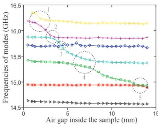
FIG. 1: (Color online.) Resonant frequencies of excited local-ized modes vs. the driving parameter - the air gap inside the sample. Five pair-interaction regions are circled.
weakly coupled to a cable which is translated along a 2-mm-wide slot cut along the waveguide in 1 mm steps. A sliding copper plate is pressed over the slot to eliminate leakage through the top of the waveguide. Field spectra are measured using a vector network analyzer.
Measurements are made in a sequence of configura-tions in which the spacing between two segments of the sample at a depth of 60 mm is increased in steps of 0.5 mm up to a maximum thickness of 14 mm. The spacing increment is sufficiently small to allow the identification of corresponding modes in configurations with different spacings. The position at which the air gap is introduced was chosen to correspond to the peak of a single local-ized mode. This allowed us to manipulate the frequency of the selected mode in the range from 14.5 to 16.5 GHz, which covers most of the band gap in the associated peri-odic sample. This is reminiscent of the tuning of a defect states through a band gap in a periodic structure as the
2
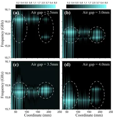
FIG. 2: (Color online.) Experimentally measured normalized wave intensity vs. frequency and coordinate inside the sample for two localized modes corresponding to region 2 in Fig. 1 at different values of the driving parameter. Excitations corre-sponding to the two effective resonators are circled.
defect width is increased up to a half-wavelength thick-ness. The mode frequency shifts across the frequencies of other localized states which makes it possible to study the coupling of two modes. We have also verified numer-ically that by changing the air spacing at other points in the sample at which other modes are peaked, it is pos-sible to couple several localized modes, thereby creating necklace states extended throughout the sample.
The spectral positions of the localized states as func-tions of the air gap introduced into the sample are plotted in Fig. 1. The frequencies of modes may cross or exhibit an anti-crossing. In the latter case (regions 1,2,4,5 of Fig. 1), the coupling within the sample is accompanied by an exchange of shape, as is seen in Fig. 2. When the frequencies of the modes are closest, the two localized states couple into double peaked quasi-extended modes with the same spatial intensity distribution, Fig. 2b and c. In contrast, region 3 in Fig. 1 shows a mode cross-ing in which the shapes are not exchanged. This is seen in Fig. 3 which shows the driven mode passing through the broad mode closest to the input. The two modes remain practically independent of each other, except for the low-intensity zone (dark horizontal line in Fig. 3) at the input mode which traces the destructive interference with the driven state.
Resonant wave transmission through an isolated local-ized state in a random sample can be described by a simple model of a wave tunneling through a resonator
FIG. 3: (Color online.) The same as in Fig. 2 for interaction region 3 in Fig. 1.
with semitransparent walls [2, 14, 15]. Dynamics of the field in the resonator obeys the oscillator equation with an external force and damping, which accounts for the incident wave and the finite Q-factor of the resonator, respectively [15, 16]. Extending this model to the case of
N localized states which are close in frequency, we arrive
at a system of N coupled oscillators with the external force acting on the first of these:
ψ00 1+ Q−11 ψ01+ (1 − ∆1)2ψ1= q1 2ψ2+ f0e−iντ , ... ψ00 l + Q−1l ψ0l+ (1 − ∆l)2ψl= ql l+1ψl+1+ ql l−1ψl−1, ... ψ00 N+ Q−1N ψN0 + (1 − ∆N)2ψN = qN N −1ψN −1 . (1) Here ψi(τ ) is the field in the ith resonator, τ = ω0t
is the dimensionless time (ω0 is a characteristic central
frequency of the problem), 1 − ∆i (|∆i| ¿ 1) is the di-mensionless eigenfrequency of ith resonator, Qi À 1 is the Q-factor describing the losses of the energy in the ith resonator, qi i+1 = qi+1 i ¿ 1 is the coupling coefficient of ith and (i + 1)th resonators due to the spatial overlap of their modes; f0 and ν, (|ν − 1| ¿ 1) are the
ampli-tude and frequency of the external field exciting the first resonator. The Q-factors can be written as [16]:
Q−1i = Γi (1 < i < N ) , Q−11,N = Γ1,N+
vgTin,out 2lω0 , (2)
where Γi is the dissipation rate in the ith resonator,
Tin,out are the transmission coefficient of the input and output of the system, vgis the wave group velocity inside
FIG. 4: (Color online.) Field amplitudes |A1,2|2(6) in the two
resonators as functions of the incident field frequency ν and detuning ∆ between the resonators. The underlying frequen-cies δν±
res (7) are depicted by the dashed lines. Parameters
are: f0= 1, q = 0.2, and Q−1= 0.1 (Q−1< q regime).
the resonator cavity, and l is the cavity length. The last term in Eqs. (2) accounts for the energy leakage through the outermost resonators [15, 16].
To establish the correspondence between the model (1) and localized states in a random sample, we assume, fol-lowing [14, 15], that ψi represents the peak field of ith localized state, qi i+1ψi is the amplitude of the field pen-etrating into the adjacent cavity, and f0is the amplitude
of the incident wave, ψ0, penetrating into the first
local-ization cavity. Since the locallocal-ization length is the only disorder-induced spatial scale in the problem, we have
qi i+1 ' exp (−di i+1/lloc) , f0' ψ0exp (−din/lloc) ,
Tin,out ' exp (−2din,out/lloc) , l ∼ lloc . (3) Here di i+1 = |Xi+1− Xi| is the distance between adja-cent states at coordinates Xi+1 and Xi, whereas din =
X1 and dout= L − XN are the distances from the edge localized states to the corresponding ends of the sam-ple. Deterministic equations (1)–(3) provide an effective description of coupled modes in 1D random system.
Substituting ψi= Aiexp ( −iντ ), the set of equations (1) is reduced to an algebraic equation ˆH ~Ψ = ~F with
ˆ H = C1 −q1,2 ... 0 0 −q1,2 ... −ql−1,l 0 0 ... −ql−1,l Cl −ql,l+1 ... 0 0 −ql,l+1 ... −qN −1,N 0 0 ... −qN −1,N CN , (4) ~ Ψ = (A1, ..., AN)T, and ~F = f0(1, 0, ..., 0)T, where Ci = (1 − ∆i)2− ν2− iνQ−1i ' 2 (1 − ∆i− ν) − iQ−1i . The homogeneous equation ˆH ~Ψ = 0 determines a set of independent eigenmodes of the system, with eigenfre-quencies being the eigenvalues of the matrix (4).
For the sake of simplicity, we consider the case of two interacting modes, N = 2, and assume that Q1 = Q2 ≡
FIG. 5: (Color online.) The same as in Fig. 4 for the param-eters q = 0.2 and Q−1= 0.25 (Q−1> q regime).
Q and q1 2≡ q. Then, the complex eigenfrequencies ν± =
1 + δν± are given by δν± = −∆1+ ∆2 2 − i Q−1 2 ± 1 2 p (∆1− ∆2)2+ q2, (5)
This equation describes anti-crossing of levels (level re-pulsion) which occurs at finite q 6= 0, when the modes of isolated resonators couple into collective eigenmodes. The minimal frequency gap q is achieved at resonance, ∆1= ∆2. Away from the resonance, |∆1− ∆2| À q, the
eigenmodes tend to the modes of isolated resonators, ex-changing when passing through the resonance, i.e., + (−) eigenmode corresponds to the first (second) resonator at ∆1¿ ∆2 and to the second (first) one when ∆1À ∆2.
It is important to note that the level repulsion of elec-tromagnetic modes takes place in the regime of strong localization, cf. [13].
If the system is excited by an incident monochromatic wave with the real frequency ν = 1 + δν, as it is in the experiment, the complex amplitudes A1,2in the two
res-onators can be obtained from ˆH ~Ψ = ~F , which yields A1 = − £ 2 (∆2+ δν) + iQ−12 ¤ f0 D , A2= qf0 D , (6) D = £2 (∆1+ δν) + iQ−11 ¤ £ 2 (∆2+ δν) + iQ−12 ¤ − q2
Behavior of |A1,2|2 is essentially determined by the
de-nominator |D|2, which is minimal at frequencies
δνres± = − (∆1+ ∆2) 2 ± 1 2Re p (∆1− ∆2)2+ q2− Q−2. (7) The amplitudes A1,2 and frequencies δνres± characterize
resonant excitation of the system by an external source. Note that Eq. (7) coincide with Eq. (5) only in the lossless case Q−1 = 0. Otherwise, there are two dif-ferent regimes of the excitation of coupled resonators, determined by the ratio between losses Q−1 and cou-pling q. If losses are small, Q−1 < q, two branches δν±
res
4
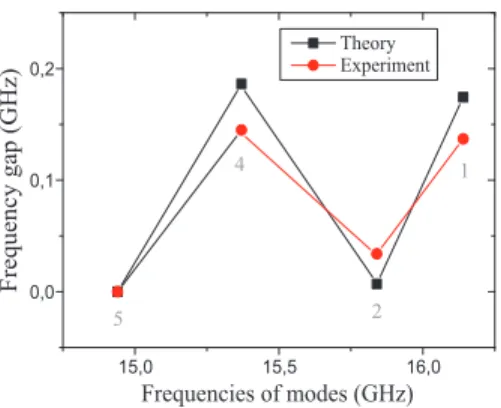
FIG. 6: (Color online.) Experimentally measured and theo-retically calculated (Repq2− Q−2) minimal frequency gaps
for pairs of interacting modes 1,2,4,5 presented in Fig. 1.
gap pq2− Q−2, Fig. 4. If losses prevail over the cou-pling, so that Q−1> q, the frequencies δν± merge in the interaction region (∆1− ∆2)2≤ |q2− Q−2|, Fig. 5.
The amplitudes (6) as functions of the frequency ν and detuning (∆1− ∆2) are shown at Q−1< q and Q−1> q
in Figs. 4 and 5, in which the main features observed ex-perimentally are seen (different values of ∆ correspond to different frames of Figs. 2 and 3). To facilitate com-parison with the experimental Figs. 2 and 3, the second, output resonator is driven in Fig. 4 (∆1 ≡ 0, ∆2 ≡ ∆),
while the first resonator is driven in Fig. 5 (∆1 ≡ ∆,
∆2≡ 0)). In the regime Q−1< q, it is seen in Figs. 2 and
4 that in the interaction region (Figs 2b and c) fields in both resonators exhibit double-peaked spectra (level re-puslion). Collective excitation of two resonators signifies formation of a quasi-extended necklace state there. Re-markably, away from the resonance (Figs. 2a and d) the first resonator is effectively excited at one of the resonant frequencies, close to δν = −∆1, Fig. 4a) while the second
resonator is equally excited at both the resonant frequen-cies δν±
res' ∆1,2 (Fig. 4b). In the regime Q−1> q, both
Figs. 3 and 5 show that the second resonator is excited with a single-peak spectrum (Fig. 5b), while the first one exhibits two peaks separated by a dark area driven with the frequency of the second resonator (Fig. 5a) [17].
The measured and calculated values of the frequency gap between coupled modes are presented in Fig. 6. The parameters of the system are:
ω0
2π ' 15.5GHz, lloc' 12mm, ω0Γ ' 7 × 10
7s−1, (8) and vg' c/2.4, whereas positions of the localized modes interacting in the regions 1–5 (Fig. 1) equal, respectively:
X1 ' 64 : 64 : 7 : 64 : 64 mm ,
X2 ' 117 : 192 : 64 : 128 : 235 mm . (9)
Substituting values (8) and (9) into Eqs. (2) and (3) yields Q−1
1,2 and q. We calculated minimal frequency gap
for interacting pairs 1,2,4,5 (for which Q−11 ∼ Q−12 [17])
as Repq2− Q−2 with Q−1 = (Q−1
1 + Q−12 )/2, and
com-pared with the measured gap from Fig. 1. Fig. 6 shows good agreement between the experiment and model.
In conclusion, we have observed level repulsion in the localization regime and have shown that it reflects the coupling of localization centers. The occurrence of anti-crossing or anti-crossing of quasimodes as a sample configu-ration changes depends upon the ratio of the coupling strength between localized states and loss. These factors determine the statistics of nearest neighbor spacings and correlation in the widths of neighboring modes and thus the nature of wave propagation.
We thank B. Hu, J. Klosner, H. Rose, and Z. Oz-imkowski for suggestions regarding the construction and implementation of the waveguide assembly. This research was sponsored by the Linkage International Grant of the Australian Research Council, National Science Founda-tion (DMR-0538350), PSC-CUNY, the Centre NaFounda-tional de la Recherche Scientifique (PICS #2531 and PEPS07-20), and the Groupement de Recherches IMCODE.
[1] P.W. Anderson, Phys. Rev. 109, 1492 (1958).
[2] M.Y. Azbel, Solid State Commun. 45, 527 (1983); Phys. Rev. B 28, 4106 (1983).
[3] P. Sheng, Scattering and Localization of Classical Waves
in Random Media (World Scientific, Singapore, 1990).
[4] N.F. Mott, Phil. Mag. 22, 7 (1970).
[5] I.M. Lifshits, and V.Y. Kirpichenkov, Zh. Eksp. Teor. Fiz. 77, 989 (1979) [Sov. Phys. JETP 50, 499 (1979)]. [6] J.B. Pendry, J. Phys. C 20, 733 (1987); Adv. Phys. 43,
461 (1994).
[7] J. Bertolotti et al., Phys. Rev. Lett. 94, 113903 (2005); Phys. Rev. E 74, 035602 (2006).
[8] P. Sebbah et al., Phys. Rev. Lett. 96, 183902 (2006); J. Opt. Soc. Am. B, 24, A77 (2007).
[9] V. Milner and A.Z. Genack, Phys. Rev. Lett. 94, 073901 (2005).
[10] T. Guhr, A. Muller-Groeling, and H. Weidenmuller, Phys. Rep. 299, 190 (1998).
[11] Altshuler ???? What is the reference? (Question for Azi)
[12] L. Gor’kov,O. Dorokhov, F. Prigara, Sov. Phys. JETP 57, 838, (1983).
[13] A.V. Malyshev, V.A. Malyshev, and J. Knoester, Phys. Rev. Lett. 98, 087401 (2007).
[14] K.Y. Bliokh et al., J. Opt. Soc. Am. B, 21, 113 (2004); Phys. Rev. Lett. 97, 243904 (2006).
[15] K.Y. Bliokh et al., Rev. Mod. Phys. (2008, to be pub-lished); arXiv:0708.2653.
[16] Y.P. Bliokh, J. Felsteiner, and Y. Slutsker, Phys. Rev. Lett. 95, 165003 (2005).
[17] It should be noted that the experiment depicted in Fig. 3 does not exactly correspond to the model case of Fig. 5 because two localized modes of Fig. 3 have significantly different Q-factors, Q−1
1 À Q−12 . This diminishes the
in the complex plane. Nonetheless, our simplified model with Q1 = Q2 describes quantitatively all the main