HAL Id: hal-02951745
https://hal.archives-ouvertes.fr/hal-02951745
Submitted on 28 Sep 2020
HAL is a multi-disciplinary open access
archive for the deposit and dissemination of
sci-entific research documents, whether they are
pub-lished or not. The documents may come from
teaching and research institutions in France or
abroad, or from public or private research centers.
L’archive ouverte pluridisciplinaire HAL, est
destinée au dépôt et à la diffusion de documents
scientifiques de niveau recherche, publiés ou non,
émanant des établissements d’enseignement et de
recherche français ou étrangers, des laboratoires
publics ou privés.
A framework for managing the imperfect modularity of
variability implementations
Xhevahire Tërnava, Philippe Collet
To cite this version:
Xhevahire Tërnava, Philippe Collet.
A framework for managing the imperfect
modular-ity of variabilmodular-ity implementations.
Journal of Computer Languages, Elsevier, 2020, pp.1-39.
A Framework for Managing the Imperfect Modularity of Variability
Implementations
Xhevahire
Tërnava
a,∗,
Philippe
Collet
b aUniversité de Rennes 1, INRIA/IRISA, Rennes, France bUniversité Côte d’Azur, CNRS, I3S, Sophia Antipolis, FranceA R T I C L E I N F O Keywords:
Software product line engineering Variability management Variability implementation Imperfectly modular variability Domain specific language
A B S T R A C T
In many industrial settings, the common and varying features of related software-intensive sys-tems, as their reusable units, are likely to be implemented by a combined set of traditional tech-niques. Features do not align perfectly well with the used language constructs, e.g., classes, thus hindering the management of implemented variability. Herein, we provide a detailed framework to capture, model, and trace this imperfectly modular variability in terms of variation points with variants. We describe an implementation of this framework, as a domain-specific language, and report on its application on four subject systems and usage for variability management, showing its feasibility.
1. Introduction
Software product line(SPL) engineering is the common methodological process for developing together a set of related software-intensive systems. The process is intended to achieve mass customization with methodological reuse of the software systems seen as products, leading to lower cost and time-to-market and improved quality. At the domain level, the variability of considered systems is commonly described in terms of their common and varying features, as their reusable units, in a feature model (FM) [47,48,22]. Then, in a forward engineering approach, their features are realized in different software assets, including code assets. Consequently, the objective is that various systems can be systematically derived from a common and managed set of software assets.
Although variability is largely studied in the context of software product lines and product families [22], most modern software-intensive systems, being organized as a software product line or not, are variability-intensive [43,34]. In systems that are not part of a product line, that is, variability-rich systems, the implemented variability in their code assets is neither explicit nor documented. This is because the variability of code assets is typically realized by a diverse and combined set of traditional techniques, such as inheritance, design patterns, overloading, or generic types. However, their used code units, such as classes, or methods in object-oriented programming, do not align well with the domain features or, simply put, neither features nor variation points with variants (their definition is given inSection 2) are by-product of traditional techniques [20]. This hinders the management of the variability of code assets, which seems to be extensive in real variability-rich systems [17,89].
For example, let us consider the system of JavaGeom [57], an example of a real variability-rich system, which is not organized as a software product line but is variability-intensive, and was used in a previous study [89]. It is an open-source geometry library for Java that is easily understandable. Although not presented and organized as anSPL, it is architected around well-identified features. Compared to similar real variability-rich systems that are of over 100 K LoC and thousands of potential vp-s with variants [17,89], JavaGeom has over 35 K LoC, being a medium-size variability-rich system. InFigure 1is given an excerpt of its created feature model, which consists of five features. The abstract feature [90] JavaGeomFM does not require an implementation, it is used to represent conceptually the Jav-aGeom variability-rich system. As for the other four concrete features, StraightCurve2D, Line2D, Segment2D, and Ray2D, a form of their implementation is given inListing 1, using Java language. At first sight, the mapping between features inFigure 1and used code units, classes, inListing 1seems to be straightforward, but it is more complicated. First, the feature names and class names are mostly different, for instance, the feature name Line2D is different from its implementation class StraightLine2D. Besides, the classes extend or implement other classes and interfaces, show-ing more dependencies at the code level than that features have at the domain level. Then, the implemented variability by method overloading, distance() in lines 4-18, is not modeled in theFM. This single example, where only the
Figure 1: An excerpt of the feature model (FM) of JavaGeom variability-rich system (The FM is created using the FeatureIDE tool [62]).
1 /* Class level variation point, vp_AbsLine2D */
2 public abstract class AbstractLine2D extends
AbstractSmoothCurve2D implements
SmoothOrientedCurve2D, LinearElement2D {
↪ ↪ 3
4 /* Method level variation point,
vp_distance */
↪ 5
6 /* First variant of vp_distance */
7 public double distance(Point2D p) {
8 return distance(p.x(), p.y());
9 }
10
11 /* Second variant of vp_distance */
12 public double distance(double x, double y) {
↪
13 Point2D proj = projectedPoint(x, y);
14 if (contains(proj))
15 return proj.distance(x, y);
16 /* Omitted code */
17 return dist;
18 }
19 /* Omitted code */
20 }
21 /* First variant, v_Line2D, of vp_AbsLine2D */
22 public class StraightLine2D extends
AbstractLine2D implements SmoothContour2D,
Cloneable, CircleLine2D {
↪ ↪
23 /* Omitted code */
24 }
25 /* Second variant, v_Segment2D, of vp_AbsLine2D
*/
↪
26 public class LineSegment2D extends
AbstractLine2D implements Cloneable,
CirculinearElement2D {
↪ ↪
27 /* Omitted code */
28 }
29 /* Third variant, v_Ray2D, of vp_AbsLine2D */
30 public class Ray2D extends AbstractLine2D
implements Cloneable {
↪
31 /* Omitted code */
32 }
Listing 1:An excerpt of variability implementation in the JavaGeom variability-rich system considered as a software product line.
techniques of inheritance and overloading are used, shows some difficulties in mapping features at the code assets of a given variability-rich system. In real variability-rich systems, the problem is exacerbated as features are often not implemented by a single class or method. This is due partly to the many design choices that influence the usage of different implementation techniques to structure the variability implementations, and partly to the crosscutting nature of features with code units [51].
To overcome such variability management difficulties, existing approaches use annotations, often preprocessor directives [59], or have proposed to put into separate modules, for example, into aspects, feature modules, or delta modules [6], all lines of code that belong to each specific domain feature [7, 83]. In addition, different tools are proposed, for example, pure::variants [36], code tagging [42], or those that propose to use colors, at the representation layer of code, for distinguishing the lines of code that implement each feature [49]. Analysing which technique, tool, or combination of them [67] fits best to implement or manage some variability is hard to conclude as none of them is yet a preferred one [6], while theSPLapplication domains are themselves largely diverse. However, except for tool-based approaches, most of the proposed solutions affect the initial decomposition or design of code assets, such as their object-oriented design [7], and in case of migration from a variability-rich system to an SPL, a massive code refactoring is required. As a consequence, when an object-oriented design is refactored, for example, to a feature-oriented design [6], the logical relation among code units is usually lost at the code level. For instance, the alternative relation among the three child features inFigure 1may lose, which relation is realized by subclasses through the technique of inheritance inListing 1.
Facing these issues, our work takes the assumption that one can keep unchanged the initial design of code assets of a variability-rich system, that is, without the need to migrate it to anSPL, and manage its variability in terms of variation points with variants, as initial variability abstractions [45]. To the best of our knowledge, no variability management approach is currently addressing the early steps of capturing and modeling the variability of code assets of a variability-rich system [54,5,13,16,75,80], especially not when a subset of variability implementation techniques are used in combination [45,26].
Towards an approach that meets our assumption and goal on managing variability implementations in code assets of a variability-rich system, we proposed, in a previous work [88], a three step framework to manage such variability when a combined set of traditional techniques is used (Section 4). Such techniques expose a form of what we define as imperfectly modular variability (Section 3), as domain features do not perfectly align with the used code units. The framework is devised by analysing up to ten common variability implementation techniques used in variability-rich systems, which are revealed in a recent catalog of 21 traditional and emerging techniques [87] (cf.Section 2.2.3). This catalog is at first based on 7 previous frameworks, taxonomies, and catalogs [6,33,68,72,74,73,26]. For the purpose of our framework, we analysed the characteristics properties of these techniques, such as binding time.
1. The framework provides the means to make explicit the variability of code assets by capturing the used variability implementation techniques in terms of variation points (vp-s) with variants, as variability abstractions.
2. It then makes possible to use the captured vp-s with variants to model the variability of code assets in a frag-mented way into so-called technical variability models (Section 4.2.2). Towards this, five types ofvp-s are
identified and suggested for use, whereas what is a fragment aims at being flexible. It can be a package, file, or class with variability that worth to be modeled separately.
3. The framework also introduces the possibility to establish n-to-m trace links between the modeled variability of code assets and their respective features in some feature model at the domain level.
Herein, we extend this work in several aspects:
- First, we further detail the concept of imperfectly modular variability and determine its induced challenges (Section 3), which motivate the whole presented work.
- We present the three steps of our framework with all necessary details, formal definitions, and related illustrations (Section 4), mainly by using a running variability-rich system introduced inFigure 1andListing 1.
- We present the implementation of the framework as a small textual domain-specific language (DSL) in Scala, publicly available. Its technical foundations are also given inSection 5.
- We report on a series of experiments on the application of thisDSLto four subject systems (Section 6). This evaluation was conducted around four research questions to study the encountered implementation techniques, types of vp-s, the multiplicity of trace links, and to evaluate the overhead in modeling with theDSL.
- We also evaluate the capacity of usage of the proposed framework for variability management by adapting a previous work on early consistency checking [86] and showing how the tooled framework enables us to integrate such a checking method in one of the subject systems (Section 7).
Threats to the validity of the framework and its implementation are discussed inSection 8. We also put our con-tribution into perspective with some related work, including industrial approaches for managing variability at the implementation level (Section 9). Finally,Section 10concludes this article by summarizing the contributions and discussing future work.
2. Background
Some of the key aspects of the variability management of a system, being it organized as anSPLor not, is the ability to model the realized variability of code assets and then possibly to trace it to its specified variability. In the following, we provide a background on variability modeling, realization, and traceability.
2.1. Variability modeling
Since its first presentation byKang et al.[47], feature modeling has progressively been widely adopted as a means for scoping and modeling the variability of software systems within anSPLin terms of features [28]. A feature model
𝖼𝗑 𝗏𝖺 𝗏𝖻 𝗏𝖼 ...
a) 𝖼𝗑
𝗏𝖺 𝗏𝖻 𝗏𝖼 ...
b)
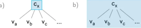
Figure 2: The variation point (vp) concept as: a) a variable point (i.e., the 𝖼𝗑), b) a variable part (i.e., the 𝖼𝗑 with
variants). The 𝖼𝗑is the common part for variants 𝗏𝖺, 𝗏𝖻, and 𝗏𝖼.
(FM) is a tree structure of features, consisting of mandatory, optional, or, and/or alternative logical relations between features with their cross-tree constraints, implies and/or excludes, that are expressed in propositional logic. InFigure 1 is given an example of anFM, for the JavaGeom variability-rich system. Its main feature, JavaGeomFM, represents conceptually the JavaGeom domain. It has a mandatory feature, StraightCurve2D, with three alternative features, Line2D, Segment2D, and Ray2D. While anFMcan have cross-tree constraints between features, there is none in this example. Semantically, anFMrepresents all the valid software systems (i.e., the feature configurations) within anSPL or within a variability-rich system.
2.2. Variability realization
We now provide some background on the variability of code assets, the variability modeling, and the used tech-niques for its realization in variability-rich systems.
2.2.1. Reusable code assets
In real variability-rich systems, despite the programming paradigm (e.g., object-oriented, or functional), the im-plementation of reusable code assets complies, mostly, to a commonality and variability approach [26]. Specifically, a domain is decomposed into subdomains then, within each subdomain, the commonality is factorized from the vari-ability. Thus, the code assets consist of three parts: the core, commonalities, and variabilities. The core part is what remains of the system in the absence of any particular feature [91], that is, the assets that are included in any software system. A commonality is a common part of the related variant parts within a subdomain. After the commonality is factorized from the variability and implemented, it becomes part of the core (i.e., it is buried in the core [26]), except when it represents some optional variability. On the other hand, the variant parts are used to distinguish the software systems in the domain. A subdomain can have more than one common and variant part. The core with the commonalities and variabilities of all subdomains constitute the wholeness of code assets in a variability-rich system.
2.2.2. Commonality and variability abstractions
While features are commonly used to model the domain variability of anSPLor variability-rich system (i.e., as problem-oriented abstractions), the commonalities and variabilities in code assets are usually abstracted in terms of variation points (vp-s) with variants, respectively (i.e., as solution-oriented abstractions for the realized variability of
code assets) [27,28,76]. Moreover, unlike features that are mere names, vp-s with variants are related to concrete elements in code assets. Originally, "a variation point identifies one or more locations at which the variation will occur" [45], whereas the way that a variation point is going to vary is expressed by its variants.
In the literature, there are few different understandings of a vp [85, pg. 16]. Mostly, a vp is recognized (i) as an abstraction of a location or point that varies in reusable code assets (cf. Figure 2a) [45], (ii) as a variable part (cf.Figure 2b) [9], or (iii) as an abstraction of a variability implementation technique [22, pg. 48]. But, these all have a common meaning. Specifically, the variable part is like an organizing container [9]. It contains the location where some variability happens in reusable code assets (i.e., the variation point), the variants, and the used technique to implement them. In this work we use the same meaning of vp-s with variants.
2.2.3. Variability implementation techniques
The used techniques for implementing variability in anSPLor variability-rich system are known as variability implementation techniques [32,87]. They came from several programming paradigms and are supported by different constructs in different programming languages, which in turn offer different properties for features or vp-s with vari-ants. Examples of such techniques are inheritance, preprocessor directives, feature modules, or some design patterns. For example, inListing 1is shown the usage of two variability implementation techniques, inheritance and overload-ing. They implement two variation points (see the comments inListing 1), lines 1-20 and lines 4-18, respectively,
which have different properties. Both of them have different granularity, of class and method levels, and during the product derivation, they will be resolved at different times, runtime and compile time, respectively.
Because of the large diversity of techniques, an important issue for variability implementation is the ability to evaluate and choose a technique that will fulfill best some given variability requirements. Therefore, for various tech-niques, several evaluation schemas have emerged, mainly from academia, in the form of frameworks, taxonomies, and catalogs. They all evaluate a different subset of techniques regarding different properties, some of which overlap. For instance,Svahnberg et al.[84] propose to group and evaluate techniques by 2 main properties, according to the size of software entities with variability or variable (components, frameworks, and lines of code), and their latest binding time. Then, the others provide some more concrete and enriched sets of techniques and evaluation properties. For instance,Patzke and Muthig[72] evaluate 8 techniques with up to 6 properties, Patzke and Muthig[73] evaluate 1 technique based on 10 properties,Muthig and Patzke[68] evaluate 8 techniques with up to 8 properties,Gacek and Anastasopoules[33] evaluate 7 techniques with up to 7 properties,Patzke et al.[74] evaluate 7 techniques with up to 14 properties, orApel et al.[6] evaluate 10 techniques with up to 15 properties.
A more systematic evaluation is provided by a recent catalog [87] that provides an updated set of 21 variability implementation techniques. They are categorized by their 24 different properties that they may support or belong to, such as the logical relation that a technique provides among variants of a vp, their granularity, binding time, traceability, language-based, tool-based, or in which programming paradigm it belongs to. As a main property, all 21 techniques are categorized into traditional or emerging techniques:
• Traditional techniques are those that have emerged and evolved separately and quite before the emergence of the SPLparadigm. They encompass methods that are used for single system development but provide the necessary mechanisms to be good candidates forSPLengineering. Although, using these techniques feature does not have a first-class representation in implementation. Such techniques are inheritance, overloading, or design patterns. For instance, the traditional technique of overloading provides an alternative logical relation between variants of a vp, but it cannot be used to provide an or or optional logical relation between them [33,72,87].
• Emerging techniques have appeared with theSPLengineering advances. Here, the concept of feature is a first-class citizen at the code level. Such techniques are frames [10], feature modules [6], or delta modules [78]. For instance, the emerging technique of feature modules provides good support for realizing the or logical relation between feature modules in code assets, but it hardly supports the realization of alternative or optional logical relation between them [6,87].
Instead of eliminating this diversity, for example, by proposing to implement the whole variability only at the class level, or by mixing two languages, such as the case of C with #ifdef-s, or proposing to use another code unit, such as feature module, that crosscuts with the prior design of code, in this work we strive to model the implemented variability of variability-rich systems by capturing and modeling different properties of vp-s with variants that are implemented by traditional techniques. Specifically, considering the scope of our study, we retain the ten object-oriented traditional techniques and software design patterns provided in the catalog, which are commonly used to implement variability-rich systems. The other techniques, such as preprocessors or feature modules; aim at a methodological development of related software systems as anSPL, therefore they are outside the scope of this study. This enables to aim at variability management in variability-rich systems implemented with such traditional techniques. Apart from this, inSection 4.1.2 we detail four characteristic properties of vp-s with variants that are essential for managing the variability in code assets, such as logical relation, binding time, evolution, and granularity. It is important to emphasize that, in principle, each vp is associated with a single variability implementation technique, whereas the same technique can be used to implement several vp-s within a variability-rich system.
2.3. Variability traceability
The CoEST1defines a trace (noun 2) as "a specified triple of elements comprising: a source artifact, a target
arti-fact, and a trace link associating the two artifacts", and the traceability as "the potential for the traces to be established and used" [23].
The concept of traceability is already used for different reasons in single software engineering, mostly to trace requirements. But, inSPLand variability-intensive systems engineering the relevant entities that are required to be traced and the semantics of trace links are different. Specifically, an explicit capturing of variability information and
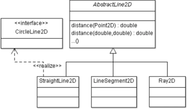
Figure 3: The detailed design of the given excerpt of JavaGeom variability-rich system inListing 1.
𝖲𝗍𝗋𝖺𝗂𝗀𝗁𝗍𝖢𝗎𝗋𝗏𝖾𝟤𝖣 ⟼ AbstractLine2D 𝖫𝗂𝗇𝖾𝟤𝖣 ⟼ StraightLine2D 𝖲𝖾𝗀𝗆𝖾𝗇𝗍𝟤𝖣 ⟼ LineSegment2D
𝖱𝖺𝗒𝟤𝖣 ⟼ Ray2D
Note: Along this work, the non-italic names stand for features, the italic names stand for code unit, whereas a prefix "vp_" and "v_" is used for variation points and variants. These prefixes are reintroduced inSection 4.1
Figure 4: The mapping of domain features inFigure 1to the code units inFigure 3. The ⟼ has the "implemented by" meaning.
their modeling of dependencies and relationships separate from other development artifacts is needed [16]. This is well known as variability traceability [4,5]. It includes the ability to trace the specified variability in problem space to the realized variability in solution space, for example, the ability to trace features inFigure 1, as source artifacts, to their respective vp-s with variants in implementation inListing 1, as target artifacts.
According to the generic traceability model [39], trace links are basically established to meet a specific usage purpose and need to be maintained during the whole engineering process [75]. Moreover, variability trace links can be established for different reasons and by different stakeholders [24,5]. For example, they can be used for (semi)automating different processes during the application engineering [75], namely for resolving the variability during product derivation, evolving, checking consistency, addressing, or comprehending variability. In this work, we focus on the ability to establish these variability trace links and use them for checking the consistency of variability. For example, after tracing features inFigure 1to their respective vp-s with variants inListing 1, trace links can be used to check whether each specified feature in theFMis addressed at the code level, or whether the alternative relation between three features, Line2D, Segment2D, and Ray2D, is properly considered during their implementation in code.
3. Imperfectly modular variability
Variability management would be simplified in case that each domain feature was implemented in a modular way, by a single language code unit [6], as the mapping of domain features to their implementation would be straightforward. But, this is clearly not the case in real variability-rich systems [89], with the current language constructs and design methods, where variability is implemented by using a combined set of traditional techniques, such as inheritance, overloading, generic types, or design patterns. These techniques do not enable us to completely align the domain features to the places where they are implemented, leading to what we define as imperfectly modular variability at the implementation level. On the contrary, a perfect alignment of a domain feature to its implementation would make traces trivial to be established.
To illustrate what imperfectly modular variability means, let us consider the given features inFigure 1 for Jav-aGeom variability-rich system and the excerpts of their respective implementation as inListing 1. Focusing on the implementation techniques inListing 1, the design of which is shown inFigure 3, the abstract class, AbstractLine2D, is a vp and its three subclasses, StraightLine2D, LineSegment2D, and Ray2D, represent its variants that are created by specializing its implementation. In this way, features in theFMinFigure 1 seem to have a direct and modular mapping in implementation, as is shown inFigure 4, where ⟼ has the implemented by meaning.
Actually, this perfect form of modularity hardly exists. The variation point AbstractLine2D and its variants have a lot of internal variabilities. For instance, the method distance() in AbstractLine2D is another vp with two alternative variants implemented using the technique of overloading (cf.Listing 1in lines 6-9 and 11-18). The variants of distance() can be considered as implementations in finer grained modules. They represent some technical and nested variability, which could be specified or not in theFM, but still need to be documented, traced, and managed (e.g., in order to be resolved). Then, the feature Line2D uses several vp-s, such as AbstractLine2D, CircleLine2D,
the variant StraightLine2D (cf.Figure 1andFigure 3), plus their finer grained vp-s mentioned just before. Imperfectmodularity comes from the fact that a feature is a domain concept and its refinement in code assets is a set of vp-s with variants, even if they are modular, meaning that it may not have a direct and single mapping. Also, while it would be preferable to use a single variability implementation technique to implement the variability of a system, none of the existing techniques is yet "a preferred one" [6], which could cover all kinds and properties of variability that may appear in different domains. In our illustrative example, the traditional techniques of inheritance and overloading are used together, which induces a class and method granularity of variability with runtime and compile time binding, respectively. In these techniques, the conceptual features do not have a first-class representation in implementation. Still, a degree of modularization of variability can be achieved when used with variability management or traceability in mind. Therefore, we propose the following definition.
Definition 1. An imperfectly modular variability in implementation occurs when some variability is realized in a
methodological way with several traditional variability implementation techniques used in combination. The code is not necessarily shaped in terms of domain features, but still, it is designed with the variability traceability in mind.
Our motivation in this work is the ability to manage this imperfectly modular variability of variability-rich systems. Towards that, we determine the three following challenges.
𝐶ℎ𝑎𝑙𝑙𝑒𝑛𝑔𝑒1: The diverse vp-s with variants of code assets of variability-rich systems, realized by different traditional techniques, need to be captured and modeled in some way, in order to trace them to domain features. 𝐶ℎ𝑎𝑙𝑙𝑒𝑛𝑔𝑒2: The way variability is modeled at the implementation level and traced to the domain features should be
well-suited for variability management, namely for checking their consistency.
𝐶ℎ𝑎𝑙𝑙𝑒𝑛𝑔𝑒3: The feasibility of an approach addressing𝐶ℎ𝑎𝑙𝑙𝑒𝑛𝑔𝑒1and𝐶ℎ𝑎𝑙𝑙𝑒𝑛𝑔𝑒2should be demonstrated by a tool
support.
The𝐶ℎ𝑎𝑙𝑙𝑒𝑛𝑔𝑒1is actually motivated by the𝐶ℎ𝑎𝑙𝑙𝑒𝑛𝑔𝑒2. The importance of capturing and modeling the different
types of vp-s and their implementation techniques becomes especially important during the usage of trace links. For instance, when trace links are exploited to resolve variability in a variability-rich system, knowing the binding time of variants in a vp is necessary. Then, the logical relation between variants in a vp is also required to check the consistency between the variability at the specification and implementation levels. In addition, knowing whether a vp is open for adding new variants or unimplemented is needed during variability evolution. All this indicates that considering the variability implementation techniques during the variability modeling of code assets, as challenged in𝐶ℎ𝑎𝑙𝑙𝑒𝑛𝑔𝑒1,
has a strong impact on the multiple usages of trace links, that is, in variability management (𝐶ℎ𝑎𝑙𝑙𝑒𝑛𝑔𝑒2).
In this article, we propose a tooled framework to capture, model, and trace the imperfectly modular variability at the implementation level of a variability-rich system, in a forward engineering process, so to be able to exploit the captured trace links, e.g., for consistency checking.
4. A three step framework
To address𝐶ℎ𝑎𝑙𝑙𝑒𝑛𝑔𝑒1, we propose a three step framework for managing the imperfectly modular variability of
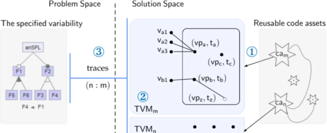
code assets of a given variability-rich system. It supports the following tasks, which are also depicted inFigure 5: 1. Capturing the imperfectly modular variability of code assets in terms of vp-s with variants, as abstract concepts. 2. Modeling this variability in terms of vp-s with variants while keeping the consistency with their implementation
in code assets.
3. Establishing the trace links between the specified and implemented variabilities.
The first two steps are mostly based on a conducted study of 21 variability implementation techniques regarding their 24 characteristic properties [87]. This study was briefly discussed inSection 2.2.3. We use this large set of summarized characteristic properties to understand what characterizes the variability in implementation and how it can be captured and modeled in terms of variation points with variants. Notably, we first analysed what characterizes only traditional techniques, being the focus of our study (cf.Section 2.2.3), which lead to the form of imperfect modularity of variability. Then, we noticed that 4 from the 21 characteristic properties are crucial for a variability management framework, namely for consistency checking, by which we would address𝐶ℎ𝑎𝑙𝑙𝑒𝑛𝑔𝑒2. Those four properties are the
Figure 5: A three step framework for variability management of code assets of a given variability-rich system. 𝖳𝖵𝖬𝑚
stands for technical variability model of the reusable code asset 𝖼𝖺𝗆, with vp-s {𝗏𝗉𝖺,𝗏𝗉𝖻, ...} and their respective variants
{𝗏𝖺𝟣,𝗏𝖺𝟤, ...} that are realized by different techniques {𝗍𝖺,𝗍𝖻, ...}. Whereas, {𝖿𝟣,𝖿𝟤, ...} are features in theFM.
logical relationbetween variants of a vp, their binding time, evolution, and granularity. On the other hand, the third step regarding the trace of variabilities is based on some other existing frameworks on variability traceability [4,5].
The second or third step begins only after the completion of its preceding step. In the following, we give a detailed and formal representation of each of these three steps, which are illustrated by examples.
4.1. Capturing the variability of code assets
As previously discussed, a variable part in code assets that has a form of imperfect modularity usually consists of a common part with its variants (cf.Figure 2b). It may happen that a whole code asset, such as a source file, a package, or a class, is a common part or varies (i.e., is a variant). In effect, the variable part consists of an implementation technique that denotes a mechanism for factorizing the commonality among related variants, for creating the variants, a way for resolving the variants, and the variants themselves. Toward addressing the first step of the framework, we naturally abstract them by using the concepts of variation points (vp-s) with variants. In general, it is expected that some targeted code assets of a system can have several vp-s and their variants, which can have dependencies with the vp-s and variants in the same or in other assets. Therefore,
Definition 2. Capturing the variability of code assets means to abstract the places where the variability happens,
namely the common code assets, or their common elements, with their varying code assets or their varying elements, and to represent them by variation points (vp-s) with variants concepts, respectively.
Capturing a vp with its variants is specific to the used technique to implement variability. Therefore, we propose the following formalization. Let 𝗏𝗉𝗑 be a specific variation point and 𝗏𝗑𝗒one of its variants, where 𝗑, 𝗒 ∈ ℕ. We
assume that the 𝗏𝗉𝗑is implemented by a single traditional technique𝗍𝗑. The setTof possible techniques for 𝗏𝗉𝗑with
its variants is then made explicit in our framework:
T = {𝗂𝗇𝗁𝖾𝗋𝗂𝗍𝖺𝗇𝖼𝖾, 𝗀𝖾𝗇𝖾𝗋𝗂𝖼 𝗍𝗒𝗉𝖾, 𝗈𝗏𝖾𝗋𝗋𝗂𝖽𝗂𝗇𝗀, 𝗈𝗏𝖾𝗋𝗅𝗈𝖺𝖽𝗂𝗇𝗀, 𝗌𝗍𝗋𝖺𝗍𝖾𝗀𝗒 𝗉𝖺𝗍𝗍𝖾𝗋𝗇, 𝗍𝖾𝗆𝗉𝗅𝖺𝗍𝖾 𝗉𝖺𝗍𝗍𝖾𝗋𝗇, ...}
It includes any traditional technique that promotes a form of reusability for code assets in a given variability-rich system2.
A vp with variants is not a by-product of such a traditional technique [20,81]. Therefore, to capture them properly, we need also to tag them in code assets in some way. In this context,
Definition 3. Tagging a variation point or variant means to map the variation point or variant concept to its concrete
asset, or asset element, in code assets.
2Although this set includes any of such techniques from object-oriented, functional programming, or design patterns, we exemplify and validate
the framework with a limited set of them. In total, we use up to ten techniques, which are common and are used in our considered variability-rich systems (given inSection 6).
This mapping is needed to keep the association between the captured vp or variant concept and its respective code asset.
For examplea, fromListing 1, the superclass AbstractLine2D is a vp and we abstract/capture it as vp_AbsLine2D. Whereas, tagging has in purpose to ensure their association, namely (AbstractLine2D, vp_AbsLine2D). Similarly, its subclasses StraightLine2D, LineSegment2D, and Ray2D are the vp’s variants, which we abstract as v_Line2D, v_Segment2D, and v_Ray2D, respectively. Their respective associations are: (StraightLine2D, v_Line2D), (LineSegment2D, v_Segment2D), and (Ray2D, v_Ray2D).
aIn the following, all illustrative examples will be given into similar blue boxes.
4.1.1. Tagging properties
We provide the following nomenclature for describing the tagging properties of vp-s with variants. Let the set𝖵𝖯of variation points in code assets of a targeted system be:
𝖵𝖯= {𝗏𝗉𝖺,𝗏𝗉𝖻,𝗏𝗉𝖼, ...,𝗏𝗉𝗇},where 𝖺, 𝖻, 𝖼, 𝗇 ∈ℕ (1) The set𝖵of all realized variants for the𝗏𝗉𝗑∈ 𝖵𝖯is then:
𝖵= {𝗏𝗑𝟣,𝗏𝗑𝟤,𝗏𝗑𝟥, ...,𝗏𝗑𝗇},where 𝗑, 𝗇 ∈ℕ (2)
The set𝖢𝖠of all code assets of the system, with variability or being variable themselves, which have an association to some vp-s or their variants, is:
𝖢𝖠= {𝖼𝖺𝗆,𝖼𝖺𝗇,𝖼𝖺𝗈, ...,𝖼𝖺𝗓},where 𝗆, 𝗇, 𝗈, 𝗓 ∈ℕ. (3) The set of elements in a code asset, for example, for𝖼𝖺𝗑 ∈ 𝖢𝖠, which have an association to some vp-s or their variants, is:
𝖼𝖺𝗑 = {𝖾𝖺𝗑𝟣,𝖾𝖺𝗑𝟤,𝖾𝖺𝗑𝟥, ...,𝖾𝖺𝗑𝗇},where 𝗑, 𝗇 ∈ℕ. (4)
According toDefinition 3, the abstractions of each vp and variant from sets (1) and (2) are associated with their concrete implementation in code assets, for example, with a varying file, class, or method, which we named as in sets (3) and (4). Analysing some of the traditional variability implementation techniques, we discerned five possible associations for vp-s and five for variants. They also represent all possible associations between a vp or a variant and their respective code assets. All these associations are described in the following and can be grouped into three kinds, named as single location, implicit, or spread.
Single location.
This kind of association represents the case when a vp or variant is tagged to a single location in code assets. The four possible cases are:• (𝗏𝗉𝗑,𝖼𝖺𝗑)or (𝗏𝗉𝗑,𝖾𝖺𝗑𝗇), when the code asset 𝖼𝖺𝗑or the 𝑛 element of it is a common part of some variants. This is
the case when 𝗏𝗉𝗑is associated with only one code asset or with only one element of a code asset, respectively.
For instance, the association (vp_AbsLine2D, AbstractLine2D ) is between the vp and the class, as a code asset or an element of a file, that implements it.
• (𝗏𝗑𝗒,𝖼𝖺𝗑)or (𝗏𝗑𝗒,𝖾𝖺𝗑𝗇), where 𝗒 in𝗏𝗑𝗒represents a specific variant of 𝖵 in (2) and 𝗇 represents a specific varying
code asset of 𝖢𝖠 in (3) or a varying element of 𝖼𝖺𝗑in (4). This is the case when the variant is associated with
only one varying asset or one varying element of it.
(v_Line2D, StraightLine2D ), (v_Segment2D, LineSegment2D ), or (v_Ray2D, Ray2D ), where each of these variants is implemented by a single class in code assets.
Implicit.
This kind of association represents the case when a vp or variant is implicit and cannot easily be tagged in code assets. Therefore,• (𝗏𝗉𝗑,∅)or (𝗏𝗑𝗒,∅), when the 𝗏𝗉𝗑or 𝗏𝗑𝗒is implicit, that is, hard to be tagged.
For example, this is the case when an if-else statement is used [84].
We do not include in the framework two cases: (i) the case when a vp is introduced but has no variants [84], as we consider that it is part of the core assets [91], and (ii) the case when a variant is unimplemented, because, for example, an abstract class may have infinite subclasses as variants and abstracting them would be impossible.
Spread.
This kind of association represents the case when the same vp or variant is tagged to several locations in code assets. Therefore,• (𝗏𝗉𝗑,{𝖼𝖺𝗆,𝖼𝖺𝗇, ...,𝖼𝖺𝗓})or (𝗏𝗉𝗑,{𝖾𝖺𝗑𝟣,𝖾𝖺𝗑𝟤, ...,𝖾𝖺𝗑𝗇}), when the 𝗏𝗉𝗑 is found in more than one place in code
assets. The 𝗏𝗉𝗑 can be associated also with any code asset from the set 𝖢𝖠 in (3) and/or with any of their
elements from the set 𝖼𝖺𝗑in (4).
• (𝗏𝗑𝗒,{𝖼𝖺𝗆,𝖼𝖺𝗇, ...,𝖼𝖺𝗓})or (𝗏𝗑𝗒,{𝖾𝖺𝗑𝟣,𝖾𝖺𝗑𝟤, ...,𝖾𝖺𝗑𝗇}), when the variant is found in more than one place in code
assets. The 𝗏𝗑𝗒can be associated also with any code asset from the set 𝖢𝖠 in (3) and/or with any of their elements
from the set 𝖼𝖺𝗑in (4).
This is the case when a vp or variant is implemented by more than one core asset or their elements. For ex-ample, the (vp_distance, {distance(p), distance(x, y) }) is a vp that encircle both overriden methods, therefore it needs to be tagged to both of them.
Moreover, these spread cases have a slightly different meaning from the crosscutting case of features, for example, when preprocessor directives are used. Commonly, preprocessors are used to annotate the lines of code that implement the functionality of a domain feature, which may crosscut the current design of code. Whereas, we consider that vp-s and variants align with the design of code.
In some existing approaches vp-s or variants are labeled depending on their resolution nature (e.g., choice, sub-stitution [40]), or depending on their location in assets (e.g., kernel-param-vp, kernel-abstract-vp [37]). For now, we keep a more inclusive label, simply as a vp and variant concept, which can reflect in the future their resolution nature, location, or evolution.
4.1.2. Capturing characteristic properties
In addition to the tagging properties, depending on the used variability implementation technique, the nature of a code asset element that represents a vp or one of its variants varies. Their variety is presented by the characteristic properties of vp-s with variants [87]. Therefore, as part of our framework, we introduce here a formal definition of four properties that need to be captured, given that they are essential for variability management, such as for checking, resolving, and evolving the variability. They are the logical relations between variants in a vp, or between vp-s, their binding time, evolution, and granularity.
Logical relation.
The logical relations between variants in a 𝗏𝗉𝗑variation point that are commonly faced in practice are similar to the relations between features in anFM(cf. Section 2.1). In addition, vp-s with variants can have dependencies [21], which are also similar to the dependencies between features in anFM, such as mutual exclusion, and requires. All these possible relations are shown inTable 1.A single technique, 𝗍𝗑 ∈T, can offer at least one of these logical relations between variants. For example,
inheri-tance can be used for implementing the alternative variants, overriding for implementing the or variants, or aggregation for implementing the optional variant(s) of a vp.
Concretely, after the three variants v_Line2D, v_Segment2D, and v_Ray2D inListing 1are tagged, we capture their alternativelogical relation, which is realized by inheritance.
Table 1
Logical relations of variation points and of variants in a variation point. Logical Relation Description
Mandatory The variation point or variant is part of each software product
Optional The variation point or variant can be part of the software product or not
Multi Coexisting (Or) One or more than one of the variants in a variation point can be part of the software product Alternative (Xor) Only one of the alternative variants in a variation point can be part of the software product Mutual exclusion When, during configuration, the selection of variation point or variant requires the exclusion
of another variation point or variant, and vice versa
Requires When the selection of a variation point or variant requires the selection of another variation points or variant
Table 2
Binding times of variation points with variants. Source: Adapted from [19,22].
Binding time Values Description
Static binding (S) (S) compilation / link (S) build / assembly (S) programming time (S/D) configuration (S/D) deploy and redeploy
The variability is resolved early during the development cycle, that is, the decision for a variant in a variation point is made early/statically.
Dynamic binding (D) (D) runtime (start-up) (D) pure runtime (operational mode)
The variability is resolved later during the development cycle, that is, the decision for a variant in a variation point is made as late as possible/dynamically.
Therefore, we define the set of possible logical relations (LG) of vp-s and of variants in a vp as: LG = {𝗆𝖺𝗇𝖽𝖺𝗍𝗈𝗋𝗒, 𝗈𝗉𝗍𝗂𝗈𝗇𝖺𝗅, 𝖺𝗅𝗍𝖾𝗋𝗇𝖺𝗍𝗂𝗏𝖾, 𝗈𝗋, 𝗆𝗎𝗍𝗎𝖺𝗅 𝖾𝗑𝖼𝗅𝗎𝗌𝗂𝗈𝗇, 𝗋𝖾𝗊𝗎𝗂𝗋𝖾𝗌}
Binding time.
Within the code assets of a system, each vp is associated with a binding time, which is the time when the variability is decided or the vp is resolved with its variants during a product derivation. Then, different vp-s may require being resolved at different development phases. Generally, depending from the chosen variability implementation technique, a vp can be resolved early during the development cycle (e.g., statically, when the decision for a variant is made at compile time), or later during the development cycle (e.g., dynamically, at runtime) [18,3,41]. In some domains, a vp may require more than one binding time (i.e., multiple binding times), for example when a feature requires a static and/or a dynamic binding [77]. In this case, it represents a real challenge for existing techniques, as they offer only a single binding time. To accomplish a flexible binding time, different techniques are usually required to be combined. However, these cases seem to be very specific and rare. On the other hand, there are distinguished binding units, which are important for identifying which vp-s should be bound together. Specifically, when several vp-s participate in implementing some major functionality in a system then they may require to be resolved together as a unit [22, Ch. 4],[56,55]. Therefore in this work, we consider that a vp with its variants is realized by a single variability implementation technique that offers a single binding time and is bound independently.The binding time here is the time when the variability should be resolved and should not be confused with the time when it will be introduced, which is differentiated by Svahnberg et al. [84]. As for the common kinds of binding times, a taxonomy is available [22,19]. While some approaches have a broader view on binding times, for instance, advocating for different binding times at runtime [19,41], we use the seven most common static and dynamic binding times in our model, as shown inTable 2.
Thus, the set of possible static and dynamic binding times (BT) of a 𝗏𝗉𝗑is:
Table 3
Granularity of variation points and of their variants.
Granularity Values Description
Coarse-grained Component, framework with plug-ins as vari-ants, file, package, class, interface, etc.
The specified variability has an effect on the coarsest grained elements of the implementation structure. Medium-grained Method, field inside a class, etc. The specified variability has an effect on the medium
grained elements of the implementation structure. Fine-grained Expression, statement, block of code within
a method, generic type, argument, etc.
The specified variability has an effect on the finest grained elements of the implementation structure.
For example, inListing 1we capture that the vp_AbsLine2D is bound during the runtime to one of its three alternative variants, for instance, to v_Segment2D.
Evolution.
Depending on whether the specified variability in theFMis meant to be evolved with new features, new vp-s may emerge or a specific vp may evolve with new variants in the future. Thus, depending on the used technique, the new or existing vp-s can be open or closed to evolution.Therefore, the evolution set (EV) is:
EV = {𝗈𝗉𝖾𝗇, 𝖼𝗅𝗈𝗌𝖾𝖽}
For example, we capture a vp as closed when it is implemented as an enum type in Java, and open when it is implemented simply as an abstract class.
In the JavaGeom system, the abstract class vp_AbstractLine2D inListing 1is a vp that we capture as an open vp_AbsLine2D, meaning that its variants can evolve in the future.
Granularity.
A vp or variant in code assets can have a specific granularity depending on the size of variability and the used technique [6, p.59][50]. Specifically, a vp or variant, as abstractions of variability, may represent (i) a coarse-grained element that is going to vary, such as a file, a package, a class, or an interface, (ii) a medium-grained element, such as a method, or a field inside a class, or (iii) a fine-grained element, such as an expression, a statement, or a block of code. A summary of them is provided inTable 33. Thus, when traditional techniques are used, thefollowing granularity set (GR) contains the elements that actually show the granularity levels at which a variability implementation technique may be used to implement a vp or variant.
GR = {𝖿𝗂𝗅𝖾, 𝗉𝖺𝖼𝗄𝖺𝗀𝖾, 𝗂𝗇𝗍𝖾𝗋𝖿𝖺𝖼𝖾, 𝖼𝗅𝖺𝗌𝗌, 𝗆𝖾𝗍𝗁𝗈𝖽, 𝖿𝗂𝖾𝗅𝖽, 𝗌𝗍𝖺𝗍𝖾𝗆𝖾𝗇𝗍, 𝗀𝖾𝗇𝖾𝗋𝗂𝖼 𝗍𝗒𝗉𝖾, 𝖺𝗋𝗀𝗎𝗆𝖾𝗇𝗍, ...}
For example, inListing 1we should be able to capture the variant v_Line2D in class level, which is realized by the class StraightLine2D in lines 21-24; or, the variant v_distance in method level, which is realized by distance(...) method in lines 6-9 or 11-18.
4.2. Modeling the variability of code assets
Given that each captured vp with its variants is realized by a single technique, they are then somehow related. For example, inListing 1the three variants, 𝗏_𝖫𝗂𝗇𝖾𝟤𝖣, 𝗏_𝖲𝖾𝗀𝗆𝖾𝗇𝗍𝟤𝖣, and 𝗏_𝖱𝖺𝗒𝟤𝖣, are related by inheritance with the 𝗏𝗉_𝖠𝖻𝗌𝖫𝗂𝗇𝖾𝟤𝖣, which technique offers an alternative relationship between variants, a runtime binding of variants, and an open evolution of the vp itself.
3A similar table, which also includes the granularity of language constructs coming from the emerging techniques, such as feature modules as
Therefore, we model their relation by associating each vp with its realized variants and the used implementation technique. The associated technique 𝗍𝗑∈T of the 𝗏𝗉𝗑∈𝖵𝖯, which relation we write as (𝗏𝗉𝗑,𝗍𝗑), describes three main
properties of the 𝗏𝗉𝗑: the logical relation for its variants (𝗅𝗀𝗑), the binding time (𝖻𝗍𝗑), and the evolution (𝖾𝗏𝗑):
𝗍𝗑= {𝗅𝗀𝗑,𝖻𝗍𝗑,𝖾𝗏𝗑, ...}, where 𝗅𝗀𝗑∈LG, 𝖻𝗍𝗑∈BT, and 𝖾𝗏𝗑∈EV
The three dots in 𝗍𝗑indicate that the other properties can be added, such as the granularity level. Based on the above
example, we can establish
𝗂𝗇𝗁𝖾𝗋𝗂𝗍𝖺𝗇𝖼𝖾= {𝖺𝗅𝗍𝖾𝗋𝗇𝖺𝗍𝗂𝗏𝖾, 𝗋𝗎𝗇𝗍𝗂𝗆𝖾, 𝗈𝗉𝖾𝗇, ...}
In this way, we aim to address the second step of our framework (cf.Figure 5) for modeling the implemented vari-ability while keeping the association among the vp-s with variants, their implementation techniques, and the elements of code asset that they abstract.
4.2.1. Types of variation points
For modeling the implemented variability, we observed that the following five types of vp-s can be distinguished. They are given in the setXbelow.
X = {𝗏𝗉, 𝗏𝗉_𝗎𝗇𝗂𝗆𝗉𝗅𝖾𝗆𝖾𝗇𝗍𝖾𝖽, 𝗏𝗉_𝗍𝖾𝖼𝗁𝗇𝗂𝖼𝖺𝗅, 𝗏𝗉_𝗇𝖾𝗌𝗍𝖾𝖽, 𝗏𝗉_𝗈𝗉𝗍𝗂𝗈𝗇𝖺𝗅}
This is not an exhaustive list of them, other types of vp-s may also be possible, but this set was proved to be sufficient during the framework application (cf.Section 6). A formalization for each of them is given in the following.
Ordinary.
An ordinary variation point (vp) is an introduced and implemented vp by a specific technique, including all its variants, which are also implemented. Therefore, when the 𝗏𝗉𝗑 is an ordinary vp we model this variability incode assets as a set of its variants and the characteristic properties derived from the 𝗏𝗉𝗑’s implementation technique,
𝗍𝗑. This leads to the following definition (cf.Equations (1)and(2)):
𝗏𝗉𝗑= {𝖵, 𝗍𝗑} = {{𝗏𝗑𝟣,𝗏𝗑𝟤,𝗏𝗑𝟥, ...,𝗏𝗑𝗇}, 𝗍𝗑},where 𝗇 ∈ℕ (5)
Based on this, we propose the following graphical representation of it4:
(𝗏𝗉𝗑,𝗍𝗑) 𝗏𝗑𝟣 𝗏𝗑𝟤 𝗏𝗑𝟥 ...
≡
(𝗏𝗉𝗑,{𝗅𝗀𝗑,𝖻𝗍𝗑,𝖾𝗏𝗑, ...}) 𝗏𝗑𝟣 𝗏𝗑𝟤 𝗏𝗑𝟥 ... Such ordinary vp with its variants, fromListing 1, is:
(𝗏𝗉_𝖠𝖻𝗌𝖫𝗂𝗇𝖾𝟤𝖣, {𝖺𝗅𝗍𝖾𝗋𝗇𝖺𝗍𝗂𝗏𝖾, 𝗋𝗎𝗇𝗍𝗂𝗆𝖾, 𝗈𝗉𝖾𝗇}) 𝗏_𝖫𝗂𝗇𝖾𝟤𝖣 𝗏_𝖲𝖾𝗀𝗆𝖾𝗇𝗍𝟤𝖣 𝗏_𝖱𝖺𝗒𝟤𝖣
Unimplemented.
An unimplemented variation point (vp) is an introduced vp but without predefined variants, mean-ing that its variants are unknown durmean-ing the domain engineermean-ing phase. When the 𝗏𝗉𝗑 is an unimplemented vp, wemodel it as:
𝗏𝗉𝗑= {{∅}, 𝗍𝗑} (6)
respectively,
(𝗏𝗉𝗑,𝗍𝗑)
4To easily show the main distinction between the five types of vp-s, we use this representation (for simplicity, mostly only its left side). Whereas,
It means that 𝗏𝗉𝗑is introduced by the technique 𝗍𝗑, whereas its variants will be implemented later.
Technical.
A technical variation point (vp) is introduced and implemented only for supporting internally the imple-mentation of another vp which has a direct mapping to a domain feature. The mere difference with the other vp-s is that it does not have a direct mapping to a domain feature, thus the name technical. Moreover, a technical vp is in principle an ordinary vp and needs to be modeled at the implementation level as it needs, for example, to be resolved during product derivation. For the sake of generalization, we consider that a technical vp can also be an unimplemented vp. When a technical variation point 𝗏𝗉𝗒is within a variant 𝗏𝗑𝟥of an ordinary 𝗏𝗉𝗑, it is modeled as below.𝗏𝗉𝗑= {{𝑣𝑥1, 𝑣𝑥2, 𝑣𝑥3, ..., 𝑣𝑥𝑛}, 𝑡𝑥} 𝗏𝗉𝗒= {{𝑣𝑦1, 𝑣𝑦2, 𝑣𝑦3, ..., 𝑣𝑦𝑛}, 𝑡𝑦} where 𝗇 ∈ℕ and 𝗏𝗉𝗒 ⊂ 𝑣𝑥3 (7) respectively, (𝗏𝗉𝗑,𝗍𝗑) 𝗏𝗑𝟣 𝗏𝗑𝟤 𝗏𝗑𝟥 (𝗏𝗉𝗒,𝗍𝗒) 𝗏𝗒𝟣 𝗏𝗒𝟤 𝗏𝗒𝟥 ... ...
For example, let us consider that vp_distance is the abstraction of the method level variability inListing 1. It can be considered as a technical vp of vp_AbsLine2D, within the variant v_Line2D, as it is not modeled in theFM. It has two alternative variants, v_distPoint2D (cf. lines 6-9) and v_distDouble (cf. lines 11-18), which are realized using the technique of overloading. This variability is then modeled as follows.
(𝗏𝗉_𝖠𝖻𝗌𝖫𝗂𝗇𝖾𝟤𝖣, {𝖺𝗅𝗍𝖾𝗋𝗇𝖺𝗍𝗂𝗏𝖾, 𝗋𝗎𝗇𝗍𝗂𝗆𝖾, 𝗈𝗉𝖾𝗇}) 𝗏_𝖫𝗂𝗇𝖾𝟤𝖣
(𝗏𝗉_𝖽𝗂𝗌𝗍𝖺𝗇𝖼𝖾, {𝖺𝗅𝗍𝖾𝗋𝗇𝖺𝗍𝗂𝗏𝖾, 𝖼𝗈𝗆𝗉𝗂𝗅𝖾, 𝗈𝗉𝖾𝗇}) 𝗏_𝖽𝗂𝗌𝗍𝖯𝗈𝗂𝗇𝗍𝟤𝖣 𝗏_𝖽𝗂𝗌𝗍𝖣𝗈𝗎𝖻𝗅𝖾
𝗏_𝖲𝖾𝗀𝗆𝖾𝗇𝗍𝟤𝖣 𝗏_𝖱𝖺𝗒𝟤𝖣
Nested.
A nested variation point (vp) represents a variable part in a code asset which becomes the common part for some other variants. On the contrary to a technical vp, when the 𝗏𝗉𝗒is a nested variation point of 𝗏𝗉𝗑then a variablepart (e.g., the variant 𝗏𝗑𝟥) becomes the common part for the variability of 𝗏𝗉𝗒 (e.g., for 𝗏𝗒𝟣, 𝗏𝗒𝟤, and 𝗏𝗒𝟥). This is
modeled as follows.
𝗏𝗉𝗑 = {{𝑣𝑥1, 𝑣𝑥2, 𝑣𝑥3, ..., 𝑣𝑥𝑛}, 𝑡𝑥} = {{𝑣𝑥1, 𝑣𝑥2,𝗏𝗉𝗒, ..., 𝑣𝑥𝑛}, 𝑡𝑥} = = {{𝑣𝑥1, 𝑣𝑥2,{{𝑣𝑦1, 𝑣𝑦2, 𝑣𝑦3, ..., 𝑣𝑦𝑛}, 𝑡𝑦}, ..., 𝑣𝑥𝑛}, 𝑡𝑥} where 𝗇 ∈ℕ and 𝑣𝑥3≡ 𝗏𝗉𝗒
respectively,
(𝗏𝗉𝗑,𝗍𝗑) 𝗏𝗑𝟣 𝗏𝗑𝟤 𝗏𝗑𝟥≡ (𝗏𝗉𝗒,𝗍𝗒)
𝗏𝗒𝟣 𝗏𝗒𝟤 𝗏𝗒𝟥 ... ...
For example, v_Line2D can be a vp for its (un)implemented variants. (𝗏𝗉_𝖠𝖻𝗌𝖫𝗂𝗇𝖾𝟤𝖣, {𝖺𝗅𝗍𝖾𝗋𝗇𝖺𝗍𝗂𝗏𝖾, 𝗋𝗎𝗇𝗍𝗂𝗆𝖾, 𝗈𝗉𝖾𝗇}) 𝗏_𝖫𝗂𝗇𝖾𝟤𝖣 ≡ (𝗏𝗉𝗒,𝗍𝗒) 𝗏_𝖲𝖾𝗀𝗆𝖾𝗇𝗍𝟤𝖣 𝗏_𝖱𝖺𝗒𝟤𝖣
Optional.
An optional variation point (vp) represents a vp in code assets that together with its all variants is optional. This means that, whenever an optional vp is included or excluded in a software product, so are its variants. Moreover, variants may have any of the logical relations among themselves.In our framework, when 𝗏𝗉𝗑is optional then we represent the (𝗏𝗉𝗑, 𝗍𝗑) tuple as a triple, that is, (𝗏𝗉𝗑, 𝗍𝗑, 𝗈𝗉𝗍). We
use the acronym 𝗈𝗉𝗍 here in order to distinguish the optionality of the vp itself, which is different from the optional logical relation among variants in a vp. An optional vp can be ordinary, unimplemented, and can have other nested or technical vp-s. This is modeled as:
(𝗏𝗉𝗑,𝗈𝗉𝗍) = {{𝑣𝑥1, 𝑣𝑥2, 𝑣𝑥3, ..., 𝑣𝑥𝑛}, 𝑡𝑥},where 𝗇 ∈ℕ (9) respectively,
(𝗏𝗉𝗑,𝗍𝗑,𝗈𝗉𝗍)
𝗏𝗑𝟣 𝗏𝗑𝟤 𝗏𝗑𝟥 ...
To make a vp as optional it may not require a technique, that is, simply the vp with its variants is not included in the final software product. Therefore, we should document/model it.
4.2.2. Fragmented variability modeling
In addition to the logical relation among variants in a vp, different vp-s and their variants may also be related, for instance, the nested, technical, and/or ordinary vp-s with their variants. This implies that the whole modeled variability at the implementation level will have a forest-like structure, where the vp-s and their variants that are related will belong to the same tree, whereas those that are not related will belong to different trees.
In our framework, instead of modeling the whole implemented variability at once and in one place, we propose to model it in a fragmented way. That is, each fragment may include at least one tree with a vp and its variants. While there is a problem of reconciliation between evolving code and variabilities with separate models, we choose this solution for three reasons: (i) to follow the expected forest-like structure of variability in code assets, (ii) to take into account the large amount of implemented variability in real systems, which can be even larger than the domain variability (capturing it in a single model may hamper scalability), and (iii) to be able to reason locally over a fragment, for example, to check its consistency. Moreover, instead of a traditional global variability model for a variability-rich system, a modular variability model opens the path toward the development of software ecosystems and product lines of product lines [52]. What we consider as a fragment aims at being flexible. Specifically, it is a code asset with variability, which can be a package, a file, or a class. In other words, a fragment can be any unit that has its inner variability and it is worth being modeled locally or separately.
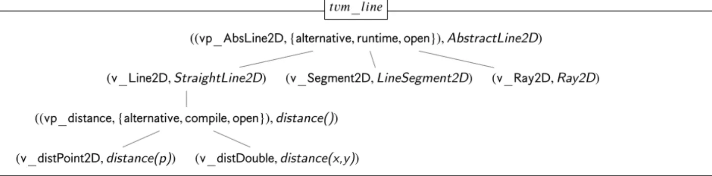
((𝗏𝗉_𝖠𝖻𝗌𝖫𝗂𝗇𝖾𝟤𝖣, {𝖺𝗅𝗍𝖾𝗋𝗇𝖺𝗍𝗂𝗏𝖾, 𝗋𝗎𝗇𝗍𝗂𝗆𝖾, 𝗈𝗉𝖾𝗇}), AbstractLine2D) (𝗏_𝖫𝗂𝗇𝖾𝟤𝖣, StraightLine2D) ((𝗏𝗉_𝖽𝗂𝗌𝗍𝖺𝗇𝖼𝖾, {𝖺𝗅𝗍𝖾𝗋𝗇𝖺𝗍𝗂𝗏𝖾, 𝖼𝗈𝗆𝗉𝗂𝗅𝖾, 𝗈𝗉𝖾𝗇}), distance()) (𝗏_𝖽𝗂𝗌𝗍𝖯𝗈𝗂𝗇𝗍𝟤𝖣, distance(p)) (𝗏_𝖽𝗂𝗌𝗍𝖣𝗈𝗎𝖻𝗅𝖾, distance(x,y)) (𝗏_𝖲𝖾𝗀𝗆𝖾𝗇𝗍𝟤𝖣, LineSegment2D) (𝗏_𝖱𝖺𝗒𝟤𝖣, Ray2D) 𝑡𝑣𝑚_𝑙𝑖𝑛𝑒
Figure 6: Documentation of the implemented variability in a𝖳𝖵𝖬for the JavaGeom PL (cf.Listing 1). The italic names stand for tags of vp-s and variants to the variable asset elements.
For this reason, we propose to model the variability of each fragment in a separate model, named as technical variability models(𝖳𝖵𝖬). It will contain the abstractions of vp-s with variants, tags to their respective code asset elements, and their characteristic properties within some given code assets. Then, a𝖳𝖵𝖬is the power set of all vp-s in some given code assets. For example, let us suppose that the vp-s in (1) capture the variability of the code asset 𝖼𝖺𝗑
in (3) and (4), then the𝖳𝖵𝖬𝗑is:
𝖳𝖵𝖬𝗑 = 𝖯𝗈𝗐(𝖵𝖯𝗑) ={{{𝗏𝖺𝟣,𝗏𝖺𝟤, ...,𝗏𝖺𝗇}, 𝗍𝖺}, {{𝗏𝖻𝟣,𝗏𝖻𝟤, ...,𝗏𝖻𝗇}, 𝗍𝖻}, ...,{{𝗏𝗓𝟣,𝗏𝗓𝟤, ...,𝗏𝗓𝗇}, 𝗍𝗓}} (10) where 𝖺, 𝖻, 𝗇, 𝗑, 𝗓 ∈ℕ.
As a result, the whole existing variability of code assets of a system, that is, of 𝖢𝖠 inEquation (3), is modeled in technical variability models (𝖳𝖵𝖬s). It is important to note that, for simplicity, the tags of variants to the variable asset elements in the 𝖳𝖵𝖬𝗑inEquation (10)are not shown, while they are illustrated inFigure 6. This is because, as specified
inSection 4.1.1, any of the variants in 𝖳𝖵𝖬𝗑can have one or more tags to the reusable code assets inEquation (3)
and/orEquation (4).
In a more illustrative way, inFigure 6 is shown the 𝗍𝗏𝗆_𝗅𝗂𝗇𝖾 that model the implemented variability inListing 1. Specifically, it shows the two vp-s, the ordinary vp_AbsLine2D and the technical vp_distance, with their variants and tags to the variable asset elements for the excerpt of JavaGeom system. Similarly, the remained variability in JavaGeom can be modeled within the same or in other𝖳𝖵𝖬s.
A different number of𝖳𝖵𝖬s can be used in a given system, while all of them together model the variability of its all code assets. Conceptually, all𝖳𝖵𝖬s constitute the main technical variability model (𝖬𝖳𝖵𝖬), which is specific to the given system. As part of our framework, the𝖬𝖳𝖵𝖬can be defined as the set of all𝖳𝖵𝖬s, given in the following.
𝖬𝖳𝖵𝖬= {𝖳𝖵𝖬𝗆,𝖳𝖵𝖬𝗇,𝖳𝖵𝖬𝗈, ...,𝖳𝖵𝖬𝗓} (11) Thus, the𝖬𝖳𝖵𝖬contains the modeled variability of all code assets of a given system. Moreover, unlike the organi-zation of features in an 𝖥𝖬 as a tree structure, vp-s with variants in the𝖬𝖳𝖵𝖬reside in a forest-like structure.
Based on these two steps of the framework, we noticed that the original meaning of a vp given inSection 2.2.2 can be further refined:
Definition 4. A variation point is a location in code assets of a system that represents a node for collecting, attaching
to the core implementation, and configuring a set of variable units (variable elements of code assets) that are related in functionality. In particular, it is the place at which the variation occurs [45] and represents the used technique to realize the variability.
4.3. Tracing the variability of reusable code assets
Variability traceability is usually organized around two types of trace links: realization and use [5,75]. The first type of links is used in domain engineering for relating the specified variability at the domain level with the artifacts
Figure 7: 1-to-1 mapping: ideal mapping. Figure 8: 1-to-1 mapping: a special case of this mapping.
that realize it, such as in code level. Similar usage of this type of link can be found for example between application and platform features [58]. The use type of links relates an artifact during the application engineering process to its respective core assets that are developed during the domain engineering process [75]. It is used to show from which core assets an artifact is elicited during product derivation. Usually, the realization trace link is implied by "variability traceability" and in the same meaning we use it also here, for the third step of our framework.
4.3.1. Realization trace links
Let us suppose that𝖿𝗑∈𝖥𝖬is a domain feature of a given system, then
𝖥𝖬= {𝖿𝟣,𝖿𝟤,𝖿𝟥, ...,𝖿𝗇}, where 𝗇 ∈ ℕ (12) is the set of features in its feature model (𝖥𝖬). In a similar way with the illustration of a vp with variants during the framework’s first two steps, a compound feature 𝖿𝗑with its varying features and their logical relation (i.e., logic) can
be given in an illustrative way as follows. The logic can have any of the values fromTable 1inSection 4.1.2. (𝖿𝗑,𝗅𝗈𝗀𝗂𝖼)
𝖿𝗑𝟣 𝖿𝗑𝟤 𝖿𝗑𝟥 ...
For mapping features of an 𝖥𝖬 to vp-s and variants of𝖳𝖵𝖬s we use a single bidirectional type of trace links implementedBy(⟼) or implements (⟵∣), which presents the variability realization trace link at the implemen-tation level. Although the nature of trace links is bidirectional, a single bidirectional type is needed to distinguish which is the source artifact and which is the target artifact of the trace link (according to the trace link definition given inSection 2.3). Namely, implementedBy and implements make possible this differentiation. Otherwise, a link such as 𝖿𝗑 ↔ 𝗏𝗉𝗑would become hard to read as the source and target artifacts are not distinguished.
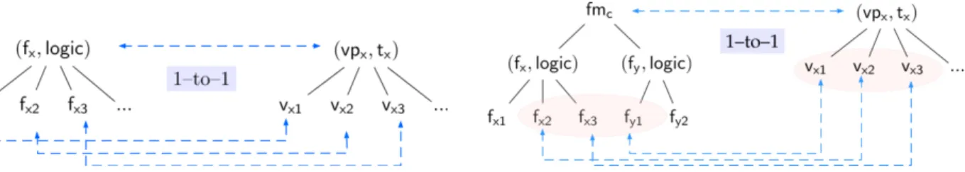
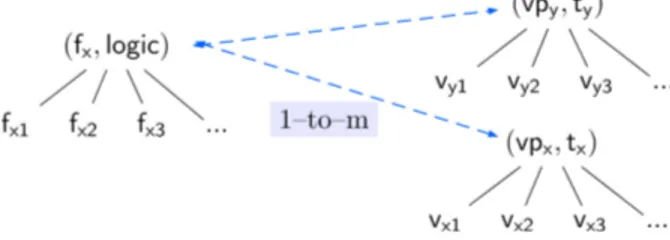
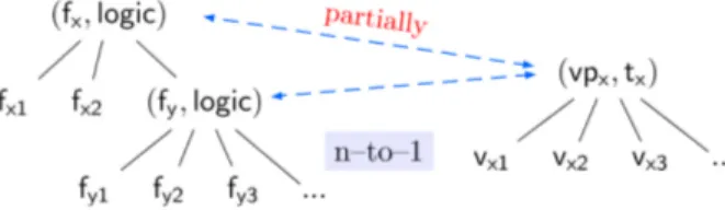
In general, this mapping of variability from the domain level to the implementation level is expected to be n-to-m (cf. step ® inFigure 5). For example, if a domain feature is implemented by three vp-s , then three trace links are needed to describe this mapping. Specifically, from the analysed diversity of vp-s with variants [87], traces of variability may consist of (1) 1-to-1 mapping, (2) 1-to-m mapping, and/or (3) n-to-1 mapping.
1-to-1 mapping.
This is the ideal mapping where each specified feature is realized by a single code asset (element), which is represented by a vp or variant concept. Such mapping looks as inFigure 7.In this case, we say that a compound feature 𝖿𝗑and its varying features 𝖿𝗑𝟣,𝖿𝗑𝟤, and 𝖿𝗑𝟥are implemented ideally by
a single variation point 𝗏𝗉𝗑 with its variants 𝗏𝗑𝟣,𝗏𝗑𝟤, and 𝗏𝗑𝟥, or conversely. Thus, their mapping is ideal or 1-to-1.
Therefore, for feature 𝖿𝗑we write:
(𝖿𝗑 ⟼ 𝗏𝗉𝗑)
implementedBy (𝖿𝗑,𝗏𝗉𝗑) implements (𝗏𝗉𝗑,𝖿𝗑)
(13)
For example, from Figures 1and3in JavaGeom, (StraightCurve2D ⟼ vp_AbsLine2D). That is, the feature StraightCurve2Dis implemented by the single variation point vp_AbsLine2D, thus mapped to it.
![Figure 1: An excerpt of the feature model (FM) of JavaGeom variability-rich system (The FM is created using the FeatureIDE tool [62]).](https://thumb-eu.123doks.com/thumbv2/123doknet/13565867.420640/3.816.255.562.86.203/figure-excerpt-feature-model-javageom-variability-created-featureide.webp)