HAL Id: hal-01136865
https://hal.archives-ouvertes.fr/hal-01136865
Submitted on 30 Mar 2015
HAL is a multi-disciplinary open access
archive for the deposit and dissemination of
sci-entific research documents, whether they are
pub-lished or not. The documents may come from
teaching and research institutions in France or
abroad, or from public or private research centers.
L’archive ouverte pluridisciplinaire HAL, est
destinée au dépôt et à la diffusion de documents
scientifiques de niveau recherche, publiés ou non,
émanant des établissements d’enseignement et de
recherche français ou étrangers, des laboratoires
publics ou privés.
estimation; its concepts and implementation for the
AMMA experiment
Jean-Claude Bergès, I. Jobard, F. Chopin, R. Roca
To cite this version:
Jean-Claude Bergès, I. Jobard, F. Chopin, R. Roca. EPSAT-SG: a satellite method for
precipita-tion estimaprecipita-tion; its concepts and implementaprecipita-tion for the AMMA experiment. Annales Geophysicae,
European Geosciences Union, 2010, 28 (1), pp.289-308. �10.5194/angeo-28-289-2010�. �hal-01136865�
www.ann-geophys.net/28/289/2010/
© Author(s) 2010. This work is distributed under the Creative Commons Attribution 3.0 License.
Annales
Geophysicae
EPSAT-SG: a satellite method for precipitation estimation; its
concepts and implementation for the AMMA experiment
J. C. Berg`es1, I. Jobard2,3, F. Chopin2, and R. Roca2
1PRODIG, Universit´e Paris 1, 75005 Paris, France
2LMD, IPSL/CNRS, Ecole Polytechnique, 91128 Palaiseau, France 3Univ. Paris-Sud, 92296 Chatenay, France
Received: 23 June 2009 – Revised: 7 October 2009 – Accepted: 31 October 2009 – Published: 27 January 2010
Abstract. This paper presents a new rainfall estimation
method, EPSAT-SG which is a frame for method design. The first implementation has been carried out to meet the require-ment of the AMMA database on a West African domain. The rainfall estimation relies on two intermediate products: a rainfall probability and a rainfall potential intensity. The first one is computed from MSG/SEVIRI by a feed forward neural network. First evaluation results show better proper-ties than direct precipitation intensity assessment by geosta-tionary satellite infra-red sensors. The second product can be interpreted as a conditional rainfall intensity and, in the described implementation, it is extracted from GPCP-1dd. Various implementation options are discussed and compari-son of this embedded product with 3B42 estimates demon-strates the importance of properly managing the temporal discontinuity. The resulting accumulated rainfall field can be presented as a GPCP downscaling. A validation based on ground data supplied by AGRHYMET (Niamey) indicates that the estimation error has been reduced in this process. The described method could be easily adapted to other geo-graphical area and operational environment.
Keywords. Meteorology and atmospheric dynamics
(Pre-cipitation; Tropical meteorology; Instruments and tech-niques)
1 Introduction
Rainfall is a key parameter both for energy cycle studies and environment monitoring. For example, early warning sys-tems in agronomy and epidemiology rely mainly on precipi-tation mapping and, despite a deep international commitment in this domain, getting this information timely and accurately
Correspondence to: J. C. Berg`es ([email protected])
is still a sensitive issue (Tefft et al., 2006). The global ground observation network is by no mean sufficient as it lacks the adequate density and data quality. Moreover such a network is costly to operate and only few land area, mostly concen-trated in mid-latitude, are properly covered. This issue is very sensitive in inter-tropical area where early warning sys-tems, crop monitoring and hydrological models require ac-curate estimation of an highly variable phenomenon. A more detailed discussion about rainfall variability and its impact on runoff estimates can be found in Balmes et al. (2006).
To overcome this limitation, meteorological satellite infor-mation has been integrated in rainfall estiinfor-mation procedures. The Goes Precipitation Index (GPI) (Arkin, 1979; Arkin et al., 1987), has been the first widespread rainfall estimation method which is based on satellite data. It uses the geosta-tionary thermal infrared channel 10.8 µm. A fixed temper-ature threshold (235 K) acts as rain/no rain indicator, then a fixed rain rate is applied to compute a rainfall intensity. Experimental rain rate observations have given estimates be-tween 2.9 mm/h and 3.7 mm/h and a mean value of 3 mm/h has been selected for the operational product. This method is often referred to as a Cold Cloud Duration (CCD): the rain-fall duration on a given area is proportional to the number of pixels whose brightness temperature in the 10.8 µm channel is lower than the threshold. GPI can be obviously computed and extended to geostationary satellites other than GOES. Nevertheless it relies on rough hypothesis and its validity is limited to the large time and space scales. In some extent this method has been enhanced by making global parame-ters region dependent and merging with ground data (Milford and Dugdale, 1990). An other refinement has been to inte-grate information about African Easterly Waves and storm type (Grimes and Diop, 2003).
Note that the main improvement has been integration of data from Low Earth Orbiting (LEO) satellites microwave sensors. These sensors allow for a more direct rainfall rate estimation based on absorption and scattering properties of
water and ice particles. Grody (1991) developed one of the first algorithms of this kind. Many further developments were brought in the framework of the Tropical Rainfall Mea-surement Mission (TRMM) including methods using data bases obtained from radiative transfer model coupled with cloud models (Kummerow et al., 1996, 2001; Viltard et al., 2006).
However microwave based algorithms raise two main is-sues: retrieval quality over land and a poor temporal sam-pling. Whereas geostationary satellite last generation offers a 15-min repetitiveness, at most one microwave measure-ment is available every three hours. Combining these two data sources appears as immediate improvement in rainfall estimation. Jobard and Desbois (1994) developed the Rain and Cloud Classification method. More recent developments of combined methods are using motion vectors (Joyce et al., 2004; Takahashi et al., 2006) or neural networks techniques (Hsu et al., 1997, 1999; Coppola et al., 2006).
Most of recent satellite precipitation algorithms are com-bining all possible data sources: microwave data from LEO satellites, infrared data from GEO satellites and surface data provided by radars or rain-gauges (Adler et al., 2003; Her-man et al., 1997; HuffHer-man et al., 2007; Kubota et al. 2007). A more complete review of global precipitation products can be found in Gruber and Levizzani (2008) and in Levizzani et al. (2007).
This paper will present EPSAT-SG (Estimation of Pre-cipitation by SATellite-Second Generation), a new method frame for rainfall estimation procedures and then its first im-plementation for the AMMA experiment. AMMA (African Monsoon Multi-scale Analysis) is an international scientific group focusing on the West African Monsoon and the related interactions at different scales. Intensive observation periods have been carried out in 2006 on various West-African sites. As a key element of water cycle analysis a fine scale rainfall intensity product has been elaborated to be integrated in the database.
After a presentation of the data, the general frame of the method will be described and finally the AMMA implemen-tation will be detailed in three sections: input predictors se-lection, statistical procedure design and rainfall potential in-tensity computation. The last sections will be dedicated to the actual rainfall estimation and its validation.
2 Data
The geostationary satellite data are provided by Meteosat Second Generation (MSG) Spinning Enhanced Visible and Infrared Imager (SEVIRI). Two area will be considered: a large one covering the central part of MSG field of view (40◦N–40◦S/40◦W–40◦E) and a smaller one correspond-ing to the AMMA sub-regional window (25◦N–0◦/25◦W– 25◦E). Hereafter the first area will be referred to as Africa and the second one as AMMA. The observation period run
from May to October 2004 and 2006. On this domain all the MSG infrared channels have been collected in full resolution. A rainfall reference value collocated with MSG dataset is requested to implement the EPSAT-SG method. Because of the scarcity of the West African ground radar network, one can only rely on a satellite product and a TRMM product has been selected. The precipitation radar (PR) has been preferred to the passive microwave sensor (TMI) for its bet-ter accuracy. Moreover using an estimator based on passive microwave should introduce a discontinuity on shoreline as only the 85 GHz is usable on land. This choice has positive advantages: the view angle is similar between MSG and this instrument, the studied area is completely covered and the spatial resolution of the PR instrument is comparable to the MSG resolution (5 km versus 3 km at the nadir sub-satellite point). The precipitation data are extracted from the 2A25 product (Iguchi et al., 2000). To avoid geo-localization er-rors due to geometry or time shift between TRMM and MSG, PR space resolution has been downscaled to 10 km using an averaging filter and each TRMM grid cell was associated with the MSG pixel closest to its center. When interpret-ing this product as a rainfall presence indicator, all non zero values are considered as rainy. Despite the narrow swath of the PR instrument (around 250 km) the resulting collocated database are large enough to extract valid statistical trends. For each rainy season this database contains more than 5 mil-lion records for the AMMA area and 20 milmil-lion for the Africa area.
Two coarse scale gridded rainfall intensity products are used: the GPCP-1dd and the TRMM 3B42 products. The GPCP-1dd product (Huffman, 2001) is a global precipita-tion product delivered on an operaprecipita-tional basis in the frame of the Global Precipitation Climatology Project (GPCP). It integrates infrared data from GEO and LEO satellites, pas-sive microwave data from LEO satellites and raingauge net-work analysis from the product of the Global Precipitation Climatology Center (GPCC). This product can be obtained in various resolution. The 3B42 is a similar global rainfall product giving more weight to TRMM data (Huffman et al., 2007).
The validation rain-gauges data, provided by the Regional AGRHYMET Center are described in Sect. 8.
3 EPSAT-SG concept
EPSAT-SG concept relies on the fact that whereas geosta-tionary satellite infrared sensors are a valuable tool for cloud classification, the statistical relation between rainfall inten-sity and top cloud temperature is weak and unstable as there is no direct relation between rain rates and IR satellites brightness temperatures. However, there is a close relation-ship between IR information and presence of rainfall espe-cially over tropical area (Arkin, 1979) where the most part of rainfall comes from convective clusters with cold tops.
Figure 1.a. Empirical relationship between precipitation (rain rate and number of events) and 10.8 µm brightness temperature. The mean precipitation rate (red curve) is in mm/h and the mean number of rainfall events (green curve) is in percent. Both curves are plotted in logarithmic scale.
Fig. 1a. Empirical relationship between precipitation (rain rate and
number of events) and 10.8 µm brightness temperature. The mean precipitation rate (red curve) is in mm/h and the mean number of rainfall events (green curve) is in percent. Both curves are plotted in logarithmic scale.
More direct measurements based on microwave sensors or rain-gauge networks provide much better estimates. But the geostationary data sampling is far superior both in space and in time and real-time acquisition of these data is easy to man-age. The aim of a blended rainfall estimation method is to ingest this fine scale information into a coarser scale and/or discontinuous precipitation estimate. In some extents this is-sue is very similar to empirical downscaling of global circu-lation models on regional areas (von Storch et al., 2000). The main difference lies on nature of fine grid input parameters.
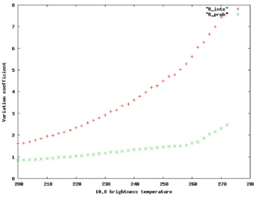
Assuming a sufficient database size, an empirical relation can be computed between infrared brightness temperatures and rainfall intensities. Using a ground radar network, Vi-cente et al. (1998) fit an exponential model through a loga-rithmic transformation. However this method raises the is-sue of the variance estimation error which is important for high precipitation rates. A way to mitigate this effect is to carry out the estimation on rainfall probability and not on rainfall intensity. On Fig. 1a the empirical relation between rain intensity and rainfall probability versus 10.8 µm temper-ature is displayed with a logarithmic scale. The computa-tions have been carried out on the 2006 whole African area and, for sampling and significance considerations, only the interval 200 K–273 K has been considered. In this interval, the shapes of these two curves look very similar and are con-sistent with an exponential model for a temperature lower than 260 K. The corresponding coefficient of variation, ratio of the standard deviation by the mean is plotted in Fig. 1b. This non-dimensional coefficient allows to compare the sig-nal to noise ratio of statistical relation. In the full range of temperature the coefficient of variation associated with the rainfall intensity is always greater than the probability
coef-Figure 1.b. Variation coefficient for the rainfall intensity (red curve) and the rainfall probability (green curve) versus 10.8 µm brightness temperature.
Fig. 1b. Variation coefficient for the rainfall intensity (red curve)
and the rainfall probability (green curve) versus 10.8 µm brightness temperature.
ficient and the minimal value of these two coefficient ratios is close to 2. This feature suggests that, in our database, the estimation of rainfall probability from cloud temperatures is much less noisy than for precipitation intensity.
Therefore the estimation is split in three steps: the pro-duction of a rainfall probability based on IR channels, the estimation of rainfall potential intensities by a downscaling process and the production of the accumulated rainfall. The rainfall potential intensity is a mean precipitation intensity conditioned by rain probability. Should the implementation use only one reference dataset for rainfall intensity the last step is straightforward. Otherwise the various potential in-tensity fields have to be merged. In an algorithm very similar to GPCP, the merging is then dependent on estimation vari-ance. This last part of the algorithm will not be developed in this paper.
4 Input data selection
To implement this global frame the first step is the selection of an input predictor set. The predictors selection is deeply dependent on the observation system and on the study area, and this part describes the algorithm implemented for the AMMA experiment. These predictors are selected from the 12 visible and infrared channels of the SEVIRI radiometer on-board MSG.
The 10.8 µm channel is used as a first order temperature factor. Located in a spectral window, its brightness tempera-ture allows for a direct retrieval of cloud top altitude. More-over all the meteorological satellite infrared sensors offered measurements in this wavelength and it was the base of the first results on satellite rainfall estimation (Arkin, 1979).
Figure 2.a. Difference of the mean value of 08.7 µm and 12.0 µm channels between non rainy and rainy pixels plotted versus 10.8 µm brightness temperature in red and green respectively. Curves are plotted with error-bars. Both scales are in Kelvin.
Fig. 2a. Difference of the mean value of 08.7 µm and 12.0 µm
channels between non rainy and rainy pixels plotted versus 10.8 µm brightness temperature in red and green respectively. Curves are plotted with error-bars. Both scales are in Kelvin.
At a first glance integrating information about solar backscattering radiation should enhance rainfall probability estimation. However the discontinuity between day and night should introduce a bias at the level of the diurnal cycle. As the temporal integration of validation data is scarcely shorter than one day correcting this bias should be a sensitive issue. Thus the three channels at 0.6 µm, 0.8 µm and 1.6 µm have not been selected. The 3.9 µm channel has been discarded also because of the different type of information provided during day and night-time, and of highly reflective back-ground problems due to sun glint, bare soils or deserts. More-over this channel accuracy is poor More-over cold clouds and thus it should introduce extra-noise in the statistical estimation.
SEVIRI integrates two split window channels: 8.7 µm and 12.0 µm. The 12.0 µm channel, primarily designed on the Tiros-N series, for sea surface temperature retrieval has demonstrated its efficiency for nephanalysis. It can help in discriminating semi-transparent cirrus as their brigthness temperature should be lower for 12.0 µm than for 10.8 µm (Derrien et al., 1993). It has been used by Inoue (1987) as an input for a statistical rainfall assessment. The 8.7 µm chan-nel can be used in association with 10.8 µm for high altitude cirrus screening (Schmetz et al., 2002). Moreover it adds facilities to identify cloud phase (Wolters et al., 2008).
As a first assessment of the split window channels effi-ciency, the whole dataset has been split in rainy and non rainy pixels according to TRMM/PR. For each subset the mean brightness temperature for the 8.7 µm and the 12.0 µm channel has been computed, then the difference of these two mean temperatures has been plotted versus the 10.8 µm tem-perature in Fig. 2a. The red curve represents the 8.7 µm channel and the green the 12.0 µm. The effects are oppo-site but these two curves show similar patterns. When
con-Figure 2.b. Difference of the mean value of 6.2 µm and 7.3 µm channels between non rainy and rainy pixels plotted versus 10.8 µm brightness temperature in red and green respectively. Curves are plotted with error-bars. Both scales are in Kelvin.
Fig. 2b. Difference of the mean value of 6.2 µm and 7.3 µm channels
between non rainy and rainy pixels plotted versus 10.8 µm bright-ness temperature in red and green, respectively. Curves are plotted with error-bars. Both scales are in Kelvin.
Figure 2.c. Difference of the mean value of 9.7 µm and 13.4 µm channels between non rainy and rainy pixels plotted versus 10.8 µm brightness temperature in red and green respectively. Curves are plotted with error-bars. Both scales are in Kelvin.
Fig. 2c. Difference of the mean value of 9.7 µm and 13.4 µm
chan-nels between non rainy and rainy pixels plotted versus 10.8 µm brightness temperature in red and green respectively. Curves are plotted with error-bars. Both scales are in Kelvin.
sidering the 8.7 µm (resp. 12.0 µm), on the whole range of 10.8 µm temperatures the mean value for rainy pixels is al-ways smaller (resp. greater) than for non rainy ones. The maxima of these curves indicate the area of best discrimi-nation efficiency. Note that these maxima area are slightly shifted, the 8.7 µm discriminating better at lower tempera-tures than the 12.0 µm.
The first water vapor channel has been introduced on Tiros-2 in 1960 to provide information about water vapor content. Two SEVIRI channels are located inside of the wa-ter vapor absorption band: 6.2 µm and 7.3 µm. In a mean
tropical atmosphere the peaks of their weighting functions are at 350 hpa and 500 hpa. Although these channels have been designed to measure water vapor content at different levels they also contain information about cloud height (Nie-man et al., 1993). Moreover, the difference between these two channels, correlated with water vapor content at the at-mosphere higher levels, can be interpreted as a cloud pre-cipitable water content (Schmetz et al., 2002). A complete description of these two channels can be found in (Santurette and Georgiev, 2005).
Figure 2b is similar to Fig. 2a; the difference for the 6.2 µm channel is plotted in red and for the 7.3 µm channel in green. Due to the low layers absorption the higher temperatures are not significant. Elsewhere they display the same trend, con-tinuously growing from 200 K until 255 K. In this interval the order of magnitude of the difference is almost twice as much as for the split-window channels.
The 9.7 µm channel belongs to the ozone absorption line; it offers facilities to evaluate the content of this component. But it can also be combined with other channels to evalu-ate the height of clouds and the air mass temperature (Kerk-mann et al., 2005; Lattanzio et al., 2006). In a similar way the 13.4 µm channel has been primarily designed for CO2
content observation. The difference between 13.4 µm and 10.8 µm channels can be used to discriminate convective cells from other clouds. Eyre and Menzel (1989) demonstrated that the combination of 13.4 µm and 11.1 µm channels of NOAA-7 satellite can be used in order to estimate cloud-top pressure which is highly correlated with altitude. It is particularly efficient to evaluate mid-level cloud heights. An important characteristic of these two channels is that the peak of their weighting function is lower than those of water va-por channels. In the same conditions as above, the maximum of CO2channel is obtained at 830 hpa and the maximum of
ozone channel at the ground pressure. Thus they can supply a complementary information in the troposphere lower layers. Figure 2c displays the difference graph for channels 8.7 µm (red) and 13.4 µm (green). Once again the differ-ence sign is constant on the whole temperature interval but the behavior of these two curves is rather different. Whereas the red curve has a clear maximum around 250 K, the green curve is almost flat. This feature should suggest that each channel has some capacity to filter non rainy events but the underlying phenomena are different.
Because of their relationship with cloud properties, all the SEVIRI thermal infrared channels (6.2 µm, 7.3 µm, 8.7 µm, 9.7 µm, 10.8 µm, 12.0 µm, and 13.4 µm) are selected as in-put predictors. All these channels are highly correlated to a general temperature factor. It has to be underlined that multi-spectral thermal properties act as a second order effect against this factor. To improve the convergence efficiency, one of the channels is chosen as reference and as first in-put and the differences between this channel and the others are considered as inputs for the neural network. The use of these differences can be considered as a naive
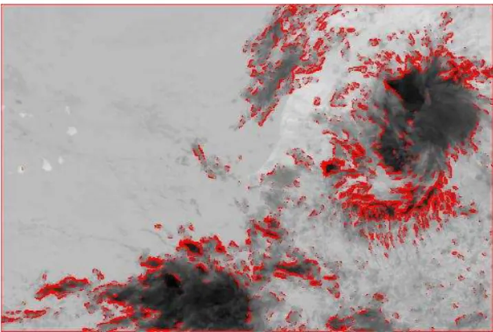
orthogonaliza-Figure 3. The 5% highest local variance values are plotted in red on the 8.7 µm channel image (20°N-11°N/26°W-12°W). The local variance has been computed on a 3x3 window.
Fig. 3. The 5% highest local variance values are plotted in red on
the 8.7 µm channel image (20◦N–11◦N/26◦W–12◦W). The local variance has been computed on a 3×3 window.
tion process between the global temperature factor and each thermal infrared channel. The choice of the reference chan-nel does not influence the learning process of the neural net-work. As mentioned above, the 10.8 µm channel is selected as a main temperature factor.
A local variance indicator of the 10.8 µm channel is of-ten used in order to discriminate convective cells from non rainy clouds (Adler and Negri, 1988; Jobard and Desbois, 1992). Underlying hypothesis is that top of clouds limited by an inversion layer would look flat whereas deep convec-tion should be associated with a non-uniform cloud top tem-perature. A local variance or a slope are currently used as an input for rainfall estimation models, but the actual effi-ciency appears as moderate (Ba and Gruber, 2000). As a matter of fact the high variance values are mainly associated with cloud boundaries (Fig. 3) because of the contrast with the ground. In some extent, this feature is related to rainfall as the more active cells are generated in the front of convec-tive systems, but the relation is still very indirect. In order to overcome partially this effect, other information have been chosen as inputs in the neural network. Both local variance of 10.8 µm thermal IR channel and of 6.2 µm water vapor chan-nel are used. The absorption by water vapor in this chanchan-nel is very high so that the surface and the lower layers of the at-mosphere are totally masked, reducing the contrast of cloud edges. Also, the maximum temperature value in the 5 pixel
×5 pixel window is selected in order to discriminate high values of spatial variance due to the contrast between clouds and ground (or high and low clouds) and those due to convec-tive cells. Moreover, both local variance of 10.8 µm thermal IR channel and of 6.2 µm water vapor channel are used.
In the life cycle of a convective cell the maximum of pre-cipitation occurs during the growing phase (Redelsperger, 1997). This time evolution is represented by a cooling index, difference between two successive 10.8 µm images. Among
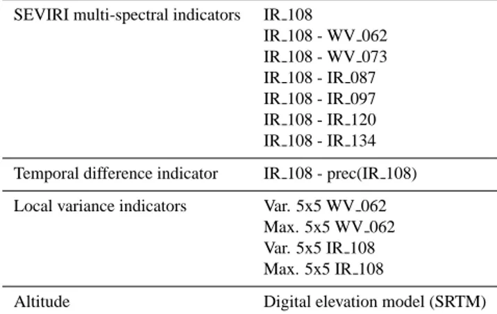
Table 1. Neural network input list. The SEVIRI channels are
de-noted following the Eumetcast standard (i.e. IR 108 means infrared 10.8 µm).
SEVIRI multi-spectral indicators IR 108
IR 108 - WV 062 IR 108 - WV 073 IR 108 - IR 087 IR 108 - IR 097 IR 108 - IR 120 IR 108 - IR 134 Temporal difference indicator IR 108 - prec(IR 108) Local variance indicators Var. 5x5 WV 062
Max. 5x5 WV 062 Var. 5x5 IR 108 Max. 5x5 IR 108
Altitude Digital elevation model (SRTM)
other factors, a decrease of the local brightness temperature may be related to a convective cloud expansion phase and then to higher probabilities of rainfall while an increase of the local brightness temperature may correspond to a con-vective cloud dissipation phase and to lower probabilities of rainfall.
Orographic effects can produce rainy events with specific patterns. In order to take into account this phenomenon, the altitude information is selected as an input. Altitude data are extracted from the digital elevation model based on the Shuttle Radar Topography Mission (SRTM).
The selected predictors are summarized in Table 1. In some extent this set has some redundancy and the estimation procedure has to cope with this feature. But the important fact is that each input is related to rainfall and does not intro-duce significant noise.
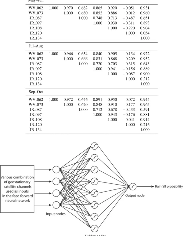
As far as a statistical process is involved, a Principal Com-ponent Analysis (PCA) could be used to reduce the number of input predictors. This preliminary transformation would both enhance the computation speed and the results stabil-ity. But the PCA relies on linear correlation relevance and in order to assess its liability correlation coefficients have been computed with different stratifications. In Table 2a, correla-tion matrices computed according to a two months temporal stratification are displayed. These matrices are computed on the seven SEVIRI channels from 6.2 µm to 13.4 µm for the whole African continent. At a first glance, these results look consistent, both signs and magnitude of correlation coeffi-cients are conserved among these three matrices. However this is a global feature which should be significant if precipi-tation were highly correlated with this main trend. A second stratification, based on a temperature threshold, has been in-troduced. Computation has been carried out on the same area from May to October 2006. The first matrix has been com-puted without any filtering and is therefore very similar to
the previous one. For the second, a 273 K threshold has been applied eliminating almost all direct ground signal and for the third matrix the threshold has been set to 233 K in order to focus on convective processes. The discrepancy between these three matrices appears clearly (Table 2b). Even if only atmospheric phenomena are considered no regular patterns are observed and the extracted PCA factors would be highly dependent on the selected threshold. Replacing the predic-tor set with the first PCA facpredic-tors would suppress some sig-nificant information for the low temperatures. It is a direct consequence of the the non linearity issue which has been previously mentioned.
5 Statistical procedure design
Estimating rainfall occurrence from this set of input predic-tors can be described as a non linear extension of a regres-sion analysis or a multidimenregres-sional extenregres-sion of histogram matching. Kiruno (1998) had to solve a similar problem when he designed an estimation process to retrieve precip-itation from three satellite channels. A discretization inter-val has been set on each component to compute a three-dimension table. This simple method estimates a precipi-tation rate for each node but is difficult to extend as the table size increases quickly with the predictors number and there-fore a stable estimation would require a huge learning set. By contrast a linear regression would produce a stable but also inaccurate result. The number of degrees of freedom highlights this difference. Let n be the number of input pre-dictors, the regression has n degrees of freedom whereas the multidimensional histogram matching hasQ
i=1,nlev(i)
de-grees of freedom where lev(i) is number of bins for the i-th predictor.
Feed forward neural networks appear as a compromise as their number of degrees of freedom is intermediate and de-pendent on the network architecture. Figure 4 is a graphical presentation of such a network. A set of hidden nodes acts as an intermediate between the predictors and the output of the network. The input of each hidden node is a linear combina-tion of the input predictors, this value is then transformed by an activation function. The network output itself is a linear combination of the hidden nodes output. Once the network architecture is designed, the linear combination coefficients have to be set in order to fit at best with the learning data set. The number of coefficients to estimate can be related to the degree of freedom of the model, in a feed forward network it is mn + m where m is the hidden nodes numbers. The universal approximation theorem (Hornik, 1991) states that such a network could approximate any continuous function with one hidden layer and a finite number of hidden nodes. The key point is that the activation functions are continuous and non linear; the sigmoid function has been selected for EPSAT-SG implementation.
Table 2a. Correlation matrices for three periods. May–Jun WV 062 1.000 0.970 0.682 0.865 0.920 −0.051 0.931 WV 073 1.000 0.680 0.852 0.886 0.012 0.960 IR 087 1.000 0.748 0.713 −0.487 0.651 IR 097 1.000 0.930 −0.311 0.893 IR 108 1.000 −0.220 0.904 IR 120 1.000 0.054 IR 134 1.000 Jul–Aug WV 062 1.000 0.966 0.654 0.840 0.905 0.134 0.922 WV 073 1.000 0.666 0.831 0.868 0.209 0.952 IR 087 1.000 0.720 0.703 −0.315 0.643 IR 097 1.000 0.941 −0.156 0.889 IR 108 1.000 −0.087 0.900 IR 120 1.000 0.212 IR 134 1.000 Sep–Oct WV 062 1.000 0.972 0.646 0.891 0.950 0.072 0.944 WV 073 1.000 0.620 0.848 0.910 0.177 0.965 IR 087 1.000 0.712 0.678 −0.433 0.591 IR 097 1.000 0.943 −0.176 0.881 IR 108 1.000 −0.041 0.914 IR 120 1.000 0.216 IR 134 1.000
Figure 4. Schematic representation of a feed forward neural network
Fig. 4. Schematic representation of a feed forward neural network.
Setting the number of hidden nodes is mainly an heuristic issue. It is usually presented as a trade-off between result accuracy versus network training time and error propagation due to truncated computer arithmetic. Moreover increasing
the number of hidden nodes could produce a network over-training. A comprehensive discussion on this topic can be found in Walczak and Cerpa (1999). Due to the learning set size, these side effects are unlikely to occur and the hidden
Table 2b. Correlation matrices computed with three different thresholds. Same layout as in Table 2a. 330 K WV 062 1.000 0.969 0.660 0.861 0.922 0.051 0.932 WV 073 1.000 0.655 0.841 0.885 0.130 0.959 IR 087 1.000 0.727 0.697 −0.417 0.627 IR 097 1.000 0.937 −0.223 0.884 IR 108 1.000 −0.120 0.904 IR 120 1.000 0.160 IR 134 1.000 273 K WV 062 1.000 0.958 0.262 0.841 0.909 0.384 0.914 WV 073 1.000 0.188 0.770 0.835 0.493 0.942 IR 087 1.000 0.605 0.478 −0.546 0.070 IR 097 1.000 0.965 0.033 0.748 IR 108 1.000 0.178 0.824 IR 120 1.000 0.615 IR 134 1.000 233 K WV 062 1.000 0.891 −0.377 0.741 0.845 0.568 0.847 WV 073 1.000 −0.218 0.703 0.770 0.482 0.778 IR 087 1.000 0.159 −0.022 −0.710 −0.464 IR 097 1.000 0.969 0.127 0.611 IR 108 1.000 0.285 0.722 IR 120 1.000 0.712 IR 134 1.000
Figure 5. RMSE is plotted against number of learning step iterations. Learning (resp. validation) dataset is plotted in plain (resp. dashed) line.
Fig. 5. RMSE is plotted against number of learning step iterations.
Learning (resp. validation) dataset is plotted in plain (resp. dashed) line.
nodes number is set to twice the input nodes number. The error back-propagation algorithm is perhaps the most widespread method to set the network coefficients
(Rumel-hart et al., 1986). After a random network initialization, each element of the training set is considered in a two-step com-putation. An error is computed by the difference between the network estimated value and the actual rainfall occurence value. Then this error, multiplied by a decaying impact co-efficient, is used to correct the network coefficient according to their relative importance in final output. This algorithm should converge on a local minimum of the error function provided it is repeated several times on the training set. As it is a step by step method the records order in the training set is not indifferent and the best results are obtained with a uni-form distribution error in this set. Therefore to suppress the correlation effect linked with remote sensing image coher-ence, a data scrambling where records are randomly ordered is performed before training.
To assess the reliability of the neural network chosen ar-chitecture, the co-located pixels dataset has been divided into two subsets: a learning database (75% of the cases) and a test database (25% of the cases). The first one is used to com-pute the coefficients values and the second one is dedicated to validate these coefficients with an independent dataset. The Root Mean Square Error (RMSE) between reference and es-timation is calculated for all iterations of the learning phase (Fig. 5). On this graphic, the two curves are similar even if the RMSE is slightly higher for the independent validation
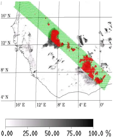
Fifure 6. EPSAT-SG rainfall probability estimate (gray scale) collocated with TRMM/PR
Fig. 6. EPSAT-SG rainfall probability estimate (gray scale)
collo-cated with TRMM/PR.
dataset. The second relevant information on this graphic is that the RMSE does not increase even after 500 learning iter-ations suggesting that there is no over-training effect and that the neural network is properly sized. As the RMSE decreases very slowly after 200 iterations, there is no interest in using more iterations. Finally, the RMSE for the learning dataset is about 18.25% and only 0.10% higher for the validation one. This RMSE value represents the uncertainty of the rainfall probability mean value.
Applying the resulting neural network coefficients to every MSG pixels of the studied area, instantaneous rainfall prob-ability images are provided with the MSG time and space resolutions. In Fig. 6 an estimated rainfall probability field (in gray tones) is superimposed with a coincident TRMM/PR track where rainy pixels are plotted in red and non-rainy in green. The active cells appear as clearly delineated by the rainfall probabilities. On this situation the main features of the precipitation field as detected by TRMM/PR are properly reproduced by the neural network output.
In order to assess to which extent the estimated rainfall probability is environment specific, four learning sets have been extracted on the AMMA area for 2004 and 2006. Two monsoon pre-onset datasets from 1 May to 30 June and two monsoon post-onset datasets from the 15 July to 15 Septem-ber. On each learning set a neural model has been fitted with
Table 3. Neural network estimation errors on different dataset (columns) versus training set (rows).
2004-mj 2004-jas 2006-mj 2006-jas 2004-mj 0.002889 0.004416 0.003016 0.004986 2004-jas 0.002895 0.004342 0.003027 0.004923 2006-mj 0.002957 0.004518 0.002975 0.005012 2006-jas 0.002995 0.004421 0.002964 0.004871
22 hidden nodes, then the mean quadratic error of this model has been computed for all the learning sets. The results are summarized in Table 3 where the lines are indexed by the estimated models and the columns by the learning sets. The interpretation of the matrix diagonal is slightly different as it represents a model bias and not an estimation bias. Nev-ertheless the results look as consistent: the values are more homogeneous among columns than among lines. This should suggest that an estimated network shows very similar perfor-mances on different periods and there is no real benefit to expect in retraining the network once is has been estimated on a significant dataset. The main error should be much more dependent on the meteorological phenomena distribu-tion which could explain the inter columns variadistribu-tion. It can be noticed that the columns smaller values are, except one, on the main diagonal. As expected the method performs better when using actual data rather than a previous estimation, but this advantage is minor and in one situation the estimation local minimum has been out performed by an other model.
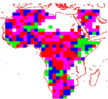
As suggested by these results, the relationship between in-frared brightness temperatures and precipitation cannot be improved by a simple temporal or spatial stratification. This hypothesis is confirmed by the classification carried out on the global dataset. This dataset has been split in two peri-ods (May to July and August to October) and according to a 2.5◦regular grid. On each box an empirical rainfall prob-ability function is computed. For a statistical stprob-ability rea-son only one channel (10.8 µm) is considered and the boxes with less than 3000 rainfall detections are discarded. Then a non-supervised classification in four clusters is performed for each period. This classification is based on a K-means algorithm: a number of clusters is set, then an iterative pro-cess splits the dataset in oder to minimize the intra-cluster variances. The variance computation relies on a simple Eu-clidian distance . This classification is purely statistical and does not integrate any input based on aerologic parameters, nevertheless it could be expected that some of the main cli-matic zones would match with generated classes. Figure 7a (resp. 8a) displays the four class centers and Fig. 7b (resp. 8b) the spatial class repartition. At a first glance the center class distribution are differentiated by their kurtosis, from a quasi linear relation (green curve) to a relation looking as a power law (purple curve). But even these two classes do not show any regularity in their spatial distribution and are
Figure 7.a. Pre-onset period: mean probability function for classes 0, 1, 2, 3. Temperature is coded in degree C.
Fig. 7a. Pre-onset period: mean probability function for classes 0,
1, 2, 3. Temperature is coded in degree C.
deeply different from one period to an other. None of the syn-optic scale atmospheric phenomena or agro-climatic zones can be identified on the classifications. The only identifiable pattern is the quasi-linear class (green code) which is in some extent associated with mountainous area. Precipitation en-hancement linked with relief and elevation is well known but this observation is slightly different: when orographic effects are predominant, cloudiness could not be used as a proxy for rainfall as the empirical relationship itself appears as orogra-phy dependent. But despite this local effect which should be confirmed by further studies, these observations suggest that using these boxes as a stratification basis would not enhance the estimation sensitivity but would only reduce the sample size.
6 Rainfall potential intensity
As written in Sect. 3, the EPSAT-SG rainfall estimate (REst)
is the product of the Rainfall Probabilities (RProb), by rainfall
potential intensity (RPotInt)maps:
REst=RProbxRpotint (1)
where REst, RProb and RPotIntare functions defined in space
and time.
The rainfall potential intensity (noted RPI below) is esti-mated by a downscaling method which is a way to include small scale variability extracted from geostationary sensors. The Rainfall Probability can be computed with the time and space resolution of GEO satellite which is far smaller than the statistical validity scale of any rainfall estimation prod-uct. But assuming selection of a rainfall reference product
Figure 7.b. Pre-onset period: Spatial repartition of the four classes computed by non supervised classification. Same color code as in Fig. 7.a.
Fig. 7b. Pre-onset period: Spatial repartition of the four classes
computed by non supervised classification. Same color code as in Fig. 7a.
and an associated space-time validity domain size , RPI can be estimated by the formula:
RPotInt(B) = ∫ B
Rref/∫ B
RProb (2)
where B is a spatio-temporal domain whose sizing is im-portant for final product accuracy and Rref an accumulated
rainfall field which is intermittent and/or defined at a coarser scale. It has to be noticed that B is not necessarily a regular box and should the rainfall reference be extracted from LEO microwave data, B would be a time buffer around the satel-lite swath inside a surrounding box. The issue is to derive RPI at the fine satellite resolution scale from RPI on the inte-gration domain B. A simple non overlapping set of domains could be considered and a RPI constant value computed for each element of this set. But such a process would produce rough boundary effect when downscaling. To avoid this ef-fect, B will be defined as a three-dimensional slide window. The Eq. (2) is then used to compute RPI on the center of the box which is defined as identical to RPotInt(B).
Setting the size of this slide window is mainly a statistical issue, the larger this size the greater the influence of rainfall probability field. Obviously a window size identical to the resolution of RPotIntwould produce a REstfield identical to
Rreffield. For the implementation of EPSAT-SG in AMMA
database, some operational considerations have lead to se-lect the GPCP product as the reference accumulated rainfall field. The window size has been set according to Richard and Arkin (1981) which state that the maximum of corre-lation between cold cloud duration and precipitation occurs for a window of one month by 2.5◦in latitude and longitude.
Figure 8.a. Post-onset period: mean probability function for class 0, 1, 2 and 3. Although this classification is independent from the previous one, color code is selected to get maximum similarity with Fig. 7.a. Temperature is coded in degree C.
Fig. 8a. Post-onset period: mean probability function for class 0,
1, 2 and 3. Although this classification is independent from the previous one, color code is selected to get maximum similarity with Fig. 7a. Temperature is coded in degree C.
This choice is conservative and a more sophisticated imple-mentation would have to deal with a window size which is dependent on an estimation error.
Among the GPCP products the daily 1◦grid has been ex-tracted and interpolated at the scale of the MSG pixel to con-stitute the Rreffields. The Eq. (3) is then the discrete
transla-tion of Eq. (2): RPotInt=α × P 31Days P 2.5deg res Rref ! P 31Days P 2.5deg res RProb ! (3)
where α is a correction coefficient set to counterbalance missing slots. From Eq. (3) a daily image of PRI is com-puted at the GEO satellite spatial resolution. According to this equation, RPotIntimages are the results of a 31-day
rain-fall accumulation (in millimeters) divided by a rainrain-fall dura-tion as expressed by the accumulated rainfall probability.
Equation (1) can be presented as an extension of the GPI (Arkin, 1979). But, whereas the rainfall probability part is only represented by a simple threshold, which provides 0% or 100% probabilities in the GPI method, the values of the rainfall probability maps calculated by the feed forward neu-ral network are varying from 0% to 100%. In a same way, the 3 mm/h rain rate value proposed by Arkin could be ap-plied, but the rainfall efficiency obviously is changing in ac-cordance with the geographic situation or the season. Rainy events on the Guinean Coast are much more frequent, but less intense than those which occur in the Sahelian region. Moreover, with the latitudinal gradient of humidity, the evap-oration phenomenon below clouds is more important in the
Figure 8.b. Post-onset period: Spatial repartition of the four classes computed by non supervised classification. Same color code as in Fig. 8.a.
Fig. 8b. Post-onset period: Spatial repartition of the four classes
computed by non supervised classification. Same color code as in Fig. 8a.
Sahelian region than close to the South coast. For all these reasons, it seems more appropriate to use a rainfall potential intensity value, which is varying in time and space, rather than a constant rain rate value.
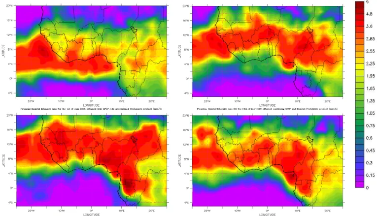
Figures 9 to 12 present four daily 2006 PRI images com-puted by different methods. The rain rates are expressed in millimeters per hour and it can be noticed that for all figures the PRI falls in a range of 0 to 6 mm/h. Those values are close to the GPI rain rate (3 mm/h). However, the fact that there is a maximum value of 6 mm/h is one of the limitations of the EPSAT-SG method: high precipitation rates and short-time rainfall events cannot be properly retrieved with this algo-rithm. This weakness is encountered in many methods based on geostationary satellite IR data. For some part it is linked to the low frequency of high intensity event and thus to the difficulty to retrieve them from a statistical process. But it can be mainly related to the indirect nature of the measure-ment. The neural network inputs are thermal infrared bright-ness temperatures and therefore inform about cloud canopy properties and not about intense precipitation location as in-dicated by radar data. The thermal infrared information ap-pears as smoothed compared with microwave information. In some extent the rainfall probability downscales the GPCP information but fails to render fine scale structures and thus attenuate the highest rainfall intensities.
Figure 10 is computed according to Eq. (3). A sliding space window is applied with a shift of one MSG pixel. Each obtained value of the right side of the Eq. (3) is set to the cen-tral position of the 2.5 degrees integration area. Therefore the integration zone is a disc of 42 pixels radius corresponding nearly to a 2.5 degrees diameter. Then, the sliding windows
(a) 1st of June
(b) 10th of July
(c) 20th of August
(d) 30th of September
Figure 9:
Rainfall potential intensity maps computed without spatial integration window
(a) 1st of June
(b) 10th of July
(c) 20th of August
(d) 30th of September
Figure 9:
Rainfall potential intensity maps computed without spatial integration window
(a) 1st of June (b) 10th of July
(c) 20th of August (d) 30th of September
Figure 9:
Rainfall potential intensity maps computed without spatial integration window
(a) 1st of June
(b) 10th of July
(c) 20th of August
(d) 30th of September
Figure 9:
Rainfall potential intensity maps computed without spatial integration window
(a) 1st of June
(b) 10th of July
(c) 20th of August
(d) 30th of September
Figure 9:
Rainfall potential intensity maps computed without spatial integration window
Fig. 9. Rainfall potential intensity maps computed without spatial integration window.
are applied in time and space and the final RPI products are provided with the time resolution of the reference dataset (1 day with GPCP-1dd) and the space resolution of the geosta-tionary satellite (3 km for MSG). On the contrary Fig. 9 is computed without spatial integration. A comparison of these two figures demonstrates clearly the benefits of using a spa-tial integration area. On one hand the artifacts created by 1◦ grid boundaries disappear. On the other hand some physi-cal discontinuities are better delineated. On the 1 June 2006 the Guinean shoreline effect appears more clearly in Fig. 10a than in Fig. 9a.
The Inter Tropical Convergence Zone (ITCZ) evolution can be clearly observed consistently with the season: on Fig. 10a the largest values are located over ocean just on south of the Guinean coast and these values are going north-ward during the rainy season (July and August) before going back southward in September.
Integrating this method in an operational environment raises the issue of producing a temporary rainfall estimator if the GPCP data are not available in due-time. In order to assess the impact of using a climatology instead of actual data, Fig. 11 is computed replacing 2006 GPCP data with an 8-year climatology (1997 to 2005).
When comparing Fig. 10 and Fig. 11, similar patterns ap-pear with very comparable values. There is an exception con-cerning the 30 September 2006 (Figs. 10d and 11d). This dif-ference is due to a very late rainy season over West Africa in 2006, which cannot be satisfactorily reflected by the clima-tology. But the values remain stable with a maximum close to 6 mm/h. Anyway the rainfall probabilities correspond to the 2006 rainy season situation and cloud trajectories and not to the climatology. This feature makes the images presented on Fig. 11 patchier than those on Fig. 10. Although inte-grating directly a rainfall climatology could produce some provisional results it appears much more appropriate to use a PRI climatology computed on coincident rainfall probabil-ities and rainfall reference intensprobabil-ities.
An other way to reduce the product delivery delay would be to select a reference rainfall data-source based on passive microwave from LEO satellites. Contrary to the GPCP which is highly dependent on rain-gauges data, this data-source is available in near real-time. To test this alternative a PRI (Fig. 12) is computed from the 3B42 product which is mainly calibrated by passive microwave data.
Several remarks arise from the comparison between Figs. 10 and 12. First of all, RPI have again the same range from 0 to 6 mm/h which reinforces the idea of stability of this
(a) 1st of June
(b) 10th of July
(c) 20th of August
(d) 30th of September
Figure 10. EPSAT-SG daily Rainfall Potential Intensity.
(a) 1st of June
(b) 10th of July
(c) 20th of August
(d) 30th of September
Figure 10. EPSAT-SG daily Rainfall Potential Intensity.
(a) 1st of June (b) 10th of July
(c) 20th of August (d) 30th of September
Figure 10. EPSAT-SG daily Rainfall Potential Intensity.
(a) 1st of June
(b) 10th of July
(c) 20th of August
(d) 30th of September
Figure 10. EPSAT-SG daily Rainfall Potential Intensity.
(a) 1st of June
(b) 10th of July
(c) 20th of August
(d) 30th of September
Figure 10. EPSAT-SG daily Rainfall Potential Intensity.
Fig. 10. EPSAT-SG daily rainfall potential intensity.
product. Moreover, the RPI values are still increasing in the ITCZ and large climatic regions have more or less the same values. However, if the RPI were very smooth with GPCP-1dd they are not with 3B42. This is due to the nature of the respective reference datasets. The GPCP-1dd estimates are conditioned by geostationary information and ground net-work which deliver time continuous data series. By contrast the 3B42 estimator depends highly on the LEO satellite cov-erage and is greatly influenced by the microwave estimated rain rates used as input. The related risk is to overestimate locally rainfall estimates causing the apparition of high value spots on RPI maps. The spot positions depend on the co-localization of LEO satellite data and rainy events during the period of study, which is unpredictable. The simple inte-gration frame proposed for AMMA implementation appears as more adapted to GPCP than to 3B42. Integrating a mi-crowave only product should likely require a more complex sliding window design associated to an along track product rather than to a gridded product. But this should also make the implementation much more complex.
7 Estimated rainfall
A Rainfall Probability Intensity (RPotint)can be interpreted
as the mean rate of a daily rain event and a Rainfall
Proba-bility (RProb)as the duration of this event. As a single RPI
is computed for the AMMA implementation, computation of accumulated rainfall is rather straightforward. Once the RPI maps are computed, the estimated rainfall estimates (REst)
can be obtained with the space and time resolution of MSG. At time t during day d and pixel a the REst value can be
derived from Eq. (1) as follows:
REst(a,t ) = RProb(a,t ) × RPotInt(a,d) (4)
Rainfall estimates are obtained with MSG time and space resolution. However, as this method is mainly based on geo-stationary satellite data, final estimates have to be integrated in time and space in order to limit the estimation bias. The principal interest of this fine time and space resolution is its flexibility for the users. It can be integrated in time and space to fit with products of any other scales or boundaries like a daily period starting at 6 a.m. or like a specific watershed.
The estimated rainfall accumulation during a period T can be easily computed by the following formula:
REst(a,T ) = 1 α X t ˆI T REst(a,t ) (5)
where the coefficient α is the same the one in Eq. (3). Indeed, the fact that there are missing probability images leads to an
(a) 1st of June
(b) 10th of July
(c ) 20th of August
(d) 30th of September
Figure 11. EPSAT-SG Rainfall Potential Intensity computed with a 8-year climatology instead of
actual data.
(a) 1st of June
(b) 10th of July
(c ) 20th of August
(d) 30th of September
Figure 11. EPSAT-SG Rainfall Potential Intensity computed with a 8-year climatology instead of
actual data.
(a) 1st of June (b) 10th of July
(c ) 20th of August (d) 30th of September
Figure 11. EPSAT-SG Rainfall Potential Intensity computed with a 8-year climatology instead of actual data.
(a) 1st of June
(b) 10th of July
(c ) 20th of August
(d) 30th of September
Figure 11. EPSAT-SG Rainfall Potential Intensity computed with a 8-year climatology instead of
actual data.
(a) 1st of June
(b) 10th of July
(c ) 20th of August
(d) 30th of September
Figure 11. EPSAT-SG Rainfall Potential Intensity computed with a 8-year climatology instead of
actual data.
Fig. 11. EPSAT-SG rainfall potential intensity computed with a 8-year climatology instead of actual data.
underestimation of rainfall amounts and a correction coeffi-cient is necessary to extend the total rainfall amounts to the whole studied period T .
Figure 13 represents EPSAT-SG (Fig. 13a) and GPCP-1dd (Fig. 13b) rainfall accumulation estimates for the 10 July 2006. High rainfall patterns can be seen on the west coast of Guinea and Sierra Leone, over the border between Burk-ina and Mali and over South Chad. North of 14◦N, rainy events are quite inexistent which is in accordance with the Sahelian climatology. The maximum daily accumulated pre-cipitation of 40 mm is realistic too. The fine structure of convective clouds is clearly apparent on Fig. 13a. Most of the patterns can be observed on both images. More details can be observed on EPSAT-SG estimates and they are also some differences such as the pattern seen over East-Mali. As the only available ground data are the synoptic stations dis-tributed through the Global Telecommunication System it is difficult to assess the relative accuracy of these two products. Two synoptic stations, Nara and Nioro-Sahel, are located on the area of the raining spot detected by EPSAT-SG but none of these two stations reported any data. The only ground in-formation can be extracted from Mauritanian Nema station which is on the periphery of this spot. The reported 24 h ac-cumulation of 5 mm on the 11 July 2006 morning should be more consistent with EPSAT-SG estimation than with
GPCP-1dd. The discussion highlights the difficulty of fine product inter-comparison based on scarce network.
When the EPSAT-SG estimates are gridded by 1◦ to fit with the GPCP space resolution (Fig. 13c) some lower values of the rainfall amounts can be observed when compared with the GPCP estimates on Fig. 13b. This is due to the smooth-ing effect induced by the downscalsmooth-ing formula presented in Eq. (2). It can be noticed that the main differences occur in coastal and mountainous area where the spatial gradient of precipitation is strong and therefore the smoothed gridded precipitation fields are inaccurate.
To point the differences between rainfall probability and rainfall estimation products, both of them have been repre-sented. Figure 14a shows the mean rainfall probability dur-ing August 2006 and Fig. 14b corresponds to the rainfall amount during the same period. These two images contain similar patterns as it could be expected from the method con-cept. This similarity can be observed around the west coast. However, there are some differences over Guinea and Nigeria where rain accumulations are higher than it could be antic-ipated from the rainfall probability. On the contrary, above 16◦N, rainfall accumulations seem to be less important than expected.
(a) 1st of June
(b) 10th of July
(c) 20th of August
(d) 30th of September
Figure 12. EPSAT-SG daily Rainfall Potential Intensity maps computed with 3B42 product instead of
GPCP-1dd.
(a) 1st of June
(b) 10th of July
(c) 20th of August
(d) 30th of September
Figure 12. EPSAT-SG daily Rainfall Potential Intensity maps computed with 3B42 product instead of
GPCP-1dd.
(a) 1st of June (b) 10th of July
(c) 20th of August (d) 30th of September
Figure 12. EPSAT-SG daily Rainfall Potential Intensity maps computed with 3B42 product instead of GPCP-1dd.
(a) 1st of June
(b) 10th of July
(c) 20th of August
(d) 30th of September
Figure 12. EPSAT-SG daily Rainfall Potential Intensity maps computed with 3B42 product instead of
GPCP-1dd.
(a) 1st of June
(b) 10th of July
(c) 20th of August
(d) 30th of September
Figure 12. EPSAT-SG daily Rainfall Potential Intensity maps computed with 3B42 product instead of
GPCP-1dd.
Fig. 12. EPSAT-SG daily rainfall potential intensity maps computed with 3B42 product instead of GPCP-1dd.
Figure 13.a. Daily cumulated EPSAT-SG rainfall estimation. Fig. 13a. Daily cumulated EPSAT-SG rainfall estimation.
8 Validation
When validating a downscaling method a first issue is to as-sess the positive impact on the downscaled information itself. This validation exercise has been performed for the Sahelian
Figure 13.b. GPCP-1dd rainfall estimation
Fig. 13b. GPCP-1dd rainfall estimation.
region in West Africa during the 2004 rainy season. A rain-gauge network is managed by the CILSS organism (Comit´e permanent Inter-´etats de Lutte contre la S`echeresse au Sahel)
Figure 13.c. Daily cumulated EPSAT-SG on a 1° grid.
Fig. 13c. Daily cumulated EPSAT-SG on a 1◦grid.
Figure 14.a. EPSAT-SG rainfall probability field for August 2006
Fig. 14a. EPSAT-SG rainfall probability field for August 2006.
which concentrates data from nine different countries (Burk-ina Faso, Cap-Verde, Gambia, Guinea Bissau, Mali, Maurita-nia, Niger, Senegal and Chad). The data have been obtained from AGRHYMET as kriged fields on 10-day periods with 0.5 and 1 degree space resolution. The kriging method is described in Ali et al. (2005) and an associated estimation error of the rainfall amount is provided for each grid box. This network gathers about 645 stations including 75 synop-tic stations which transmit their data through GTS (Global Telecommunication System). Because GPCP integrates the GTS transmitted data in the product, the synoptic stations have been excluded from the computation of the kriged maps in order to guarantee the independence between estimation data and validation data. Figure 15 represents the CILSS area and the CILSS and synoptic rain-gauges positions.
Figure 14.b. EPSAT-SG accumulated rainfall field for August 2006
Fig. 14b. EPSAT-SG accumulated rainfall field for August 2006.
Figure 15. CILSS synoptic and climatic rain-gauges (Ali et al., 2005)Fig. 15. CILSS synoptic and climatic rain-gauges (Ali et al., 2005).
The statistical parameters used to validate these results are the Bias, the Root Mean Square Difference (RMSD), the Skill Score Index, and the explained variance, R2. The Bias represents the mean error produced by the algorithm accord-ing to the validation dataset while the RMSD is the average distance between estimation and its corresponding reference in a grid cell. The R2expresses the degree of agreement be-tween the estimated rainfall accumulation and the reference ones. The Skill Score Index is equal to 1 if estimation and reference match perfectly and is equal to 0 if the estimation is obtained by random distribution. The interest of the skill index is to deal with the assymetric distribution of the esti-mated variable.
Because of the spatial heterogeneity of the rain-gauge network managed by AGRHYMET, a first study has been performed during the 2004 rainy season in order to assess the effect on validation of grid cells having few or zero rain-gauges. Table 4 summarizes the validation statistic
Table 4. EPSAT-SG validation statistic parameters for three datasets with different minimum number of rain-gauges per grid-cell.
Bias rmsd R2 skill n.cells All cells 4.6 20.9 0.67 0.64 14 400 1 gauge 5.5 17.3 0.73 0.70 2787 2 gauges 4.8 17.2 0.73 0.71 899
parameters with best scores written in bold style, for the full dataset and two subsets. These subsets group only grid cells with a minimum of 1 or 2 embedded raingauges . The total number of grid cells is 14 400 but only less than 20% have at least one rain gauge, and about 6% have a minimum of 2 rain-gauges. The bias does change significantly when computed on grid cells with 0, 1 or 2 minimum raingauges. However it appears clearly that the RMSD, R2and Skill score index val-ues are improving when the minimum number of rain-gauges per grid cells increases. However it has been checked that the improvement is really small when the minimum number is 3 instead of 2.
To improve the reliability of this validation exercise, only grid cells with at least 1 rain-gauge are taken into account. This validation is done for 10-day periods, as validation data are only available at this time resolution. The comparison has been made with a space resolution of 0.5 degree in order to get enough grid cells to be statistically significant. So the GPCP-1dd has been interpolated to this final space resolu-tion.
The validation statistical parameters are presented in Ta-ble 5 for EPSAT-SG and GPCP-1dd; they have been com-puted on a set of 2787 grid cells containing at least one rain-gauge. EPSAT-SG estimates look better than GPCP-1dd for all the criteria. EPSAT-SG gets smaller RMSD value and higher R2(0.73) and Skill Score index value (0.79) than the GPCP-1dd reference dataset (respectively 0.57 and 0.42).
Scatter plots comparing GPCP-1dd or EPSAT-SG with rain-gauge kriged data are represented on Fig. 16. As it could be expected the regression line shows that the two products underestimate high precipitations and overestimate low ones. However the EPSAT-SG scatter plot (Fig. 16b) appears as more concentrated around the diagonal than the GPCP scat-ter plot (Fig. 16a). Even upscaled to match with the reso-lution of the rainfall reference product, EPSAT-SG performs better than GPCP-1dd. It is obvious that EPSAT-SG is bound to GPCP-1dd by construction; the correlation coefficient be-tween the two datasets in fact is 0.9 and their close relation-ship is illustrated by the scatter plot of Fig. 16c. Neverthe-less EPSAT-SG brings a sensible improvement. This result could look surprising but it demonstrates the interest of using a large enough slide window as already discussed in Sect. 6. A more complete validation comparing EPSAT-SG with other operational rainfall products can be found in Jobard et
Table 5. EPSAT-SG and GPCP-1dd validation statistic parameters
fot the AGRHYMET 10-day dataset with a minimum of one gauge per grid-cell.
Bias rmsd R2 skill EPSAT-SG 5.5 17.3 0.73 0.70 GPCP-1dd 6.0 24.0 0.57 0.42
al. (2010). The inter-comparison is carried out for ten rainfall estimation methods: three regional method specifically im-plemented on the West-African area (EPSAT-SG, TAMSAT and RFE.2), three global methods (GPCP-1dd, TRMM-3B42 and GSMAP MVK) and four real-time methods which are only satellite based (PERSIANN, 3B42-RT, CMORPH and GPI). This comparison is based on 10-day accumulated prod-ucts computed for three rainy seasons in West-Africa. The main trend is that global methods perform better than real-time ones and they are themselves outperformed by regional methods. Among the regional products, EPSAT-SG gets better results on most of statistical criteria although RFE.2 matches better the validation dataset considering distribution and bias.
Using three dense rain-gauge networks implemented for the AMMA experiment, Roca et al. (2010) developed an innovative approach to compare satellite estimation with ground data taking the various estimation errors into account. Whereas their results are consistent with the ones of Jobard et al. (2010) for 10-day periods, this is not true for shorter peri-ods. When retrieving the diurnal precipitation cycle, EPSAT-SG appears as less efficient than 3B42. Because of a strong thermal infrared contribution EPSAT-SG is sensitive to the lag between the active convection phase and the development of a stratiform tail. Some improvements can be expected by completing the predictor set by some parameters more closely related to the cloud dynamic. To enhance the diurnal phase estimation, Berg`es et al. (2009) proposed a cloud patch growing rate to be integrated as an input parameter.
9 Conclusion
EPSAT-SG, a rainfall estimation method, has been presented as a concept frame and its first implementation has been described and commented. The complexity of rainfall re-lated data collection system (satellites, radars and ground networks) compel a production procedure to match with the actual operational environment.
Every rainfall estimation procedure has to consider the weakness of the link between infrared signature and precipi-tation intensity. EPSAT-SG uses GEO data only for a Rain-fall Probability assessment. For the AMMA implementation these probabilities are estimated through a feed forward neu-ral network. The results appear as fairly good and suggest
Figure 16.a. Scatter-plot of GPCP-1dd versus validation rain-gauge dataset.Fig. 16a. Scatter-plot of GPCP-1dd versus validation rain-gauge dataset.
Figure 16.b. Scatter-plot of EPSAT-SG versus validation rain-gauge dataset.Fig. 16b. Scatter-plot of EPSAT-SG versus validation rain-gauge dataset.
an interesting stability property: once the network is trained, its coefficients could be applied to other time periods without significant loss of accuracy.
The rainfall potential intensity is a new concept introduced in EPSAT-SG. The idea beyond this conditional rainfall in-tensity is that it takes into account the local aerologic envi-ronment whereas the Rainfall Probability retrieves the sys-tem tracking information. In a simple case, as the AMMA implementation, it performs a downscaling of a rainfall ref-erence field. But it would also allow to merge various pre-cipitation intensity fields on the basis of their local estimation error.
Figure 16.c. Scatter-plot of EPSAT-SG versus GPCP-1dd.Fig. 16c. Scatter-plot of EPSAT-SG versus GPCP-1dd.
The Estimated Rainfall, which is the product of a Rainfall Probability and a rainfall potential intensity, is obtained at the fine resolution of the GEO satellite (3 km and 15 min for MSG) . Obviously associated errors should be important at this scale. But this resolution allows to match with any final product grid size or any watershed for hydrological models and crop models.
The comparison of EPSAT-SG with GPCP-1dd on the 2004 rainy season shows sensible accuracy improvements even when accumulating on 10-day periods. This result sug-gest that the downscaling procedure is running efficiently and reduces the error of the ingested rainfall product.
After the integration of EPSAT-SG products in AMMA database, a new implementation has been defined and in-stalled in AGRHYMET Center. This new version, designed to run both in near real time and in differed mode, is currently under evaluation. Moreover the described method can be easily extended to area covered by other GEO satellites than MSG. It can also be tuned to integrate other rainfall reference data sources than GPCP. In the frame of the future Megha-Tropiques operational products, the adaptation of EPSAT-SG is developed to ingest all the geostationary satellites covering the full tropical belt.
Acknowledgements. Based on a French initiative, AMMA was built
by an international scientific group and is currently funded by a large number of agencies, especially from France, the UK, the US and Africa. It has been the beneficiary of a major financial con-tribution from the European Community’s Sixth Framework Re-search Programme. Detailed information on scientific coordina-tion and funding is available on the AMMA Internacoordina-tional web site: http://www.amma-international.org.
Topical Editor F. D’Andrea thanks two anonymous referees for their help in evaluating this paper.