HAL Id: hal-02408975
https://hal.sorbonne-universite.fr/hal-02408975
Submitted on 13 Dec 2019
HAL is a multi-disciplinary open access
archive for the deposit and dissemination of
sci-entific research documents, whether they are
pub-lished or not. The documents may come from
teaching and research institutions in France or
abroad, or from public or private research centers.
L’archive ouverte pluridisciplinaire HAL, est
destinée au dépôt et à la diffusion de documents
scientifiques de niveau recherche, publiés ou non,
émanant des établissements d’enseignement et de
recherche français ou étrangers, des laboratoires
publics ou privés.
Annelid polychaetes experience metabolic acceleration
as other Lophotrochozoans: inferences on the life cycle
of Arenicola marina with a Dynamic Energy Budget
model
Lola de Cubber, Sebastien Lefebvre, Théo Lancelot, Lionel Denis, Sylvie
Marylène Gaudron
To cite this version:
Lola de Cubber, Sebastien Lefebvre, Théo Lancelot, Lionel Denis, Sylvie Marylène Gaudron. Annelid
polychaetes experience metabolic acceleration as other Lophotrochozoans: inferences on the life cycle
of Arenicola marina with a Dynamic Energy Budget model. Ecological Modelling, Elsevier, 2019, 411,
pp.108773. �10.1016/j.ecolmodel.2019.108773�. �hal-02408975�
Annelid polychaetes experience metabolic acceleration as other
1
Lophotrochozoans: inferences on the life cycle of Arenicola
2
marina with a Dynamic Energy Budget model
3
Lola De Cubbera,˚, Sébastien Lefebvrea, Théo Lancelota, Lionel Denisa, Sylvie Marylène
4
Gaudrona,b
5
aUniv. Lille, Univ. Littoral Côte d’Opale, CNRS, UMR 8187 Laboratoire d’Océanologie et de Géosciences, 62930
6
Wimereux, France
7
bSorbonne Univ., UFR 918 & UFR 927, 75005 Paris, France
8
Abstract 9
Arenicola marinais a polychaete (Lophotrochozoan) displaying a complex bentho-pelagic life
10
cycle with two larval dispersal phases, only partially described up to now. A Dynamic Energy
11
Budget (DEB) model was applied to the species in order to reconstruct its life cycle and growth
12
under in situ environmental conditions. Two types of DEB models are usually applied to other
13
Lophotrochozoans displaying similar life cycles: the standard (std-) model, applied to polychaetes
14
(5 entries among the 1524 of the Add-my-Pet database on the 18/10/2018), and the abj-model,
15
which includes an acceleration of metabolism between birth and metamorphosis, and which has
16
been applied to most molluscs (77 abj- entries out of the 80 mollusc entries) enabling better fit
17
predictions for the early life stages. The parameter estimation was performed with both models to
18
assess the suitability of an abj-model for A. marina. The zero-variate dataset consisted of length
19
and age data at different life cycle stages, the lifespan, the maximum observed length, and the wet
20
weight of an egg. The uni-variate dataset consisted of two growth experiments from the literature
21
at two food levels and several temperatures, laboratory data of oxygen consumption at several
22
temperatures, and fecundity for different lengths. The predictions of the abj-model fitted better to
23
the data (SMSE = 0.29). The acceleration coefficient was ca 11, which is similar to mollusc values.
24
The field growth curves and the scaled functional responses (as a proxy of food levels) were suitably
25
reconstructed with the new parameter set. The reconstruction of the early life-stages chronology
26
according to in situ environmental conditions of a temperate marine ecosystem indicated a first
27
dispersal phase of 5 days followed by a 7 months temporary settlement before a second dispersal
28
phase in spring, at the end of metamorphosis. We emphasize the need for using abj-models for
29
polychaetes in future studies.
30
Key words 31
Bioenergetics, lugworm, growth, oxygen consumption, life-history traits, dispersal
32
Introduction 33
Arenicola marina(Linnaeus, 1758) is a marine polychaete (Lophotrochozoan, Annelida)
inhab-34
iting most intertidal soft sediments from the Arctic to the Mediterranean. The species is intensively
35
dug for bait by recreational fishermen (Blake, 1979; De Cubber et al., 2018; Watson et al., 2017)
36
and the comparison between harvest efforts and observed populations abundance has evidenced
37
the need for some regulation of this activity in some places (De Cubber et al., 2018). In
aquacul-38
ture, A. marina is also reared for bait (Olive et al., 2006), and more recently, for its particular
39
haemoglobin that might represent a valuable blood substitute for humans in the future (Rousselot
40
et al., 2006) and which is already used for organs conservation before transplantation. However,
41
its complex bentho-pelagic life cycle with two dispersal phases before recruitment has made the
42
description of the early life stages and their chronology complicated, and still little is known about
43
the development of A. marina between the trochophore larva stage and the benthic recruitment
44
(Farke and Berghuis, 1979a, b; Newell, 1948; Reise, 1985). Moreover, the literature regarding A.
45
marina’s life cycle and growth is quite ancient (mostly from 1979) and since 1990, it has been found
46
that two cryptic species actually exist and might live in sympatry: A. marina and A. defodiens.
47
Therefore ancient life-history description has to be used with caution (Cadman and Nelson-Smith,
48
1990).
49
The ‘Dynamic Energy Budget’ (DEB) theory quantifies the energy allocation to growth and
50
reproduction of an individual during its life cycle according to environmental conditions such as
51
temperature and food availability (Kooijman, 2010) even in species with complex and numerous
52
life-stages (Llandres et al., 2015). Twelve primary parameters are sufficient for the implementation
53
of a standard (std-) DEB model. However, among the assumptions implied in std-DEB models,
54
some, like isomorphism during growth, the fact that growth always follows a typical Von Bertalanffy
55
growth curve, or the presence of three life stages (embryo, juvenile and adult) are not found in every
56
species. Therefore, extensions of the std-model (implying the use of more parameters) were created
57
(Kooijman, 2014) accounting for deviations from typical development implied by the std-model,
58
like foetal development, acceleration of metabolism, or extra life stages.
59
As of October 2018, Add-my-Pet (AmP) database estimated DEB parameters for 1524 animal
60
species (Marques at al., 2018). Among these entries, only 11 were annelid species, 4 of them being
61
polychaetes species for which std-models were applied. The closest phylum with a large amount
62
of data is the molluscs’ phylum (over 80 entries), also presenting a larval stage. Indeed, annelids
63
and molluscs belong to the Lophotrochozoan clade and both, after the embryogenesis, lead to a
64
trochophore larval stage. Mostly abj-DEB models have been applied only for the mollusc phylum,
65
which are an extension of std-models considering an acceleration of metabolism between birth (first
66
feeding) and metamorphosis (end of the change of shape) and are applied to most species with a
67
larval phase (Kooijman, 2014). Although polychaete species often present a larval phase during
68
their life cycle, until now, abj-models were not applied to this taxa.
A std- entry for A. marina is present in the AmP database and enables predictions of the
70
growth and reproduction of the species. However, more than half of the dataset used for the
71
parameter estimation consists of unpublished data (time since birth at puberty and maximum
72
reproduction rate taken from Marlin: https://www.marlin.ac.uk/ and lifespan and ultimate total
73
length taken from Wikipedia: https://www.wikipedia.org/), guessed data (wet weight at birth and
74
puberty, ultimate wet weight), or data related to other species (age at birth from A. cristata and
75
A. brasiliensis) (AmP entry: Bas Kooijman. 2015. AmP Arenicola marina, version 12/07/2015).
76
We therefore completed the data set with literature, experimental and field data, and implemented
77
a new parameter estimation for the species using both a std- and an abj-DEB models.
78
The objectives were:
79
(1) to calibrate a DEB model for A. marina based on a reliable and complete dataset and
80
adapted to its life cycle features (and therefore to compare the relevance of the use a std- or
81
an abj-DEB model for this species)
82
(2) to make predictions about the chronology of the early life stages of A. marina and the growth
83
potential according to the environmental conditions
84
(3) to compare the parameters of the DEB models implemented for A. marina with the other
85
Lophotrochozoan species’ parameters and discuss the advantages of the use of an abj-model
86
for this species.
87
1. Material and Methods 88
1.1. The DEB theory and its implementation for Arenicola marina
89
1.1.1. The model
90
The DEB theory describes the energy flows within an organism between three compartments
91
(state variables) : the reserve (E), the structure (V ), and the maturity (EH) or the reproduction
92
buffer (offsprings) (ER) according to its life stage in order to describe its energy allocation to
93
growth and reproduction for a given food level and at a reference temperature Tref (Fig. 1). The
94
three differential equations linked to the state variables are obtained from the expression of the
95
different fluxes (Table 1)(Kooijman, 2010; Van der Meer, 2006).
96
Temperature corrections are made to the rates considered by the model in the equation of
97
fluxes (e.g. the surface-area specific maximum assimilation rate, t 9pAmu(J.cm-2.d-1), the energy
98
conductance, 9v (cm.d-1), the specific volume-linked somatic maintenance rate, [ 9p
M] (J.cm-3.d-1),
99
and the maturity maintenance rate coefficient, 9kJ (d-1), see Tables 1 and 4). Indeed, when the
100
temperature T (K) is different from the reference temperature Tref (taken to be 293.15 K) these
101
rates are multiplied by the correction given in Equation (1), where TAis the Arrhenius temperature
102
(K), 9k1 the rate of interest at Tref and 9k the rate of interest at T .
103 9kpT q “ 9k1¨exp ˆ TA Tref ´TA T ˙ (1)
The links between observable metrics (physical length and wet weight) and the DEB model
104
quantities are made with the shape coefficient δ (varying between δ “ δM efor embryos and δ “ δM
105
after metamorphosis), the density of wet structure dV (g.cm-3), of wet reserve dE (g.cm-3) and of
106
dry reserve dEd(g.cm-3), the specific chemical potential of reserve µEd(J.Cmol´1of reserve), and
107
the molar weight of reserve wEd(g.Cmol´1) (Table 1). Here, we assumed that dV “ dE“1 g.cm-3,
108
dEd“0.16 g.cm-3, µEd“550000 J.Cmol´1 and that wEd“23.9 g.Cmol´1.
109
1.1.2. Adaptation to Arenicola marina’s life cycle
110
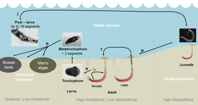
The spawning event of Arenicola marina happens in late summer or early autumn (De Cubber
111
et al., 2018; Watson et al., 2000). After the external fertilization, the embryo develops in the female
112
gallery up to the post-embryonic stage, the trochophore larva, which is able to move vertically in
113
the water column (Fig. 2, Farke and Berghuis, 1979a, b). At this time, the shape is changing
114
from ovoidal (oocytes, with a shape coefficient δ “ δM e) to cylindrical when the trochophore larva
115
gradually acquires new setiger becoming a metatrochophore larva (of shape coefficient δ ă δM e).
116
The metatrochophore larva is released in the water column when it reaches 3 setigers and is
117
transported by currents during several days. In lugworms, embryos and larvae are lecithotrophic,
118
living on maternal reserve and therefore supposed not to be able to feed (the maturity threshold
119
EH did not yet reach its value for birth: EH ă EbH, where birth is the time when individuals start
120
to feed). Therefore, there is no feeding or assimilation flux during the embryo and larval stage and
121
dE{dt “ ´ 9pC (Table 1). Moreover, these young stages do not have enough complexity yet to be
122
able to produce gametes and the reproduction flux goes to maturity (Table 1), which represents in
123
this case the acquisition of complexity of the individual (Fig. 1).
124
The metatrochophore larva settles and begins eating as post-larva, when the gut appears
func-125
tional (EH “ EHb), either on mussel beds, macroalgae or sheltered soft sediment bottoms (Fig.
126
2). At this point, it lives inside a mucus tube stuck to the bottom and feeds on the particles
127
deposited on the tube and around it, as well as on suspended particles (Farke and Berghuis, 1979a,
128
b; Newell, 1949; Reise, 1985; Reise et al., 2001). During this temporary settlement period, the
129
post-larva continues to gradually acquire new setigers up to the 19 final setigers found in adults
130
(the shape coefficient δ keeps on decreasing until it reaches the shape coefficient value of the adults
131
δM), developing a proboscis in the way of the adults (Farke and Berghuis, 1979a, b; Newell, 1949).
132
These morphological changes are assimilated to metamorphosis (up to when the maturity threshold
133
EH reaches its value at metamorphosis: EH “ EHj). During this period, a metabolic acceleration
134
(Kooijman, 2014) was considered, which is supposed to happen in most species that have a
lar-135
val phase, frequently coinciding with morphological metamorphosis (Marques et al., 2018), and
136
resulting in an exponential growth of the organism between the first feeding and the end of
meta-137
morphosis. From birth (EH“ EHb), feeding and assimilation are not null anymore, but individuals
138
are not able yet to produce gametes ( 9pR“0).
139
When metamorphosis ends, a second dispersal phase of unknown period occurs in the water
column and the newly juvenile lugworm settles on intertidal areas colonized by adults’ lugworms,
141
where it changes its mode of nutrition, becoming psammivorous like the adults (Beukema and De
142
Vlas, 1979)(Fig. 2). The shape coefficient value stops changing, the growth starts to be isomorphic
143
and follows the Von Bertalanffy growth curve for a constant scaled functional response (Kooijman,
144
2010), but it is not yet able to reproduce like the adults (since the maturity threshold EH did not
145
reach its value at puberty yet: EHă EHp) .
146
Finally, the adults acquire the ability to reproduce (which is when EH ą EHp) and the energy
147
flow formerly allocated to maturity is transferred to a reproduction buffer (offsprings) that empties,
148
in the case of Arenicola marina, once a year in early autumn, during the spawning event.
149
1.2. Compilation of data for Arenicola marina and parameter estimation
150
1.2.1. Zero-variate and uni-variate data from the literature
151
Zero-variate data from the literature. An important part of the zero-variate dataset found in the
152
literature was composed of data taken from a larval culture performed by Farke and Berghuis
153
(1979) before 1990, when the two species Arenicola marina and A. defodiens were not yet delimited
154
(Cadman an Nelson-Smith, 1993): the lengths at trochophore larva, at birth (first feeding) and at
155
metamorphosis with their associated ages (Table 5). Although the lengths data seem quite accurate
156
(plates and pictures), the chronology description made by the authors remains vague. The precise
157
time line had thus to be estimated from sometimes quite confused date references and we gave a
158
weight of 0.5 to this data in the parameter estimation procedure. In the larval culture performed
159
by Farke and Berghuis (1979), the temperature varied from 8 to 16 °C, so a mean temperature of
160
12 °C was used for the data taken from this experiment.
161
The second part of the zero-variate dataset from the literature was collected after 1990. First,
162
the age for the occurence of the trochophore larva at 10 °C was communicated by S. Gaudron
163
from unpublished in vitro fertilization experiments. The maximum observed trunk length (good
164
biometric estimate, see De Cubber et al., 2018) was observed by S. Gaudron on a specimen kept
165
in the Animal Biology Collection of the Sorbonne University (France). Finally, the age and length
166
at puberty, the oocyte diameter and the lifespan were previously acquired by the authors at the
167
same study site (De Cubber et al., 2018). The temperature used for this data was the mean
168
temperature of the seawater over the year 2017 (13 °C, SOMLIT data:
http://somlit-db.epoc.u-169
bordeaux1.fr/, bottom coastal sampling point at Wimereux). The age and the trunk length at
170
puberty corresponded to a first mature adult of 2.5 cm and 1.5 years old. All the age data estimated
171
from length analysis were given a weight of 0.5 in the parameter estimation procedure considering
172
their potentially low accuracy. For all zero-variate data the f value was set to 1, considering that
173
only the "best individuals" were used.
174
Uni-variate data from the literature. The uni-variate dataset retrieved from the literature consisted
175
in the datasets of two growth experiments:
- One growth experiment in which trunk length was measured at four different temperatures
177
(5, 10, 15 and 20 °C) under two different food conditions (fed and unfed) taken from De
178
Wilde and Berghuis (1979) (8 treatments). The corresponding f values were set at ff ed“0.8
179
and funf ed“0.1 in view of growth comparisons made by the authors in the same study.
180
- One growth experiment in which wet weight was measured at one temperature varying
be-181
tween 16 and 20°C under two different conditions (fed and unfed) taken from Olive et al.
182
(2006) (2 treatments). Temperature was set at 19.5°C and the f values were left free for both
183
conditions.
184
For these two growth experiments, the temperature and feeding conditions met before the start
185
of the experiment were not known so we had to assume the levels of reserve and structure at the
186
beginning of the experiment. Therefore, predictions of growth could only be made considering a
187
physical trunk length T Lwp0q at the beginning of the experiment and a physical wet weight Wwp0q
188
at the beginning of the experiment equalling to the one of the experiment.
189
1.2.2. Laboratory experiments and field data
190
Additional reproductive data (reproduction rate as a function of trunk length and wet weight
191
of an egg), growth data (trunk length over time) and oxygen consumption data (oxygen
consump-192
tion as a function of wet weight) were acquired by the authors in the laboratory and from field
193
observations between 2016 and 2018 in order to complete the dataset collected from the literature.
194
Study area and sampling strategy. Lugworms were collected at Wimereux (N 50°46’14” and E
195
01°36’38”), Le Touquet (N 50°31’07” and E 01°35’42”) and Fort Mahon (N 50°20’31” and E
196
01°34’11”), located in the Eastern English Channel (Hauts-de-France, France)(Table 2). More
197
details on the sites are given in De Cubber et al. (2018). For the oxygen consumption experiment
198
(Exp. A), the lugworms were collected at Wimereux from the high mediolittoral to the high
in-199
fralittoral part of the foreshore (Fig. 2), in order to collect all the different age groups and sizes
200
(De Cubber et al., 2018), on the sandy beach part, using a shovel. Collection happened three times
201
between May and July 2018 in order to follow the summer increase of the seawater temperature
202
of the English Channel (Table 2). For the reproductive data (Exp. B), ripe females of A. marina
203
were collected at Wimereux, Le Touquet and Fort Mahon using a shovel or a bait pump (Decathlon
204
ltd.) during the spawning period of each year (Table 2). For the growth experiment (Exp. C),
205
young individuals of A. marina were collected at Wimereux on the high mediolittoral part of the
206
foreshore with a shovel (De Cubber et al., 2018) at the end of May 2018 (Table 2, see more details
207
in De Cubber et al., 2018).
208
Laboratory measurements. After each sampling, all lugworms were put in separate containers filled
209
with seawater. Individuals of Arenicola marina were maintained in the laboratory during 24 h at
210
the temperature of the English Channel at Wimereux at the time of their collection (12, 15 and
20.5 °C) for the oxygen consumption experiment (Exp. A), and at 15 °C otherwise (Exp. B and
212
C), in a cold room, to allow gut to be devoided of their content prior to observations (Watson et
213
al., 2000). Biometric measurements consisted in total length, trunk length (more reliable, see De
214
Cubber et al., 2018 and De Wilde and Berghuis, 1979), and in wet weight measurements.
215
Experiment A: Oxygen consumption. The oxygen consumption rates of lugworms were recorded
216
as a proxy of metabolic activity (Galasso et al., 2018). Metabolic rates can vary between two
217
fundamental physiological rates, one minimal maintenance metabolic rate (the standard metabolic
218
rate) and one maximum aerobic metabolic rate (the active metabolic rate) (Galasso et al., 2018;
219
Norin and Malte, 2011). In order to recreate these two situations of activity in the laboratory, and
220
avoid any over- or underestimation of the metabolic rate, the oxygen consumption of lugworms was
221
measured under two different conditions in which their metabolic activity was supposed close to
222
the standard metabolic rate on one hand, and close to the active metabolic rate on the other hand.
223
In the condition in which lugworms were supposed to experience a standard metabolic rate, around
224
30 of the collected individuals were transferred into Eppendorfs or Falcon centrifuge tubes (5 ml
225
or 50 ml according to the size of the worms) half-filled with sand from Wimereux burnt at 550°C
226
during 5 h, and with twice-filtered seawater (TFSW, 0.45 µm and 0.22 µm), enabling the lugworms
227
to burry. The sediment was well mixed before the transfer in order to avoid air bubbles inclusions
228
between sediment grains. In the condition in which lugworms were supposed to experience an active
229
metabolic rate, around 30 of the collected individuals were transferred into centrifuge tubes filled
230
with TFSW only, where they were constantly trying to burry (no sand). Blanks were also made
231
for both conditions (centrifuge tubes without lugworms). Lugworms were acclimatized 24 hours
232
at the experimental temperature in order to allow them to burrow when possible and relax. For
233
each condition, centrifuge tubes were oxygenated using an air pump, and refilled with oxygenated
234
TFSW when needed. At this point, lugworms in the "active" condition experienced regularly extra
235
stress due to water movements. The oxygen content was then measured using a microelectrode
236
Unisense® OX500 coupled to a picoammeter (Unisense PA 2000, Denmark). The data acquisition
237
was performed using the software InstaCal® and the tubes were then rapidly hermetically closed
238
with Parafilm® M. For the 50 ml centrifuge tubes, measurement was renewed three times every 10
239
to 15 minutes after opening the Parafilm® M lid for a few seconds and homogenizing the water.
240
For the 5 ml tubes, only two measurements were made at the beginning of the experiment and
241
after 1 h given the low oxygen consumption observed. Before every measurement series, the whole
242
system was calibrated (measurements of 100% and 0% oxygenated TFSW) and the salinity of the
243
TFSW used for the experiment was measured using a refractometer. The temperature of the cold
244
room was followed throughout the duration of the experiment. After the experiment, lugworms
245
from the sand condition were sieved out of their tubes and maintained 24 h to allow gut contents
246
to be devoided prior to biometric measurements. All lugworms were then measured (trunk length
247
and total length) and weighed (wet weight).
Experiment B: Reproductive data. All oocytes were collected, from females that had been
previ-249
ously weighted and measured, in a 60 µm sieve, rinced with TFSW and placed in a 5 ml Eppendorf
250
tube filled with TFSW (Table 2). A triplicate of 20 µL of the homogenized solution were then put
251
on a microscope slide and the oocytes were counted under the microscope. When fecundity was
252
estimated for each female, the supernatant was removed and the Eppendorf tubes were weighted
253
with and without oocytes.
254
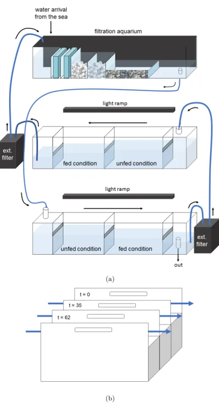
Experiment C: Growth experiment. The growth experiment lasted for two months in a controlled
255
room (temperature, photoperiod) at the Wimereux Marine Station (University of Lille, France)
256
under a recirculating custom seawater system (Fig. 3). In the custom system, one aquarium
257
tray was dedicated to water filtering and two aquaria held the lugworm growing experiment. The
258
seawater, directly pumped from the sea, was kept several days in the filtering aquarium containing
259
fine and coarse filter foam, crushed pozzolana and oyster shells and kept in the dark (Fig. 3).
260
10% of the seawater contained in the two growing aquaria was renewed every day or every second
261
day with the water of the filtering aquarium. Two external filters (Eheim professional 4+ 250)
262
and pumps allowed the circulation and additional filtration of the seawater system (Fig. 3a). A
263
lightening system consisting in two light ramps (Alpheus Radiometrix 13C1001C) mimicking the
264
external light intensity and photoperiod was added to the system (Fig. 3a), air pumps (Air pump
265
8000 and Eheim 400 from Europrix ltd., not represented on Fig. 3) linked to home-made finely
266
punctured pipes allowed the oxygenation of the system. The temperature was kept around 15°C (˘
267
1°C). Each of the two growing aquarium trays were holding each twice 3 boxes filled with sediment
268
burnt at 60°C during 24 h and lugworms (Fig. 3b). The first 3 boxes closer to the seawater arrival
269
were dedicated to the unfed condition, the next 3 to the fed condition. A small waterfall between
270
them prevented the seawater (and food) to circulate in the opposite direction of the main current,
271
thus no food could reach the unfed condition. The design of the boxes and of the separations
272
prohibited the worms to leave their box and to circulate from one condition to another condition
273
(Figs. 3a, b). All lugworms were measured and only individuals ranging from 0.4 cm to 1.6 cm of
274
trunk length were selected. Twelve batches of 30 individuals were made with the same size (trunk
275
length) range. Each batch was placed in a separated box within the experimental set up (Fig. 3b).
276
Feeding occurred twice at t = 0 and t = 35 days with yeast wastes (obtained from Brasserie du
277
pays Flamand ltd., a local brewery) inserted within the sediment with 20 ml syringes (between 1.8
278
and 3.6.1010cells added per box) (Olive et al., 2006). One batch of lugworms of each condition in
279
both aquaria was withdrawn at the beginning of the experiment, after 35 days and after 62 days,
280
kept 24 h in the cold room and weighted and measured.
281
Data analyses. All data analyses were performed on Matlab R2015b. For the oxygen consumption
282
experiment (Exp. A), for each measurement (blanks included), the associated percentage of oxygen
within the tube was calculated according to the Equation (2).
284
O2 measuredp%q “ O2 measuredpV q ´ O2 minpV q
O2 maxpV q ´ O2 minpV q ¨100 (2) With O2 measured(V) the oxygen measured, O2 min(V) the oxygen measured for 0% of oxygen, and
285
O2 max(V) the oxygen measured for 100% of oxygen. The oxygen content (µmol.L-1) was then
286
calculated according to the temperature (T, in °C), salinity (S, in ‰) and the water content of
287
each tube according to Aminot and Kérouel (2004, see on pages 110-118). The blank effect was
288
deleted, and the individual oxygen consumption (µmol.h-1) was then calculated as the inverse of
289
the slope of the linear regression of the evolution of the oxygen content over time. Both conditions
290
were analyzed together to consider an average level of activity.
291
For the reproduction data acquisition, the fecundity (F) was calculated for each female according
292
to Equation (3) (with n the mean of the three counts).
293
F “ n
4 ¨ 10´3 (3)
Since spawning happens only once a year for A. marina, the reproduction rate for each female
294
was calculated as the fecundity divided by the number of days in one year and plotted against the
295
female trunk length (uni-variate data). The wet weight of an egg was calculated as the total weight
296
of oocytes divided by fecundity (zero-variate data).
297
1.2.3. Parameters estimation
298
The parameters estimation of the DEB models was done using the covariation method described
299
by Lika et al. (2011), using the dataset shown in Table 3. The estimation was completed using the
300
package DEBtool (as described in Marques et al., 2018) on the software Matlab R2015b using both
301
a std-DEB model and an abj-DEB model, in order to select the best fit model and to compare the
302
parameter obtained with both models.
303
The parameter estimation procedures were evaluated by computing the Mean Relative Errors
304
(MRE), varying from 0, when predictions match data exactly, to infinity when they do not, and
305
the Symmetric Mean Square Errors (SMSE), varying from 0, when predictions match data exactly,
306
to 1 when they do not (http://www.debtheory.org).
307
1.3. Inferring environmental conditions from biological data and vice versa
308
1.3.1. Functional scaled response associated to growth data
309
The parameters of abj-model for Arenicola marina (best fit model), as well as two different
310
growth datasets, were used to validate the model and infer the environmental conditions (in terms
311
of food levels) of these datasets. The first growth dataset was taken from Beukema and De Vlas
312
(1979). It represents seasonal changes in mean individual dry weight (9-year averages) in small
313
lugworms from two populations of the Wadden Sea. The second dataset consists of the observations
314
of wet weight and trunk length of the experiment C. Since the results of the latest experiment
315
seemed to indicate that food was lacking from t = 35 days to t = 62 days and since no significant
difference between the two feeding conditions were observed, the abj-model applied in this study
317
was used to reconstruct the scaled functional response (f) as a proxy of food levels during the
318
whole experiment for the two conditions. Predictions on these different growth experiments were
319
made at one temperature but for feeding conditions varying from f = 0.02 to f = 1. The best
320
fit predictions were chosen as the ones presenting the smallest sum of squares of the differences
321
between observations and predictions.
322
1.3.2. Life cycle chronology under in situ environmental conditions
323
The abj-DEB model for Arenicola marina was used to reconstruct the chronology of the early
324
life stages of the species under the in situ environmental conditions of Wimereux (Eastern English
325
Channel, Hauts-de-France), as well as its growth in wet weight and trunk length, and compared
326
them with optimal food and temperature conditions (f = 1 and T = 20 °C).
327
Local environmental conditions. The in situ temperature of the year 2017 were taken from
SOM-328
LIT. As a first approximation, the scaled functional response f was guessed from monitoring of the
329
phytoplankton within the Eastern English Channel (Lefebvre et al., 2011) showing higher
abun-330
dances in spring and autumn, as generally observed in the North Atlantic temperate ocean (Miller
331
and Wheeler, 2012, Fig. 11.7).
332
Chronology of the early life-stages and associated lengths. The parameters of the abj-model
pre-333
viously estimated were used to predict age and length at trochophore larva stage, birth,
meta-334
morphosis and puberty under the non-optimal environmental conditions of Wimereux previously
335
defined.
336
Growth predictions. The evolution of the compartments of reserve, structure and reproduction
337
buffer from the fertilization to the lifespan amand further was calculated according to the equations
338
of Table 1. For each environmental condition, the ages for all the life stages were predicted as
339
previously and a temperature correction was applied when the temperature was different from 20
340
°C. The values of E, V and ER over time were then converted into wet weight and/or physical
341
trunk length with the equations found in Table 1.
342
1.4. Comparison of the DEB parameters of Arenicola marina with other Lophotrochozoan species
343
The parameters found with the abj-DEB model for Arenicola marina were compared with the
344
ones found with the std-model, as well as with the parameters of other molluscs and annelid species.
345
The parameters collected were taken from the Add-my-Pet collection (AmP) (Marques et al., 2018)
346
using the function prtStat of the AmPtool package used on Matlab R2015b. All values were given
347
for a reference temperature Tref of 20 °C. The most complete data set for molluscs is for the
348
gastropod Lymnaea stagnalis (completeness = 5). The maximum completeness value for annelids
349
in AmP is 2.8, and is found in two species of polychaetes and four species of clitellates. The least
350
complete data set for molluscs is for the symbiotic bivalve Thyasira cf. gouldi (completeness = 1.5)
and the least complete data set for annelids is for the polychaete Capitella teleta (completeness =
352
1.5).
353
Some of the primary parameters of the two models for A. marina were not compared given the
354
lack of data for these parameters (e.g. the searching rate t 9Fmu, the digestion and the reproduction
355
efficiencies κX and κR), as in Kooijman and Lika (2014). The acceleration factor sM of A. marina
356
was calculated as sM “ Lj{Lb, with Lbthe structural length at birth and Ljthe structural length at
357
the end of the metamorphosis, and compared with the one of other species. For the species showing
358
a metabolic acceleration (sM ą1), the infinite length L8was calculated as L8 “ Lm¨ sM, with Lm
359
the maximum structural length (Lm“ κ ¨ tpAmu
rpMs ). The energy conductance after metamorphosis
360
vj and the maximum assimilation rate after metamorphosis tpAmuj were calculated as vj “ vb¨ sM
361
and tpAmuj “ tpAmub¨ sM, with vb the energy conductance at birth and tpAmub the maximum
362
assimilation rate at birth (Kooijman, 2014; Kooijman and Lika, 2014). All ten parameters, as well
363
as the expectations based on the general animal (Kooijman, 2010, Table 8.1), were represented as
364
functions of L8 for all the considered species.
365
2. Results 366
2.1. Parameter estimation
367
2.1.1. Parameters of the model
368
The completeness of the models was set at 4.2 following Lika et al. (2011) according to the
369
dataset used in the parameters estimation (Table 3). The implementation of the parameter
es-370
timation of the std-DEB model provided a Mean Relative Error (MRE) of 0.30 and Symmetric
371
Mean Square Error (SMSE) of 0.38 (Marques et al, 2018). The implementation of the parameter
372
estimation of the abj-DEB model provided a MRE of 0.23 and SMSE of 0.29. In addition to the
373
fact that the abj-model provided a better fit to the data set, it appears that the std-model largely
374
underestimates the age and length at birth, ab and Lb (the relative errors, RE, are respectively
375
0.91 and 0.83), as well as the age when then trochophore larva appears, atr, (RE = 0.60). For both
376
models, the values of the fraction of the metabolized energy allocated to soma, κ, appeared equal
377
(Table 4). The specific somatic maintenance rate, [ 9pM], and the maximum assimilation rate at
378
birth, t 9pAmub, and at metamorphosis, t 9pAmuj, were respectively five, twenty and two times higher
379
with the std-model than with the abj-model. However, the maturation thresholds for the occurring
380
of the trochophore larva, Etr
H, for birth, EHb , and for puberty, E p
H, and the energy conductance at
381
metamorphosis, 9vj, appeared higher with the abj-model, that considered a metabolic acceleration
382
rate between birth and metamorphosis, sM, around 11 (Table 4).
383
2.1.2. Observations vs predictions
384
Zero-variate data. For 9 of the 12 zero-variate observations of the estimation procedure with the
385
abj-model, the predicted values were close to the observed ones (RE ď 0.27) (Table 5). The last
386
three predictions for the age at birth ab, the age at puberty ap and the total length at birth Lb
showed higher relative errors (RE „ 0.65). The predictions obtained with the std-model estimation
388
procedure were overall less well adjusted to the zero-variate observations with 50% of the predictions
389
associated RE higher than 0.45 (Table 5). For instance, the age at birth ab, the age when the
390
trochophore larva is first observed atr and the age at puberty apwhere highly underestimated with
391
the std-model estimation procedure (RE respectively of 0.91, 0.6 and 0.74), as well as the total
392
length at birth Lband the length when the trochophore larva is first observed Ltr (RE respectively
393
of 0.83 and 0.45).
394
Uni-variate data. The RE of the uni-variate data set ranged from 0.06 to 0.41 with the
abj-395
DEB model, and from 0.08 to 0.42 with the std-DEB model, with, in both cases, the highest
396
values corresponding to the fit to the length-weight data collected on individuals of highly variable
397
reserve and reproduction buffer levels, and to the oxygen consumption data set (most scattered
398
values) (Figs. 4, 5, 6, 7). In both cases, the oxygen consumption increased with the increase of
399
temperature (Fig. 4). The values of the shape coefficients δM varied for a priori the same measure
400
of the trunk length between 0.14 and 0.20 with the abj-DEB model and between 0.09 and 0.13 with
401
the std-DEB model according to the authors (Fig. 7), which is due to the lack of rigid measurable
402
parts in Arenicola marina that could be used as a proxy for length.
403
2.2. Reconstruction of environmental conditions with the abj-model for Arenicola marina from
bi-404
ological data and vice versa
405
2.2.1. Scaled functional response
406
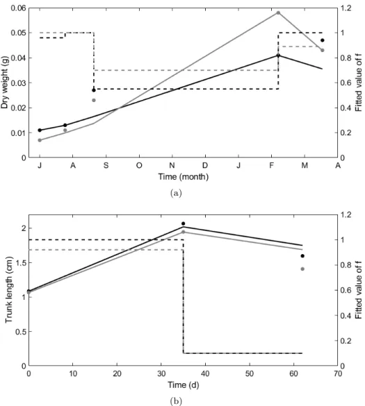
From a field growth dataset. The abj-model provided a good fit for the field growth data taken
407
from Beukema and De Vlas (1979) for the two studied sites (Fig. 8a). The values of the scaled
408
functional response f were shown to evolve on both sites during the year, with the highest values
409
during spring and late summer periods compared to winter period (Fig. 8a).
410
From laboratory growth data. Overall, the abj-model provided a good fit for the growth data
411
obtained in the laboratory (Exp. C), although growth was slightly underestimated between t = 0
412
and t = 35 d, and slightly overestimated between t = 35 and t = 62 d (Fig. 8b). The reconstruction
413
of the scaled functional response f provided indications on the fact that the food levels within the
414
sediment between t = 35 d and t = 62 d might have been really low and did not allow an optimal
415
growth.
416
2.2.2. Chronology and growth during the life cycle according to the environmental conditions
417
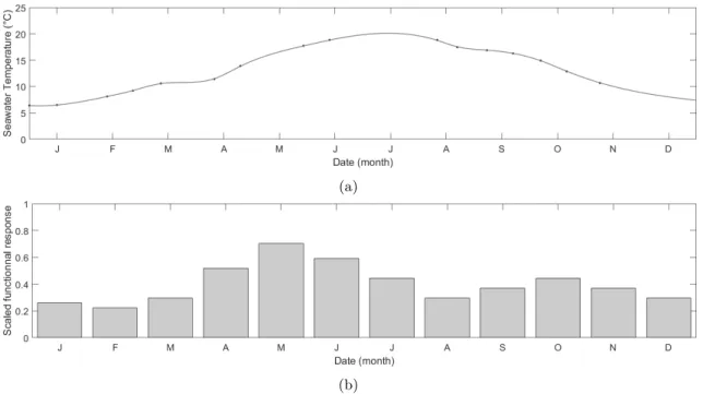
In situ environmental conditions. The seawater temperatures ranged from 5.5 to 20 °C at Wimereux,
418
with the highest temperature between July and September and the lowest temperature between
419
January and February (Fig.9a). The scaled functional response was supposed to range from 0.3 to
420
0.95 with higher values in spring and autumn and lower values in summer and winter (Fig.9b).
Chronology of the first life stages. The abj-model predicted an age at trochophore larva stage atr
422
of 10.3 days and an age at birth ab (used as an approximation of the age at the first settlement)
423
of 15.5 days at Wimereux, considering the environmental conditions presented in Fig. 9 (Table
424
6), suggesting a first dispersal phase in between these two events of around 5 days. The age at
425
the end of metamorphosis aj was predicted to be 208 days (a little less than 7 month) in local
426
environmental conditions, which means around mid April for a spawning period in mid September.
427
The age and trunk length at puberty of the lugworms of Wimereux, ap and T Lp, were predicted
428
to be respectively 373.2 days and 3.5 cm.
429
Wet weight and trunk length growth predictions according to the environmental conditions. The
430
total wet weight of Arenicola marina (considering the structure, reserve and reproduction buffer
431
compartments) predicted by the model at the maximum age amwas around 20 times superior in
432
optimal conditions (f = 1 and T = 20°C, around 400 g) compared to in situ conditions recorded
433
at Wimereux (f = 0.4 and T = 13°C, around 20 g) (Fig. 10). The total trunk length of A. marina
434
predicted by the model was more than twice superior in optimal conditions (f = 1 and T = 20°C,
435
around 33 cm) than in the environmental conditions recorded at Wimereux (f = 0.4 and T = 13°C,
436
around 14 cm) (Fig.11).
437
2.3. Comparison of the abj-DEB parameters of Arenicola marina with other Lophotrochozoan species
438
In annelids and molluscs, the maximum assimilation rate, t 9pAmu, increased with the
maxi-439
mum structural length as expected, and more markedly after metamorphosis and the associated
440
metabolic acceleration phase (Fig. 12). The values for Arenicola marina with the abj-model
ap-441
peared lower than those of most of the other polychaetes and clitellates species before and after
442
metamorphosis, except for the values of Urechis caupo (echiurian species), the only other annelid
443
species for which an abj-model was applied.
444
The value of the maximum assimilation rate after metamorphosis, t 9pAmuj, of A. marina with
445
both models was close to the one expected for the generalized animal, and followed the tendency
446
found in most of the others mollusc species, which was not the case for the other polychaetes species,
447
mostly showing higher values. The allocation fraction to soma, κ, was higher for A. marina („
448
0.92) than the one expected for the generalized animal (0.8), and did not appear inconsistent with
449
the values of κ calculated in molluscs species (Fig. 12). The energy conductance value, 9v, for A.
450
marinaappeared lower in the abj- than in the std-model before metamorphosis, but the opposite
451
happened after metamorphosis, where the abj-model’s value was higher than the generalized animal
452
but closer to molluscs’ values. The specific somatic maintenance costs values, [ 9pM], of A. marina
453
were much lower than those predicted for most of the other species of annelids (except for Urechis
454
caupo) but were close to the one of the generalized animal and are consistent with the values for
455
the molluscs species (Fig. 12). The value of the costs of structure, rEGs, of A. marina appeared
456
equal to those of the other annelids’ and most of the molluscs’ species (Fig. 12). The value of the
maturity maintenance rate coefficient, 9kj, of A. marina was equal to those of the other annelids’
458
and of most of the molluscs’ species (Fig. 12). The values of the maturity thresholds for birth,
459
metamorphosis and puberty, Eb H, E
j
H, and E p
H, of the abj-model for A. marina were lower than
460
those of the generalized animal but similar to most of the mollusc species’ values (Fig. 12).
461
3. Discussion 462
In the present study, we successfully estimated the parameters of both a std- and an abj-DEB
463
model for the lugworm Arenicola marina, combining the use of literature, experimental and field
464
data. We found that the abj-model was more appropriate for modelling A. marina’s energy budget
465
and life cycle and implemented it under field conditions to reconstruct feeding levels as well as A.
466
marina’s growth and life cycle chronology.
467
3.1. Physiological implications of the std- and the abj- parameter estimation results
468
Major differences in the organisms physiology were implied by the parameter results obtained
469
with a faster metabolism for Arenicola marina with a std-DEB model compared to an abj-DEB
470
model. Indeed, t 9pAmub, t 9pAmuj, [ 9pM] and 9vb appeared higher with the std- parameter estimation,
471
and 9vj higher with the abj- parameter estimation. First, a higher value of the maximum
assim-472
ilation rate t 9pAmuimplies a higher value of the assimilation flux from the same amount of food,
473
and a higher value of the energy conductance 9v implies a larger mobilization flux (Agüera et al.,
474
2015). The reserve capacity [Em], defined by the ratio [Em]“ t 9pAmu{ 9v (Montalto et al., 2014) was
475
found to be 16766 J.cm-3 with the std- parameter estimation compared to 1177 J.cm-3 with the
476
abj- parameter estimation (considering a temperature of 20°C). In comparison, [Em] values for
ac-477
celerating molluscs species were estimated around 4500 J.cm-3and [E
m] values for non-accelerating
478
molluscs species were estimated around 11600 J.cm-3(Add-my-Pet collection consulted in
Novem-479
ber 2018). Second, a higher value of the volume-specific maintenance costs, [ 9pM], implies a higher
480
level of energy needed for the same amount of structure acquired. The comparison of the
parame-481
ter estimation of the abj- and std- models therefore resulted on the one hand, with the parameter
482
estimation of the std-model, in one organism able to store more energy in the reserve
compart-483
ment, but also using more energy for the maintenance of its structure, and on the other hand,
484
with the parameter estimation of the abj-model, in one organism able to store less energy in the
485
reserve compartment, but using less energy for the maintenance of its structure. Indeed, although
486
the predictions of the std- and abj- versions of the model were quite similar (except for the early
487
life-stages predictions), they implied really different bioenergetics in two kinds of organisms storing
488
and using energy differently.
489
3.2. Implications of using an abj-model for Arenicola marina in relation with its biology and ecology
490
For Arenicola marina, the abj-model gave better fit results than the std-model (smaller MRE
491
and SMSE), even when only few observations within the data set accounted for the acceleration
period (only the zero-variate observations aj and Lj were added, but no uni-variate observations
493
made between birth and metamorphosis). The presence of a metabolic acceleration between birth
494
and metamorphosis in A. marina might be related to its bentho-pelagic life cycle. Indeed,
acceler-495
ating species have longer incubation time (before birth) than non-accelerating species (Kooijman,
496
2014; Kooijman et al., 2011), which might be linked to the presence of a larval dispersal phase, since
497
a lower metabolism (in comparison with a non-accelerating species, or with juvenile or adult from
498
the same species) allows for more dispersal time, especially when dispersal rate mainly depends
499
on passive water transport (Kooijman, 2014). This seems in accordance with the presence of a
500
dispersal phase happening before birth for A. marina and with the fact that predictions of atrand
501
abof the std- model presented in this study appeared much smaller than observations, compared to
502
predictions made by the abj-model. In lugworms, the gradual change of feeding behaviour between
503
the first feeding at birth, the temporary settlement between birth and metamorphosis, and the
504
semi-permanent settlement after metamorphosis on the foreshores inhabited by adults (Farke and
505
Berghuis, 1979a, b) might be a mechanism of the increase of the metabolic acceleration sM, also
506
increasing the resulting specific assimilation rate (since t 9pAmuj “ sM ¨ t 9pAmub) of the individual.
507
The increase of the organic matter concentration within the water column during spring (spring
508
blooms), before the second dispersal phase when metamorphosis is almost completed, might also
509
play a role in the increase of the specific assimilation rate, increasing the amount of food available
510
for the same feeding effort.
511
3.3. Phylogenetic implications of the use of abj-DEB models for polychaetes
512
The metabolic acceleration rate value for A. marina („ 11) falls in the range of what can be
513
found in mollusc species (for more than 95% of the mollusc species, 1 ď sM ď 27 in the AmP
514
database), which seems consistent with the fact that polychaetes and molluscs both belong to the
515
Lophotrochozoan clade, having both a common trochophore larval stage after the embryogenesis.
516
However, although all annelids are part of the Lophotrochozoan clade, they do not all share the
517
presence of at least one larval dispersal phase during their life cycle, and therefore, might not
518
all experience a metabolic acceleration during their life cycle. As an example, clitellates have a
519
direct development with no larval phase (related to their terrestrial habitat) and std-models might
520
show better fit for these species that may not experience a metabolic acceleration during their life
521
cycle. From an evolutionary point of view, metabolic acceleration might first have been common
522
to all Lophotrochozoans and secondarily lost in clitellate species (as suggested by Marques et al.,
523
2018, for other taxa). Nevertheless, since some species with no larval phase might also experience
524
a metabolic acceleration (Kooijman, 2014), and since metabolic acceleration seem common to a
525
large part of the species belonging to the Lophotrochozoan clade (Kooijman, 2014; Marques et
526
al., 2018), a comparison of the use of both abj- and std- models for clitellate species should be
527
considered.
3.4. Energy budget and in situ life cycle predictions
529
The predictions on the chronology of Arenicola marina’s life cycle stages under the in situ
530
environmental conditions met at Wimereux (metamorphosis completed at around 7 months, in
531
mid April) seemed in accordance with observations made by De Cubber et al. (2018), who spotted
532
the first recruits of the species (e.g. juveniles after metamorphosis) in May at the same site.
533
This would suggest a second dispersal period of less than one month if lugworms migrate after
534
metamorphosis. Moreover, the age and length at puberty of the lugworms at the Wimereux site
535
were predicted with the abj-model to be respectively 373.2 days and 3.5 cm, which is close to the
536
observations made by De Cubber et al. (2018) with a length at first spawning (after the acquisition
537
of maturity) of 3.8 cm and an age of 1.5 to 2.5 years. Newell (1949, 1948) reported the presence
538
of A. marina metatrochophore larvae close to birth (and thus close to the first settlement stage)
539
with 3 to 4 setigers and around 0.034 cm of length around 2 to 3 weeks after the occurrence of the
540
spawning event at Whistable (UK) (limit between the English Channel and the North Sea). His
541
observations also seem in accordance with the abj-model predictions. Indeed, the age and length at
542
birth predictions at Wimereux in October were of 15.5 days and 0.034 cm. Since temperatures are
543
lower in November in the English Channel and even lower in the North Sea, birth might have been
544
slightly delayed in their study and their observations seem to be in accordance with the abj-model
545
implemented in our study. Observations of post-larvae in mucus tubes were commonly made on
546
fucus and pebbles areas until the end of February (Benham, 1893; Newell, 1949, 1948) and up to
547
April in some cases (Newell, 1949). First settlements of juveniles on adult grounds were reported
548
by Newell (1949, 1948) at the end of April or beginning of May, which is in accordance with our
549
model predictions (after the age at metamorphosis, which is around 5 months-old) and correspond
550
to a dispersal period after metamorphosis of a maximum of one month.
551
The biggest individuals of A. marina collected at the studied sites might give indications on the
552
in situ environmental conditions met by the lugworms on these sites. Indeed, at Wimereux, the
553
heaviest individual collected by the authors between 2015 and 2018 weighted 10 g and the longest
554
one measured 15.2 cm of trunk length (data not shown), which is in accordance with the length and
555
weight predicted by the abj-model for Arenicola marina at an age of 5 to 6 years old (age of the last
556
cohort calulated by De Cubber et al. (2018)) for f = 0.4 and T = 13°C. At Le Touquet (Eastern
557
English Channel, De Cubber et al., 2018), the heaviest individual collected weighted 53.1 g and
558
the longest one measured 20.2 cm of trunk length (data no shown), and at Fort Mahon (Eastern
559
English Channel, De Cubber et al., 2018), the heaviest individual collected weighted 26 g and the
560
longest one measured 18.4 cm of trunk length (data not shown). Since no major difference between
561
the seawater temperature at the three different sites exist, the main difference was possibly the food
562
availability. The comparison of these biometric values with the ones predicted by the abj-model
563
(around 600 g of maximum wet weight and 35 cm of maximum trunk length for f = 1 and T =
564
13°C) seems to indicate that f was higher at Le Touquet and Fort Mahon compared to Wimereux.
In the different sites of the Eastern English Channel cited previously, De Cubber et al. (2018)
566
showed that the lugworms’ recreational harvest in 2017 removed more than 500 000 lugworms and
567
represented a total retail value of around 232 447 euros. The need for implementing management
568
measures was also evidenced for at least one beach by these authors. Knowing the food levels of the
569
different sites might then enable predictions with the abj-model on the in situ ages and lengths at
570
puberty, which could help managers to implement relevant regulations if needed such as a relevant
571
harvest minimum size limit on the different sites showing highly variable food levels and maximum
572
lengths and weights.
573
3.5. Possible future extensions of the model
574
In order to provide the best model possible for Arenicola marina further adjustments could be
575
implemented linked to the species life cycle and habitats. First, defining the temperature tolerance
576
range of the species could improve the abj-model by applying better temperature corrections.
577
Growth experiments from Farke and Berghuis (1979) seem to point out a higher boundary of
578
the temperature tolerance range TH around 25 °C. Other studies suggest a lower boundary of
579
the temperature tolerance range TL under 5°C (Sommer et al., 1997; Wittmann et al., 2008),
580
but no Arrhenius temperatures beyond the temperature tolerance (TAH and TAL) range could
581
be calculated yet. Further experiments on growth or respiration under temperatures beyond the
582
temperature tolerance range could be performed to define TAH and TAL and thus improve the
583
temperature correction.
584
During their life cycle, the different stages of A. marina inhabit different marine habitats with
585
different ranges of temperature variation. From the metatrochophore to the post-larval stage the
586
lugworms inhabit the subtidal area were seawater temperature does not fluctuate that much daily,
587
compared to the intertidal areas inhabited by the juveniles and adults, where temperature can
588
change dramatically during one day. As an example, a variation of 15°C was recorded within
589
the sediment at the Wimereux site in November 2017 (Fig. 13). In this study, the Arrhenius
590
temperature was calculated from the oxygen consumption rate of juveniles living on the upper
591
shore. We hypothetize that a different Arrhenius temperature may exist for the larval and
post-592
larval stages living in habitats with a more stable temperature, as suggested by Kooijman (2010).
593
Further experiments could be implemented on larvae in order to record physiological rates and
594
estimate their Arrhenius temperature.
595
Monaco and McQuaid (2018) highlighted the interest of adding to the temperature correction
596
an aerial exposure term Md (linked to tidal height and the position of organisms on the shore) in
597
foreshore habitats showing wide fluctuations in temperature and desiccation. Given the intense
598
variations experienced by juvenile and adult lugworms (Fig. 13), it might be interesting to add an
599
aerial exposure term for the species. Indeed, the underestimation of growth by the model compared
600
to our observation of growth of juveniles in the laboratory (Exp. C) might be linked to the fact
601
that no tide was simulated and lugworms stayed immersed during all the experiment time, without
the stress brought by high temperature variations and aerial exposure. However, it was found that
603
lugworms gradually migrate down the shore while growing (De Cubber et al., 2018), so the aerial
604
exposure correction, if implemented, should gradually decrease during the life cycle of the organism
605
as well.
606
DEB models as implemented here enable to reconstruct the growth and the reproduction of
607
a species at the individual level. However, in order to be used in a population context, DEB
608
theory can be associated to individual-based models (IBM) in order to explore properties of both
609
individual life-history traits and population dynamics (Bacher and Gangnery, 2006; Martin et al.,
610
2012). The association of the abj-model developed here, and providing predictions on the duration
611
of the larval dispersal phase, with biophysical larval dispersal models (Nicolle et al., 2017) could
612
also allow the understanding of the populations’ connectivity in the area and thus give valuable
613
information for the conservation of the species.
614
Acknowledgements 615
We would like to thank D. Menu for his help in the design and creation of the growth system, and
616
V. Cornille for his technical support on the field. This work was partly funded by the University of
617
Lille and CNRS. We are grateful to Europe (FEDER), the state and the Region-Hauts-de-France for
618
funding the experimental set up and T. Lancelot (research assistant) through the CPER MARCO
619
2015 - 2020. L. De Cubber is funded by a PhD studentship from the University of Lille. Finally
620
we would like to thank Starrlight Augustine and an anonymous reviewer for their comments that
621
help improving this manuscript.
622
References 623
Agüera, A., Collard, M., Jossart, Q., Moreau, C., Danis, B., 2015. Parameter
estima-624
tions of Dynamic Energy Budget (DEB) model over the life history of a key antarctic
625
species: The antarctic sea star Odontaster validus (Koehler, 1906). PLoS One 10, 1–23.
626
https://doi.org/10.1371/journal.pone.0140078
627
Aminot, A., Kerouel, R., 2004. Hydrologie des écosystèmes marins; paramètres et analyses,
628
Ifremer. ed.
629
Bacher, C., Gangnery, A., 2006. Use of dynamic energy budget and individual based models
630
to simulate the dynamics of cultivated oyster populations. J. Sea Res. 56, 140–155.
631
Benham, W.B., 1893. The Post-Larval Stage of Arenicola marina . J. Mar. Biol. Assoc.
632
United Kingdom 3, 48–53. https://doi.org/10.1017/S0025315400049559
633
Beukema, J.J., De Vlas, J., 1979. Population parameters of the lugworm Arenicola
ma-634
rinaliving on tidal flats in the Dutch Wadden Sea. Netherlands J. Sea Res. 13, 331–353.
635
Blake, R.W., 1979. Exploitation of a natural population of Arenicola marina (L.) from the
637
North-East Coast of England. J. Appl. Ecol. 16, 663–670. https://doi.org/10.2307/2402843
638
Cadman, P., Nelson-Smith, A., 1990. Genetic evidence for two species of lugworm (Arenicola)
639
in South Wales. Mar. Ecol. Prog. Ser. 64, 107–112. https://doi.org/10.3354/meps064107
640
Cadman, P.S., Nelson-Smith, A., 1993. A new species of lugworm: Arenicola defodiens sp.
641
nov. Mar. Biol. Ass. U.K 73, 213–223. https://doi.org/10.1017/S0025315400032744
642
De Cubber, L., Lefebvre, S., Fisseau, C., Cornille, V., Gaudron, S.M., 2018. Linking
life-643
history traits, spatial distribution and abundance of two species of lugworms to bait
col-644
lection: A case study for sustainable management plan. Mar. Environ. Res. https://
645
doi.org/10.1016/j.marenvres.2018.07.009
646
De Wilde, P.A.W.J., Berghuis, E.M., 1979. Laboratory experiments on growth of juvenile
647
lugworms, Arenicola marina. Netherlands J. Sea Res. 13, 487–502. https://doi.org/10.1016/
648
0077-7579(79)90020-6
649
Farke, H., Berghuis, E.M., 1979a. Spawning, larval development and migration of Arenicola
650
marinaunder field conditions in the western Wadden sea. Netherlands J. Sea Res. 13,
651
529–535.
652
Farke, H., Berghuis, E.M., 1979b. Spawning, larval development and migration behaviour of
653
Arenicola marinain the laboratory. Netherlands J. Sea Res. 13, 512–528.
654
Galasso, H.L., Richard, M., Lefebvre, S., Aliaume, C., Callier, M.D., 2018. Body size and
655
temperature effects on standard metabolic rate for determining metabolic scope for activity of
656
the polychaete Hediste (Nereis) diversicolor. PeerJ 1–21. https://doi.org/10.7717/peerj.5675
657
Kooijman, S.A.L.M., 2014. Metabolic acceleration in animal ontogeny: An evolutionary
658
perspective. J. Sea Res. 94, 128–137. https://doi.org/10.1016/j.seares.2014.06.005
659
Kooijman, S.A.L.M., 2010. Dynamic energy budget theory for metabolic organisation.
Cam-660
bridge University Press.
661
Kooijman, S.A.L.M., Lika, K., 2014. Comparative energetics of the 5 fish classes on the basis
662
of dynamic energy budgets. J. Sea Res. 94, 19–28. https://doi.org/10.1016/j.seares.2014.01.
663
015
664
Kooijman, S.A.L.M., Pecquerie, L., Augustine, S., Jusup, M., 2011. Scenarios for
accel-665
eration in fish development and the role of metamorphosis. J. Sea Res. 66, 419–423.
666
https://doi.org/10.1016/j.seares.2011.04.016