Design procedures for equiripple nonrecursive digital filters.

¢-

~

ROOM& 36-

i

OCUmT OFFICE ,W

i

RESEARCH

il

S.

MASSACHUSETTS INSITUTE, OF ...

A

DESIGN PROCEDURE FOR EQUIRIPPLE

NONRECURSIVE DIGITAL FILTERS

OR.

' :

RICHARD W. HANKINS

LOAN

COPY

TECHNICAL REPORT 485

MASSACHUSETTS INSTITUTE OF TECHNOLOGY

RESEARCH LABORATORY OF ELECTRONICS

CAMBRIDGE, MASSACHUSETTS 02139

The Research Laboratory of Electronics is an interdepartmental laboratory in which faculty members and graduate students from numerous academic departments conduct research.

The research reported in this document was made possible in part by support extended the Massachusetts Institute of Tech-nology, Research Laboratory of Electronics, by the JOINT SER-VICES ELECTRONICS PROGRAMS (U. S. Army, U. S. Navy, and U. S. Air Force) under Contract No. DAAB07-71-C-0300.

Requestors having DOD contracts or grants should apply for copies of technical reports to the Defense Documentation Center, Cameron Station, Alexandria, Virginia 22314; all others should apply to the Clearinghouse for Federal Scientific and Technical Information, Sills Building, 5285 Port Royal Road, Springfield, Virginia 22151.

THIS DOCUMENT HAS BEEN APPROVED FOR PUBLIC RELEASE AND SALE; ITS DISTRIBUTION IS UNLIMITED.

MASSACHUSETTS

INSTITUTE OF TECHNOLOGY

RESEARCH LABORATORY OF ELECTRONICS

Technical Report 485

May 12, 1972

DESIGN PROCEDURES FOR EQUIRIPPLE

NONRECURSIVE DIGITAL FILTERS

Richard W. Hankins

Submitted to the Department of Electrical

Engineering at the Massachusetts Institute

of Technology, November 19, 1971, in

par-tial fulfillment of the requirements for the

degree of Master of Science.

(Revised manuscript received January 12, 1972)

(Revised Appendices received May 5, 1972)

THIS DOCUMENT HAS BEEN APPROVED FOR PUBLIC

RELEASE AND SALE; ITS DISTRIBUTION IS UNLIMITED.

Abstract

A design procedure for the class of nonrecursive digital filters exhibiting

equi-ripple passband and stopband characteristics is presented. With this method it is

pos-sible for a designer to obtain the coefficients necessary to realize a desired filter without having to implement the design algorithm on a general-purpose digital

com-puter. This method also enables the designer to examine several alternative designs

before deciding on a particular solution. In particular, using a recently proposed

algorithm, we have generated designs for more than 500 filters and systematically catalogued them in both tabular and graphical form. Design curves relating the various filter parameters are presented, as are relations for estimating the required filter

specifications and for interpolation on the curves between tabulated designs.

Trans-formations are included to cover highpass filter design and to enable the design of other sets of filters not explicitly catalogued. Sections are included to demonstrate the

use of the design curves and tables and to discuss nonlinear phase filters. An

appen-dix by Joseph Siegel gives the computer program used to generate the design solutions.

TABLE OF CONTENTS

I. INTRODUCTION

II. EQUIRIPPLE APPROXIMATION TO IDEAL LOWPASS DESIGN

III. LAGRANGE INTERPOLATION DESIGN ALGORITHM

IV. FILTER SPECIFICATION AND RANGE OF PARAMETERS

V. LAYOUT OF DESIGN TABLES AND DESIGN CURVES

VI. FORMULAS FOR ESTIMATING DESIGN PARAMETERS

VII. USE OF DESIGN CURVES AND TABLES

7. 1 Lowpass-Filter Design

7.2 Design of Filters Derivable from Listings 7.3 Highpass-Filter Design

7.4 Nonlinear-Phase Filter Design 7.5 Interpolation on the Design Curves

VIII. CONCLUSION

Appendix A Design Tables

Appendix B Design Curves

Appendix C Unit Sample Response Listing

Appendix D Design Program

Acknowledgment References iii 1

5

8

16

I. INTRODUCTION

Nonrecursive digital filters have traditionally enjoyed advantages not obtainable by

recursive realizations. These filters can be designed to approximate a given magnitude

frequency response to a desired accuracy and also to have an exactly linear phase. This

last property follows directly from the fact that nonrecursive digital filters have a unit

sample response of finite duration.

Consequently, a zero-phase filter can first be

designed by prescribing the unit sample response to be a real and even function.

Then

by cascading this filter with a finite delay equal to the negative time portion of the filter

unit sample response, a realizable system can be obtained. Since the effect of this finite

delay is to introduce a linear phase term into the frequency response, the resulting

sys-tem is a realizable, nonrecursive digital filter exhibiting an exactly linear phase

charac-teristic. Additionally, since the transfer function of a nonrecursive digital filter has no

poles in the finite z plane, instability resulting from coefficient inaccuracy is not a

problem, as it is in recursive filter design.

Until recently, nonrecursive digital filters were most commonly realized by direct

convolution, a process which becomes increasingly impractical as the filter order is

allowed to increase.

This disadvantage no longer holds when we apply the Fast Fourier

Transform (FFT) algorithm to implementation of high-order filters and adapt

power-ful optimization techniques to the approximation problem. Now it is practical to design

filters of arbitrary order.

The net result of these developments has been a renewed

interest in the design of frequency selective, nonrecursive digital filters.

The approximation problem in the design of nonrecursive digital filters basically

involves obtaining a suitable approximation to a generally specified or ideal frequency

response. As distinguished from the recursive case, in which the realizable

approxi-mations can be expressed as a ratio of two trigonometric polynomials and the extensive

results of analog filter theory can be applied via the bilinear transformation, the

realiz-able nonrecursive approximations are constrained to be trigonometric polynomials and

the bilinear transformation is not applicable. At present, there are several methods

for approximating a desired frequency response with a nonrecursive digital filter. A

few of these methods will be briefly discussed.

1. 1 WINDOWING

Perhaps the most widely used technique for approximating a specified frequency

characteristic has been to approximate the infinite duration unit sample response of

an ideal filter with the finite-duration unit sample response of a nonrecursive

realiza-tion. Since direct truncation of the ideal filter unit sample response results in the

Gibbs phenomenon, a fixed percentage overshoot and ripple in the vicinity of a

discontinuity, it is necessary in practice to modify this unit sample response by

mul-tiplication with a time-limited window or weighting function.

The effect of this

multi-plication in the time domain is a complex convolution in the frequency domain which

1

smooths the spectrum of the filter. Appropriate choice of the window function leads to frequency characteristics with appreciably less in-band and out-of-band ripple, and

acceptable filter designs. The criterion requiring the weighting function to have a trans

-form with a narrow main lobe of high-energy content and small sidelobes with signifi-cantly less energy content has resulted in many useful designs which have been

sum-marized by Rabiner,l Kaiser, and Helms.

1.2 FREQUENCY SAMPLING

Rabiner, Gold, and McGonegal have developed another technique, originally

pro-posed by Gold and Jordan, for the design of nonrecursive digital filters. This method

involves an initial specification of the desired frequency response at a certain number of

uniformly spaced frequency samples. The number of these samples is taken to be the

duration of the filter unit sample response, and the frequency samples are designated

as the discrete Fourier transform of this unit sample response. As a result, the

con-tinuous frequency response is linearly related to the specified frequency samples and is exactly determined as an interpolation between them.

Sampling of the frequency response of an ideal filter generally results in aliasing of the unit sample response and in overshoot and rippling of the frequency

characteris-tics between sample points. In order to improve the frequency response at intersample

frequencies, a number of frequency samples at the band edges are varied in magnitude

so as to increase the transition bandwidth and reduce the ripple variations. Then,

using a linear search and optimization algorithm, the values of these transition-band frequency samples are varied to minimize the maximum deviation between the desired

and designed filter characteristics over some prescribed frequency range. Increasing

the number of samples in the transition band provides for even better ripple cancellation. Practical considerations, however, limit the number of unconstrained variables that can be varied simultaneously, and hence limit the degree to which the ripple can be sup-pressed.

1.3 NONLINEAR OPTIMIZATION

Herrmann and Schuessler ' have developed a third technique for the design of

non-recursive digital filters. This technique can be used to design filters with

equi-ripple passband and stopband characteristics. The maximum allowable ripple values

for both the passband and stopband are prescribed independently, as are the number of

passband ripples Np, and the number of stopband ripples Ns. With N = N + N - 1, a

set of 2N nonlinear equations are then prescribed to constrain the frequency characteris-tic of the filter to the desired tolerance scheme. These equations force an Nthorder poly-nomial to have extrema that achieve the maximum allowable ripple values and to have

zero slope at the frequencies where the extrema occur. The equations are then

itera-tively solved by means of a nonlinear optimization technique to yield the N-1 unknown

yields good results for filters of moderate order, but as the number of unknowns becomes large available algorithms fail to converge; the suitability of this method is therefore restricted.

1.4 LAGRANGE INTERPOLATION

The windowing and frequency sampling techniques do not generally yield filters with equiripple characteristics. Hence they are suboptimal in the sense that they do not yield filter characteristics with the smallest possible transition bandwidth for fixed passband and stopband tolerances. It is possible to modify the method presented by Rabiner et al.4 to yield equiripple designs, but more work is necessary before an objective evaluation of the procedure can be made. On the other hand, the approach taken by Herrmann and

Schuessler6, 7 does yield equiripple characteristics, but is restricted to the design of filters of relatively modest order.

A new technique presented by Hofstetter, Oppenheim, and Siegel8'9 appears to avoid

the computational difficulties encountered with the nonlinear optimization technique and

still provides an equiripple design. Following the terminology first adopted by

Herrmann and Schuessler, the design approximation for a lowpass filter is specified in terms of 5p, the maximum allowable deviation in the passband; s,the maximum allowable deviation in the stopband; Np, the maximum number of passband ripples; and Ns, the

maximum number of stopband ripples. Use of the design algorithm results in a filter with the maximum number of passband and stopband ripples and the minimum duration unit

sample response of 2N+l samples, where N = Np +Ns -1, and the ripple specifications

have included extrema located at frequencies of zero and r radians. A more detailed

explanation of the design algorithm is presented in Section III.For now it can be described as an iterative procedure which, through the use of the Lagrange interpolation formula, evolves from an initial estimate of the set of extremum frequencies to the desired con-tinuous frequency response.

It can be shown8 that of all filters satisfying the type of tolerance scheme mentioned above the subset with the narrowest transition bandwidth occurs when the frequency char-acteristics are specified to be equiripple. It can also be shown that there exists a unique set of filter coefficients yielding this equiripple behavior when the frequency response is real. Since the Lagrange interpolation method is optimal, in that it provides for equi-ripple designs, and since it can be used to design filters of arbitrarily large order, it is the method that will be considered throughout the rest of this report.

The Lagrange method, like the other iterative techniques, has one drawback. Because of its iterative nature the design algorithm must be implemented on some type of

general-purpose digital computer. As a result, a filter designer wishing to use any of the

itera-tive or optimization techniques discussed here would first have to program the design

algorithm or adapt an existing algorithm to his particular needs. Then he would still

have to expend a significant amount of computer time to generate one particular solu-tion, and if he needed to compare several alternative designs, he would have to generate

3

individual solutions for each.

It is apparent that such a procedure could become

both costly and time-consuming and that an alternative method is required.

The method proposed here is to provide the filter designer with a

comprehen-sive set of design curves and tables that will facilitate the design and

implemen-tation of the class of equiripple nonrecursive digital filters discussed by Hofstetter

et al.8 Designs are catalogued both in tabular and graphical form for many standard

filters used in practice.

Confronted with the design problem for a generally specified

filter characteristic, the designer may survey the design curves for the solution to his

particular problem.

If the filter in question is one of the many explicitly catalogued,

the designer need only retrieve the filter coefficients from the tabular data. If the

par-ticular filter has not been explicitly catalogued the curves and tables may be used to

compare catalogued designs and make reasonable trade-offs to arrive at a compromise

solution. Finally, if none of the catalogued designs are acceptable, the designer may

use the design curves and the general specifications of his filter to obtain the design

parameters necessary for an exact computer solution of his problem.

The Lagrange interpolation method is applicable to the design of generally specified

frequency characteristics including conventional lowpass, highpass, bandpass, and

band-stop filters, as well as to the design of piecewise-constant and some

nonpiecewise-constant frequency characteristics.

Throughout this report the discussion is generally

phrased in terms of nonrecursive lowpass digital filters with equiripple band

charac-teristics and linear phase. Sections are included, however, to cover transformations

from the lowpass designs to other types of filters such as highpass designs, and to

dis-cuss filters with nonlinear phase characteristics.

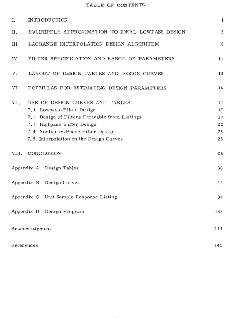
II. EQUIRIPPLE APPROXIMATION TO IDEAL LOWPASS DESIGN

The frequency response of an ideal lowpass filter is unity in the passband and zero

in the stopband.

Because of the sharp step discontinuity and zero transition bandwidth

implied by this characteristic, the ideal filter (shown in Fig. 1)cannot be realized exactly

in practice.

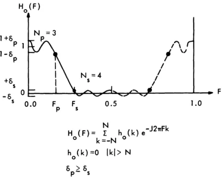
Instead, the equiripple approximation (Fig. 2) which provides for an

allowed deviation about one in the passband and about zero in the stopband as well as for

a nonzero transition band, will be realized via a nonrecursive digital filter with linear

phase. The following notation, illustrated in Fig. 2, is used throughout this report.

Symbol

H(z)

Ho(z)

F

f

T

5

p

6

N

p

N

N= N +N -1

F

p

F

Fk; k= 1, ... , N+1

TBW = IF -Fp

Definition

Transfer function of the linear-phase filter

Transfer function of the zero-phase filter

Normalized frequency = fT

Analog frequency

Sampling interval

Maximum allowable deviation about one in the passband

Maximum allowable deviation about zero in the stopband

Maximum number of passband ripples (including one at F = 0)

.Maximum number of stopband ripples (including one at F= 0.5)

Order of the Lagrange interpolation polynomial

Passband cutoff frequency, at which the frequency

character-istic first leaves the passband

Stopband cutoff frequency, at which the frequency

character-istic enters and remains in the stopband

Extrema frequencies at which ripples achieve their allowed

maximum values

Width of the transition band between passband and stopband

MAGNITUDE

1

0

e

PASSBAND

0.0

0.5

1.0

F=fT

Fig. 1.

Ideal lowpass filter frequency response.

5

Ho (F)

1+6

P- 1

P

+6

s o

-6

tl

CAL

F

=fT

0.0

Fp

FN

0.5

p+l

Fig. 2.

Equiripple approximation to ideal lowpass design.

In these terms linear phase, equiripple, nonrecursive digital filters can be described

by a transfer function of the form

N

(z N+k+z N-k

H(z)

ZN

-

a

kZ

N-k)

(1)

z k=O

Evaluating the complex variable z at z = exp(j2rF) yields the frequency response

N

H(z) z=ejZTF = H(e

= exp(-j2TrFN)

ak cos

(2)

k=O

which can be put in the form

H(e

TF) = exp(-j2rFN) H (F).

(3)

With the filter coefficients constrained to be real, the frequency response is composed

of a linear-phase term exp(-j2rFN) and the purely real frequency response Ho(F) of a

zero-phase filter. Since the linear-phase term only introduces a finite delay of N samples

into the filter unit sample response, the design problem becomes one of fitting Ho(F

,

a mirror-image polynomial, to the tolerance scheme prescribed in Fig. 2. Since Ho(F)

is a real mirror-image polynomial, its zeros must occur in complex conjugate

recip-rocal pairs on or about the unit circle. (This and other properties of mirror-image

which can also be put in the form

N

k

N

Ho(F) = c

Ck(cos

k=O k=O

where x

=

cos

2TF.

As a result, the approximation problem reduces to one of

approxi-mating

a generally prescribed lowpass frequency characteristic with a trigonometric

polynomial.

7

III. LAGRANGE INTERPOLATION DESIGN ALGORITHM

The technique used to achieve this trigonometric polynomial approximation to an

ideal lowpass design was proposed by Hofstetter, Oppenheim, and Siegel.8' 9 Given

desired values for N, Np, 6, and 6s, the design algorithm first estimates an initial set

of extremum frequencies F(0); k = 1, 2, ... , N+1 at which the extrema of the desired

frequency response Ho(F) are to be located. It then uses the barycentric form of the

Lagrange interpolation formula to obtain an N th-order polynomial that passes through the maximum ripple values (1±6p in the passband and ±6s in the stopband) at these

prescribed frequencies. In general, this first Lagrange polynomial will achieve its

extrema at frequencies distinct from the estimated set of original frequencies F(_k0 ) and

additional stages of the algorithm will be required. The second stage of the algorithm

locates the frequencies associated with the extrema of the first Lagrange polynomial and uses these new frequencies F( ) ; k = 1, 2, ... , N+1 as a revised estimate of the

set of extremum frequencies at which the desired frequency response is to achieve

its maximum ripple values. The cycle is completed when a second Lagrange

inter-polation polynomial is constructed so as to pass through the specified ripple values at

this second set of estimated extremum frequencies. At this point the extremum

fre-quencies Fk 2 ) ; k = 1, 2, .. , N+1 of this second Lagrange polynomial can be located,

and if different from the Fk ) the algorithm can proceed iteratively to the desired

solution.

In practice, the iterations were terminated and the algorithm was determined to

have reached a solution when all of the extremum frequencies F); k = 1, 2, ... ,

k k=, -1)

N+1 at the last iteration were equal to the corresponding set of frequencies F k

k = 1, 2, ... , N+1 used in the previous iteration. A formal mathematical proof of

con-vergence is not available, but in our set of reference designs compiled for more than 500 filters covering a wide range of specified tolerances and including filter responses as long as 255 samples, we have found that the algorithm converged quite rapidly to the desired solution in every case.

All of the design solutions tabulated in Appendix A were generated on an IBM 360 computer using a version of the Lagrange interpolation algorithm programmed by Joseph Siegel (Appendix D). Only minor modifications of the program were made to increase its

efficiency in the design of large sets of filters and to insure convergence for a few anomalous cases.

Direct use of the design algorithm yields a set of coefficients and a set of extre-mum frequencies Fk; k = 1, 2, ... , N+1 that completely define the continuous frequency response Ho(F) of the desired filter through the Lagrange interpolation formula. Important as these quantities may be, they are not of much practical use to the

fil-ter designer who wants to implement a particular design. For this reason, the filter

unit sample response h(n); n = -N, -N+1, ... , ...0, , N-i, N is included as part of the specifications for each tabulated design.

The actual filter coefficients, the ak of Eq. 4, are easily related to the filter unit

sample response, as we see by noting that if h (n) represents the unit sample response

of the specified zerg-phase filter, then the frequency response can be written

N

H (F)=

h (k) e

Fk

k=-N

(6)

Note that the summation index ranges only over a set of ZN+l values, since ho(k) is

identically zero for Ik > N.

Equation 6 can be rewritten

N

H (F) = ho(0

+

~k=l

1

-N

h (k) e

1Fk +

Z

h (k) e

ZFk

Since ho(n) was specified to be a real and even function,

Ho(F

=

ho(0

+

h (k)(e

+e

k=l 1

-j 2Fk )

and finally

N

Ho(F)= ho(

+

2h (k) cos ZrTFk.

k=

1

We see that Eqs. 9 and 4 are exactly of the same form, and that the filter coefficients

are related to the filter' s unit sample response by the equations

a

=

h

(0)

and

(10)

ak = Zho(k);

k= 1, Z,...,N.

More generally, it is known that the unit sample response of a nonrecursive digital

filter with duration M samples is related to the M point sequence

H(eTF) I F=n/M;

F2F~E=nM

n = 0, 1, ...

, M-1

formed by sampling the continuous frequency response at a set of M equally spaced

points on the unit circle.

In particular, the inverse discrete Fourier transform

rela-tion reveals that the filter unit sample response can be obtained from the calcularela-tion

h(n) =

H(ej(2

)/M) e

j(2rrkn)/M

M k= 0

n= 0, 1, 2,...,M-1.

This method was modified to take advantage of the symmetries inherent in the filter

9

(7)

(8)

(9)

(11)

I__·I-specifications, and the unit sample response for each of the tabulated filters was

cal-culated in double-precision arithmetic by a subprogram incorporated in the main

design program. Perhaps it would have been more efficient to evaluate the inverse

dis-crete Fourier transform by means of the fast Fourier transform (FFT) algorithm, but for

most of the catalogued filters the saving in computer time would have been insignificant.

The subprogram DFT (discrete Fourier transform) essentially requires N

arithmetic

operations to specify a unit sample response, while the FFT requires approximately

M log

M operations, where M is the next largest power of 2 above 2N+1.

Con-sidering M= 2N and N= 128, we find in this case that the DFT requires approximately

16, 000 operations and the FFT approximately 2000. With each operation performed

in

10

s, use of the FFT would result in a saving of -0. 14 s.

Also, since the most

readily available form of the FFT was implemented only in single-precision

arith-metic, we decided to use the subprogram DFT.

Although all of the designs that are catalogued are of the lowpass variety, the

algo-rithm as programmed is capable of designing bandpass as well as lowpass filters

and, through simple transformations, is also applicable to bandstop and highpass filter

design.

Furthermore, as explained elsewhere,

the Lagrange interpolation method

is amenable to the design of filters with more generally specified frequency

char-acteristics, including lowpass and frequency-selective differentiators, as well as

fil-ters with piecewise-constant characteristics.

IV. FILTER SPECIFICATION AND RANGE OF PARAMETERS

Use of the Lagrange interpolation design algorithm requires the initial specification

of the parameters and 6 , as well as any two of the three parameters N, N p, or N

p s p s

The resulting design has a frequency characteristic with Np passband ripples, each

achieving a maximum value of 1 + 6 p, N stopband ripples of maximum height

±

p s s

certain cutoff frequencies Fp and F s. An important consequence of this specification is that neither the passband cutoff frequency Fp nor the stopband cutoff frequency Fs can be

initially prescribed. As a result with fixed-order (2N+1), fixed 6p, and fixed 6 , there

are only N unique values that Np can assume. Since a unique value of Np implies a unique pair of cutoff frequencies, Fp and F _s, there are, under these constraints, only N different filters available. In order to cover a broader range of possible cutoff frequencies it is

necessary to vary one, or any combination, of the other filter parameters N, 6 , and

6s. The value of the parameter N can range over the set of positive integers, while

the parameters 6 and 6 can assume a continuum of possible values. Hence, although

p s

it is not possible to prescribe the desired cutoff frequencies in advance, in practice any pair of frequencies can be obtained by proper specification of the other filter param-eters. Significantly, the lowpass-lowpass transformation used to obtain any desired cutoff frequency for recursive filters is not applicable here, since it introduces poles into the filter transfer function and distorts the phase characteristic.

In compiling the set of reference designs presented in Appendix A there were two

broad objectives. First, we wanted to cover as wide a range of design specifications

as possible so that many of the standard filters used in practice could be incorporated in the tables and so that the validity of the design algorithm could be tested. Second, we wished to vary the various filter parameters in increments small enough that there would be no large gaps in the data presented. Given a fixed amount of computer time with which to fulfill these objectives, it is apparent that they presented conflicting goals.

Nevertheless, guided by previously tabulated analog filter designs, intuition, and

pre-liminary research data, a choice was made as to the range of values of the design parameters.

The parameter N was allowed to assume the values 5, 7, 10, 15, 31, 63, and 127, corresponding to filter orders of 11, 15, 21, 31, 63, 127, and 255. Note that for the higher order filters the length of the unit sample response (2N+1)was chosen as the next lowest

integer to a power of 2. This choice of values facilitates the implementation of these

filters when realized by the fast Fourier transform or when used as finite

duration-time windows for spectral analysis and estimation. Proportionally fewer high-order

filters were included in the tables because they required significantly more computer

time than low-order solutions. It would be totally inaccurate to conclude from the

selected list of values that the design algorithm failed to converge for the high-order cases. In fact, it converged quite rapidly, within 7 iterations, for filters of order 255, and there is no indication that it cannot handle filters of even higher order.

11

As previously mentioned, with the filter order fixed at a particular value there are

exactly N unique values N can assume. For the low-order filters (N 10) N was

P P

allowed to take on all of its possible values. To economize on costs, however, for values of N larger than 10, Np was restricted in the values that it could assume. In particular, for all but the very highest order cases, Np was restricted to a set of 6 possible values chosen so that an approximately uniform increment in Fp resulted.

The two parameters 6p and 6s, which define the maximum ripple heights, can assume

a continuum of possible values. Clearly, it was impossible to present filters for every

value of 6 or 6 and thus it was necessary to choose a few practical values for

repre-sentation. Previous designs, both analog1 1 and digital,4 indicate that the passband

ripple specification 6p is less critical than the stopband ripple specification. Thus for

the major part of the tabulations 6p was allowed to vary over a set of only three possible values 0. 01, 0. 0031623, or 0. 001 which correspond to allowed deviations about unity of

1%, 0. 31623%, and 0. 1%. Although the second value may appear awkward to specify,

this value is necessary to complete a class of filter specifications not explicitly

repre-sented in the tables. This will be explained in Section VII. For the high-order cases

(N=63 and N= 127) 6 was restricted to either of two values 0.01 or 0.001. Similarly,

for most of the designs 6 was allowed to range over the set of 5 values 0.01, 0.0031623, 0.001, 0.00031623, and 0.0001 corresponding to stopband attenuations of -40 dB, -50 dB, -60 dB, -70 dB, and -80 dB. For the high-order cases it too was limited in its range to values of 0.01, 0.001 or 0.0001.

The resulting filter designs exhibit normalized cutoff frequencies that vary in the passband from 0.00268 to 0.41665. and in the stopband from 0.06963 to 0.49917. The resulting range of transition bandwidths is from 0.01003 to 0. 30236, and is an extremely sensitive function of the filter order.

V.

LAYOUT OF DESIGN TABLES AND DESIGN CURVES

A listing of all tabulated designs is presented in Appendix A. Each numbered entry

represents a unique design which is specified in terms of the four initially prescribed

filter parameters, the two cutoff frequencies, and the resulting transition bandwidth.

For example, filter 304 is presented as

No.

N

NP

DELTAP

DELTAS

FP

FS

TBW

304.

15

7

0. 01

0. 01

0. 18552

0. 24906

0. 06353

The use of a unique call number for each filter permits the data to be easily retrieved

from the tables.

The order in which the filters are presented has been chosen to aid the filter

designer in locating a desired specification.

Within the class of filters of a

par-ticular order, the initial grouping has N, Np, and 6p fixed at their minimum values.

6

is then allowed to range in decreasing order over its set of prescribed values.

In the next grouping N and Np remain unchanged while 6P is incremented to the next

largest value and 6

is again allowed to range over its possible values in decreasing

order. This routine continues in exactly the same manner until 6 has assumed its largest

possible value.

At this point Np is incremented to a successively larger value and

the entire process is repeated, first with 6s decreasingly ranged, and then 6p

increas-ingly ranged.

The final stage of variation occurs after this last step has been

com-pleted for the largest prescribed value of Np within the class. When this has occurred

the class of filters of that particular order has been exhausted and it is necessary

to increment the value of N before proceeding further.

The tabulated designs have been presented in this manner to achieve a

consis-tent progression of the filter cutoff frequencies.

In particular, for filters of a

spec-ified order, examination of the columns headed Fp and Fs reveals that the passband

cutoff frequency consistently increases as one reads down successive lines of a page,

and that the stopband cutoff frequency consistently increases over the ranges where

N, N , and 6

are constant. This arrangement should assist the filter designer, faced

P P

with a specification prescribing one or both of the cutoff frequencies, to find a

solu-tion to his problem.

Note that there are two main listings within Appendix A.

The first includes filters

1-442 and is the main body of the catalogued reference designs. It represents designs

that fall within the parameter ranges discussed above.

A set of design curves to be

used in conjunction with this listing is presented in Appendix B.

In order to preserve

the continuity of the tables it was necessary to include a second listing which presents

filter designs 443-535.

For the most part these designs were tabulated in the early

stages of this research and were generated to verify the initial results and provide

guid-ance, rather than to be an integral part of the finished tables.

For this reason,

13

there are no design curves corresponding to these filters and it may seem that they have been tabulated with no consistent pattern in mind.

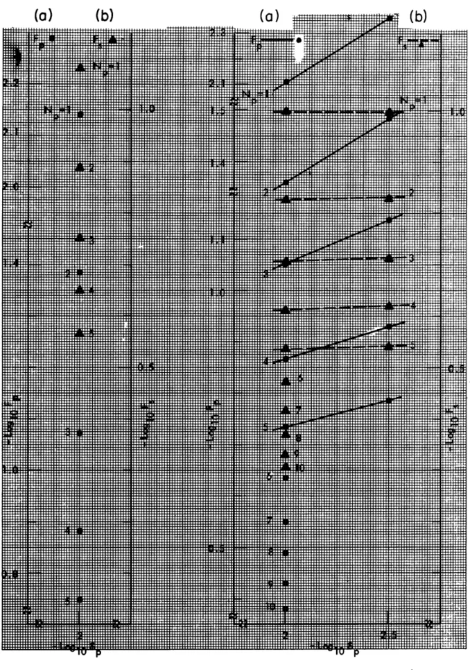
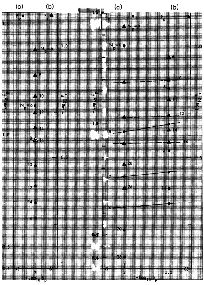
The design curves in Appendix B were derived from the main body of reference

designs 1-442. The range of filter parameters covered by these curves is exactly

the same as that covered by the tables, but the data are arranged somewhat

dif-ferently. Specifically, these curves were included to provide the filter designer with

first-order information about how the two cutoff frequencies vary with the ripple

heights and the parameter Np . For each class of filters of a particular order

essen-tially four different sets of design curves are presented. The first two sets present

plots of F and F vs 6 with fixed parameters N and 6 s The second two sets show

p s p s

how F and F vary with 6 while N and 6 are held constant. Within each set of

p s s p

curves Np is a parameter that is allowed to range over all of its prescribed values.

The arrangement of these curves within Appendix B is as follows. Initially the

curves are grouped according to filter order. That is, all design curves with N = 5

are presented first; next curves with N = 7 are displayed, and so on until curves

for the largest value of N have been presented. Within each grouping of a constant

N value the curves are arranged so that first plots of F and F vs 6S are

pre-p s s

sented with 6 fixed at its smallest value. Similar sets of curves are then

pre-P

sented with 6p increasingly incremented. After 6p has assumed all of its prescribed

values, plots of Fp and F vs 6p are presented with 6s fixed at progressively smaller

values. This arrangement, like that of the tables, provides a certain degree of

con-sistency in the variation of the cutoff frequencies within each grouping of curves, and hence enables the designer to solve his design problem more easily than would other-wise be possible.

Observation of a particular set of design curves, say, Fig. B-15a and B-15b, reveals that the parameters actually plotted, with the exception of Np, are the negative base 10

logarithms of those mentioned above. The reason for this is twofold. First, we

wanted to cover a large range of parameter values in a fairly precise manner and the

logarithmic scales made this possible. Second, we found that the design curves

when plotted on logarithmic scales exhibited essentially linear relations over many

of the prescribed parameter ranges. As a result, at least to a first

approxima-tion, a linear interpolation can be used between points on the curves to obtain a

design not explicitly catalogued.

Thus far the designs tabulated in Appendix A and displayed in Appendix B have

been specified only in terms of the four design parameters N, p, 6p, 6s, and the

two resulting cutoff frequencies F and F. For the designer wishing to imple- A

P 5

ment a particular design, a further specification, in terms of the filter unit

sample response, is needed. Appendix C presents the unit sample response for

each of the filters listed in Appendix A. Each filter is referenced by the same

call number in both appendices. The unit sample response of the zero-phase

specified by N+1 appropriate values.

Specifically, this unit sample response ho(n)

because the unit sample response h(n) of the linear phase filter is just that of the

zero-phase filter delayed by N samples it can be found directly from h (n) as

h(n) = h(n-N) n = 0, 1, ... , N. (12)

Thus the information in Appendices A-C serves to specify completely all of the

tabu-lated designs.

It will become evident from examination of the design curves and tables that only

filters with 6p

6 have been tabulated, and that with 6p = 6

designs were presented

only for values of Np , Ns.

The reason for this is that the reciprocal sets of filters

can easily be derived from those already tabulated by simple transformations that will

be described in Section VII.

15

VI. FORMULAS FOR ESTIMATING DESIGN PARAMETERS

Before discussing how the design curves and tables can be applied in practice it will

be helpful to present a few approximate relations that will facilitate their use. The

tabulated designs are uniquely specified by the four parameters N, Np, 6p, and 6s.

If the designer can formulate his problem in terms of these specifications he will be able to retrieve the solution from the tables and curves in a straightforward

manner. The design problem, however, is usually phrased in terms of Fp, Fs, 6p,

and 6s, or in terms of one of the cutoff frequencies, say Fp, the maximum

transi-tion bandwidth allowed, and 6p and 6 . In either case the designer must determine

appropriate values of N and Np to arrive at a particular solution. Although the

design curves and tables have been arranged to facilitate this procedure, it would be unnecessarily tedious to have to sort through the complete set of tabulated designs to arrive at one solution. What is needed is a set of simple, approximate expressions that relate the parameters N and Np to the others mentioned. By using these expressions, the designer can more readily decide just where in the set of design curves he should begin searching for a solution. Formulas 13 and 14, although yielding only rough estimates, have been found to be quite useful in this respect.

Herrmann6 has found the standard figure of merit D(N, Np, 6p, 6s) = 2N(Fs-F _{p )} to

be essentially independent of N and Np for values of N a 15. He has defined the quantity Do(6 _p 6s) for n ~ 15, and has empirically determined that

Do(6p, 6) = ZN(FS-Fp) 0. 55 (+log 1 0 6p) log1 0 6 + 0. 9 log1 0 + 2. 7. (13)

Furthermore, it has been found that

N F

P ,, P

(14)

N+ F +(0.5-F)

VII. USE OF DESIGN CURVES AND TABLES

The best way to 'illustrate how a designer might go about using the tables and

curves in Appendices A-C is to present examples of solutions for a few typical

designs.

7. 1 LOWPASS-FILTER DESIGN

Example 1

Consider the design of a linear-phase, equiripple, nonrecursive digital filter

spec-ified to have a magnitude frequency response that is flat to within 1% of unity for all

frequencies up to 0.193 and that has a stopband attenuation of at least -55 dB for

frequen-cies beyond 0. 360.

First, note that the frequencies must be specified in terms of the

normalized frequency variable F.

If f represents the analog frequency, and T is the

sampling period, then

F = fT. (15)

Once the frequencies have been properly prescribed, the other specifications must

be transcribed into the terminology used in the tables. For Example 1 they become F =

P

0. 193, F = 0. 360,

= 0.01, and

= 0.001.

Since no -55 dB filters were tabulated,

s p s

we decided to use a design with a -60 dB stopband attenuation. Use of the design curves

requires the additional conversion of some of these parameters into their base 10

log-arithms.

The resulting specifications are -log

F

= 0.714, -log

F

= 0.444,

-logl0 bp = 2, and -log0 6s = 3.

The next step is to use Eqs. 13 and 14 to see where in the set of design curves the

solution might be located.

From Eq. 13 the value of N is estimated as

approxi-mately 7. 5.

The nearest value for which designs have been tabulated is N = 7.

Using

N = 7 in Eq. 14 results in an estimated N of 4. 6.

We then restrict our attention to the

subset of design curves, Fig. B-11, in which N = 7 and

= 0. 01, or to the subset,

P

Fig. B-14, in which N = 7 and s = 0. 001. The solution is seen to lie on the curves with

N = 4. Specifically, one of the tabulated designs, denoted on the curves by ·

and

A

P

points, fits the specifications almost exactly.

The four parameters sufficient to uniquely specify this tabulated design are N = 7,

N = 4,

= 0.01, and

= 0. 001.

By using these four specifications, the exact design

p p s

solution may be found listed in Appendix A as filter 100, with cutoff frequencies F =

0. 19304, F = 0. 36032, and a transition bandwidth TBW = 0. 16728.

To complete the

s

solution of this design problem, it is only necessary for the designer to locate the

zero-phase filter unit sample response referenced under No. 100 in Appendix C and use

Eq. 12 to transform it into the unit sample response of a linear phase filter. It can be

verified from the design curves that this solution represents the lowest order solution

tabulated for the desired specifications.

17

Example 1 was somewhat oversimplified because the original specifications were chosen to match a tabulated design and hence to yield a straightforward solution of the problem. If a designer is faced with an initial specification of the two ripple tolerances

6 and 6s, the passband cutoff frequency F , and the maximum allowable transition

bandwidth TBWma_x , all randomly prescribed, there is no guarantee that a unique design

can be found from these tables. It may be necessary to make tradeoffs between several

tabulated designs to arrive at a compromise solution. Alternatively, if none of the catalogued designs are acceptable, the designer could use the design curves, tables, and the initial filter specifications to arrive at a set of suitable design parameters that would

yield a computer solution to his problem. Most of these concepts are illustrated in

Example 2.

Example 2

Consider the design of a nonrecursive, linear-phase, equiripple lowpass digital filter specified to have a maximum allowable passband ripple of 1% about unity out to a passband cutoff frequency of 0.1140. The stopband attenuation is prescribed to be at

least -60 dB, and the transition bandwidth must be 0. 0475 or less. With these

specifi-cations, it is understood that the lowest order filter satisfying these tolerances will be

the accepted solution. The design specifications of interest are the following.

F = 0. 1140, -logl_{1 0}F =0. 9431 p P Fs ~0. 1615, -log1 0 Fs 0.7918 6p 6.01I, -log1 0 6 p 2.0 p p 6s 0.001, -logo1 0 6s >3.0

Since a fairly narrow transition band has been specified, it is expected that the

design solution will be of a relatively high order. By using Eq. 13, the parameter N

is estimated as approximately 27. The nearest value of N for which designs have been

tabulated is N = 3 1. Also, with N = 3 1, Eq. 14 estimates Np as approximately equal to 8.

If we turn to Appendix B and locate Fig. B-36, with fixed parameters N = 31 and 6 =

P 0. 01, we find that a solution does indeed exist along the curves labeled Np = 8. None

of the tabulated designs exactly fits the specifications, however. The designer must

now choose one of the closest tabulated solutions or use the curves to predict the

param-eters that are necessary for a computer solution. The alternatives evident from these

curves are listed below as filter 356, or 357 (Appendix A).

Filter No. N N 6 6 F F TBW

Notice that filter 356 achieves all of the desired specifications except for F

and that

filter 357 achieves the specified Fp much more closely but has a stopband attenuation

of -70 dB.

The designer would probably settle for one of these designs, but if he

required Fp to be obtained more exactly, he could use the design curves to obtain the

necessary design specifications.

Specifically, from Fig. B-36a it is found that the value

of necessary to achieve an F = 0. 114 with N = 31, N = 8 and = 0.01 is =

-3

p

p

p

0. 5624 X 10

.

The resulting values for F and TBW may be found from Fig. B-36b

s

to be F

= 0. 1560 and TBW = 0. 0420.

Hence the computer solution could be specified

in terms of N = 31, N = 8, = 0.01 and = 0.0005624.

p p s

All of the designer's alternatives have not yet been exhausted. Additional designs

that fit the desired specifications can be found from Fig. B-40 where the fixed

param-eters are N = 31 and

s = 0. 00031623.

In particular, the curves in which N = 8 indicate

s p

that a solution exists for the specified F p, with 6 p= 0.008890, Fs = 0. 1605, and TBW =

0. 0465.

Hence a second computer solution exists with specifications N = 31, N

= 8,

p

6 = 0. 008890, and

s = 0. 00031623.

Still other possible solutions could be found by

p s

looking within the same set of curves at subsets where 6p and s assume other

satisfac-tory values.

Since the procedure has already been thoroughly demonstrated, these

solutions will not be found explicitly.

The remaining filter specification, which is the

unit sample response, can be found from Eq. 12 and Appendix C if the designer accepts

one of the tabulated filters or from the computer solution if he does not.

7.2 DESIGN OF FILTERS DERIVABLE FROM LISTINGS

As we have mentioned, designs have been tabulated only for values of 6p > 6

We

shall now present a method by which the reciprocal designs, 6p <

, can be obtained.

Consider the zero-phase, equiripple lowpass characteristic presented in Fig. 3. It is

prescribed to have certain design parameters Np, N

,

p , and

s, as well as a pair of

cutoff frequencies F and F s.

In terms of the filter unit sample response h (k), the

characteristic is defined as

N

Ho(F) =

ho(k) e

Fk

(16)

k=-N

In Fig. 4 a new frequency characteristic H(F) is formed by subtracting Ho(F) from

unity. This new characteristic is a highpass design defined by

H'

and

(17)

N

Ho(F

=

hho(k)

eZFk,

t k= -N

h

where the new unit sample response hho(k) is related to h (k) by

19

H (F)

=3

N =4

0.0

F

F

0.5

1.0

p

s

N

Ho(F)=

k=-N

ho (k)=O

6

>

8

h (k)

-J

rrFk

Ikl>

N

Fig. 3. Equiripple lowpass filter frequency response.

H'(F)

0.0

H' (F)=

Fhs Fhp

0.5

1.0

N

k

=-N

hho (k)

e

Fh=Fp; Fhp= FS

6hs=6p

hp=

s

Shs

>

hp

- ho(O)

k=r

hho(k)=

h

(k)

kO

0-ok)

LC

Fig. 4. Transformed highpass filter frequency response.

1 +6

1-6

P

+8

-6

C

F

1 +hp

1

-6hp

+Shs

-

hs

0

1

1

H (F) =I - HO(F

1 - ho(O) hho(k) =

k=0

k = -N ... , N; kS 0

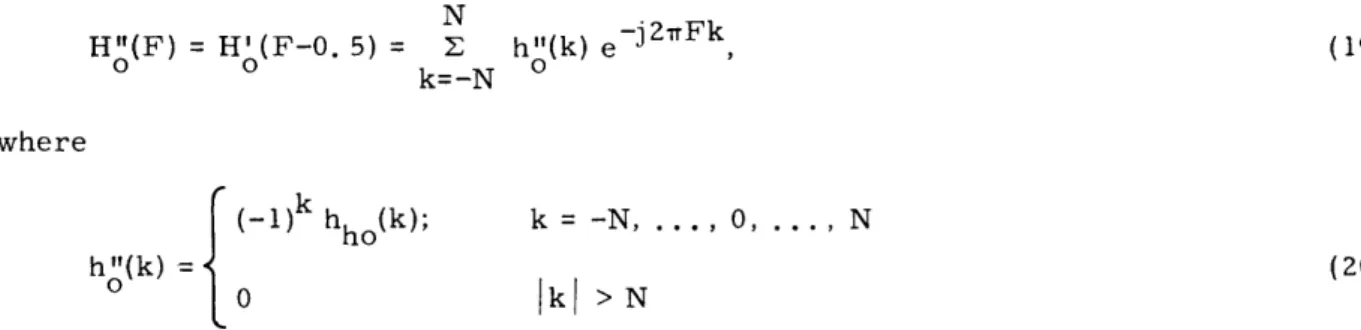
The final construction is shown in Fig. 5 where a third frequency characteristic H"(F) is formed by rotating H'(F) through a frequency shift AF = 0. 5. Since a

fre-0 0

quency shift of AF corresponds to multiplication of the unit sample response by a factor e 2 T F k , the new characteristic can be described by

N

~0

where

(19)

Ikl >N

Observation of Figs. 5 and 3 yields the desired results. Figure 5 represents a

zero-phase, equiripple, lowpass characteristic, but the new filter parameters N", N",

p s

6", 6", F", and F" are different from those of Fig. 3. Specifically, it is found that they

p

's

H"

(F)

1 +6"

P

₀

N" =4

P

0.0

F"

F"

0.5

1.0

p

s

F

H"

(F)=H (F-0.5)

o

N

-J2wFk

H"(F)=

h"(k)e

k -- N

kk==

hI(k)=(-1)k ho (k)

i -ho()

k=0

h"

(k) =

-ho(k)

k EVEN

,h

(k)

k

ODD

F;=

0.5-F$

F"

= 0.5

- F

6'=;

_P

_S

6 =6p

_P

8, <6"

P

Fig. 5. Transformed equiripple lowpass filter frequency response.

21

( 18)

(20)

-N" = N N" =Np (21) p s s p 6"

6

p

p

From Eqs. 20 and 18 the unit sample response corresponding to the characteristic of Fig. 5 is related to that of Fig. 3 by

1 - ho(0) k = 0

-h (k) k even

ho(k) = (24)

ho(k) k odd

0

Ikl >N

Equations 21-24 enable the designer to obtain solutions for values of 6" < 6" from values

p s

already tabulated. A specific example will serve to illustrate the concepts.

Example 3

Consider the design of an eleventh-order (N=5) linear-phase, equiripple, nonrecur-sive, lowpass digital filter with the specifications N" = 4, N" = 2, 6" = 0. 001, and 6" =

p s p s

0.01. Since 6" < 6"s', it is necessary to use the procedure just outlined. Equations 21

p s

and 22 give the specifications of the reciprocal filter as Np = 2, Ns = 4, 6 = 0.01, and 6 0.001. This filter, referenced as No. 22 in Appendix A, has cutoff frequencies Fp= 0.08568,

and Fs = 0.30889 which result in a transition bandwidth of TBW= 0.22321. Its unit sample

response is found from Appendix C to be ho(0)=0.360960841, ho(1)=0.275038898, ho(2) =

0. 101413727, ho(3) = -0. 015755489, ho(4) = -0. 034144104, ho(5) = -0. 012033358, and ho(k) = ho(-k); k = 1, 2, .... 5. By usingthese results and Eqs. 23 and 24, the solution to the design problem is a filter specified as N" = 4, N" = 2, 6" = 0.001, 5" = 0.01 with

cut-p s p s

off frequencies F" = 0. 19111, F" = 0.41432, the same transition bandwidth as before, and

p s

a unit sample response of h"(0) = 0.639039159, h"(l)=0.275038898, h"(2) = -0. 101413727, h"(3) =-0.015755489, h(4) =0.034144104, h"(5) =-0.012033358, and h"(k)=h"(-k); k = 1,

o 0 0 0 0

2, ... , 5. This unit sample response can again be shifted by Eq. 12 to obtain a linear-phase filter.

It is now evident why it was necessary to tabulate designs only for values of Np -< Ns when the parameters 6p and 6s were prescribed as equal. Designs with Np > Ns and 6 =

s can be obtained from the tabulated filters exactly as in this example.

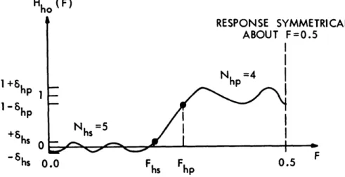
7.3 HIGHPASS FILTER DESIGN

the stopband and unity in the passband.

As in the case of a lowpass design, this ideal

characteristic is not realizable in practice. An equiripple approximation to this

high-pass characteristic is shown in Fig. 7.

The important specifications of this design are

MAGNITUDE

PASSBAN D

-1

STOPBAN

0.0

0.5

Fig. 6. Ideal highpass filter frequency response.

the two ripple heights, 6hs in the stopband and

hp in the passband; Nhs, the number

of stopband ripples; Nhp, the number of passband ripples; Fhs, the stopband cutoff

fre-quency; and Fhp, the passband cutoff frequency. Again N = Nhp + Nhs - 1, since the

ripples at F = 0.0 and F = 0. 5 are included in the specifications.

Each of the lowpass designs in Appendix A can be transformed into two highpass

designs of the same order that retain their equiripple characteristics and linear phase.

Consider again the zero-phase, equiripple, lowpass characteristic of Fig. 3.

The

per-tinent specifications are Np, N

I

p 6

I Fp, F

,

and the unit sample response h (k),

k = -N . .. , 0 . . .,N. One procedure (method 1) by which this characteristic can be

transformed to a highpass design has been demonstrated in conjunction with Fig. 4. The

highpass frequency characteristic Ho(F) is related to the lowpass characteristic Ho(F)

Hho (F)

1

+6hp

1

-6hs

0.0

'RI CAL

Nhs =5

Fh

Fhp

0.5

hs

hp

Fig. 7. Equiripple approximation to ideal highpass design.

23

1

F

1.0

-__-111_1_11-_-

·111- .1·-1-1--11

I-LI----C--I

I 1^1· _111_----··-_1--11I

Hho (F)

0

0.0

N

_hp

=

Fhs

Fhp

Hho(F)= H

(F-0.5)

N

-J

wFk

Hho(F) =

hho(k)e

k

=-N

ho(k)=(-1)k h(k)

1.0

F

Fhs =0.5-F ; Fhp=0.5-

Fp

Nhp

=N

;Nh

=N

p N

hs

s

bhs

=6s

;

hp

p

Shp >

Shs

Fig. 8.

Rotated equiripple highpass filter frequency response.

by Eq. 17 and the highpass design specifications are found from the lowpass

specifi-cations to be

hs

p'

Nhs

=

N

hs

p'

hs

p

Note

been

pass

F

= F

Nhp = N

6hp =

that method 1 is applicable only for values of 6hs > 6hp, since designs

tabulated only for values of 6 > 6 .

As before, it can be verified that the

is found from that of the lowpass filter by

unit sample response hho(k) is found from that of the lowpass filter by

(25)

(26)

(27)

have

hho(k) =

-ho(k)

O

k=O

k = -N, ... , N

k

O

Ik

> N

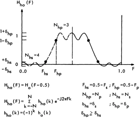
Another way (method 2) by which a tabulated lowpass design can be transformed into

a highpass filter is demonstrated in Fig. 8 where the lowpass characteristic of Fig. 3

(28)

1

+ hs

- hs

Fh =0.5 - Fs Fhp = 0.5 - F (29)

Nh =N N = N (30)

hs ' hp p

6

hs s' hp 6p (31)

and has a unit sample response hho(k) which is obtained from ho(k) as

(-1)

ho(k)

Ikl

N

hho(k) = kl > N (32)

Again, since lowpass designs have been tabulated only for 6p > 6s, method 2 is applicable

only when 6hp > 6hs. Another example will demonstrate the pertinent concepts.

Example 4

Consider the design of an 11 -order, linear-phase, equiripple, nonrecursive

highpass digital filter specified to have a magnitude frequency response with a stopband attenuation of at least -60 dB out to Fhs = 0. 112, and which is flat to within 1% of unity

beyond Fhp = 0.331. For this case, 6hs =0.001, hp = 0.01, and bhp > 6hs' so that

method 2 can be used.

The first step in the solution of the problem is to translate these highpass specifi-cations into an appropriate lowpass design so that the design curves and tables of Appen-dices A-C can be used. The resulting lowpass specifications found through Eqs. 29-31

are N = 5, 6 = 0.01, = 0.001, F = 0. 169, and F = 0. 388. By using Eq. 14, we

p s p s

estimate the parameter Np to be approximately 3.6. The next step is to locate the

spe-cified lowpass design on the design curves of Appendix B. In particular, Fig. B-3

reveals that the solution lies on the curves with N = 3, and that one of the tabulated P

filters meets the specifications almost exactly. This filter, No. 34 in Appendix A, has

design parameters N = 5, N = 3, 6 = 0.01, 6 = 0. 001, F =0.16920, and F =0.38818.

Transformation of these statistics back to the corresponding highpass design by Eqs. 29-31 yields a final design solution with parameters N, 6hp, and 6hs exactly as

specified, and cutoff frequencies Fhs = 0. 11182 and Fhp = 0. 33080. The unit sample

response corresponding to this zero-phase highpass solution is found from Eq. 32 and filter No. 34 listing in Appendix C to be hho(0)=0.528105617, hho(l) = -0. 302931309, hho(2) = -0.0Z2480451, hho(3) = 0.067077279, hho(4 ) = 0.010677606, hho(5) = -0.0168957 19, and hho(-k) =hho(k); k= 1, 2, ... , 5. Again, the unit sample response hh(k); k=0, 1, .... 2N associated with the corresponding linear-phase highpass filter can be found from

hh(k) = hho(k-N); k = 0, 1, 2N. (33)

In this example the original highpass specifications were chosen so that a solution

followed in a straightforward manner. If they had not been so chosen; that is, if they

25