Ground-based infrared mapping of H<sub>2</sub>O<sub>2</sub> on Mars near opposition

(1)

HAL Id: insu-02151733

https://hal-insu.archives-ouvertes.fr/insu-02151733

Submitted on 13 Jul 2019

HAL is a multi-disciplinary open access

archive for the deposit and dissemination of

sci-entific research documents, whether they are

pub-lished or not. The documents may come from

teaching and research institutions in France or

abroad, or from public or private research centers.

L’archive ouverte pluridisciplinaire HAL, est

destinée au dépôt et à la diffusion de documents

scientifiques de niveau recherche, publiés ou non,

émanant des établissements d’enseignement et de

recherche français ou étrangers, des laboratoires

publics ou privés.

opposition

Thérèse Encrenaz, Thomas K. Greathouse, Shohei Aoki, Frank Darden, Marco

Giuranna, François Forget, Franck Lefèvre, Franck Montmessin, Thierry

Fouchet, Bruno Bézard, et al.

To cite this version:

Thérèse Encrenaz, Thomas K. Greathouse, Shohei Aoki, Frank Darden, Marco Giuranna, et al..

Groundbased infrared mapping of H2O2 on Mars near opposition. Astronomy and Astrophysics

-A&A, EDP Sciences, 2019, 627, A 60 (10p.). �10.1051/0004-6361/201935300�. �insu-02151733�

(2)

Astronomy

_&

Astrophysics

A&A 627, A60 (2019)

https://doi.org/10.1051/0004-6361/201935300 © T. Encrenaz et al. 2019

Ground-based infrared mapping of H

2

O

2

on Mars near opposition

T. Encrenaz

1

_{, T. K. Greathouse}

2

_{, S. Aoki}

3

_{, F. Daerden}

3

_{, M. Giuranna}

4

_{, F. Forget}

5

_{, F. Lefèvre}

6

_{, F. Montmessin}

6

_,

T. Fouchet

1

_{, B. Bézard}

1

_{, S. K. Atreya}

7

_{, C. DeWitt}

8

_{, M. J. Richter}

9

_{, L. Neary}

3

_{, and S. Viscardy}

3

1_{LESIA, Observatoire de Paris, CNRS, PSL University, Sorbonne Université, Sorbonne Paris Cité, 92195 Meudon, France} e-mail: therese.encrenaz@obspm.fr

2_{SwRI, Div. 15, San Antonio, TX 78228, USA}

3_{Planetary Aeronomy Team, BIRA-IASB, 3 Avenue Circulaire, 1180 Brussels, Belgium} 4_{IAPS–INAF, Via del Fosso del Cavaliere 100, 00133 Rome, Italy}

5_{LMD, IPSL, 75252 Paris Cedex 05, France} 6_{LATMOS, IPSL, 75252 Paris Cedex 05, France}

7_{Climate and Space Sciences and Engineering Department, University of Michigan, Ann Arbor, MI 48109-2143, USA} 8_{SOFIA Science Center, Ames Research Center, Moffett Field, Mountain View, CA 94035, USA}

9_{Department of Physics, University of California Davis, CA 95616, USA} Received 18 February 2019 / Accepted 11 May 2019

ABSTRACT

We pursued our ground-based seasonal monitoring of hydrogen peroxide on Mars using thermal imaging spectroscopy, with two observations of the planet near opposition, in May 2016 (solar longitude Ls = 148.5◦_{, diameter = 17 arcsec) and July 2018 (Ls = 209}◦_, diameter = 23 arcsec). Data were recorded in the 1232–1242 cm−1_{range (8.1 µm) with the Texas Echelon Cross Echelle Spectrograph} (TEXES) mounted at the 3 m Infrared Telescope Facility (IRTF) at the Mauna Kea Observatories. As in the case of our previous analyses, maps of H2O2 were obtained using line depth ratios of weak transitions of H2O2 divided by a weak CO2line. The H2O2 map of April 2016 shows a strong dichotomy between the northern and southern hemispheres, with a mean volume mixing ratio of 45 ppbv on the north side and less than 10 ppbv on the south side; this dichotomy was expected by the photochemical models developed in the LMD Mars Global Climate Model (LMD-MGCM) and with the recently developed Global Environmental Multiscale (GEM) model. The second measurement (July 2018) was taken in the middle of the MY 34 global dust storm. H2O2 was not detected with a disk-integrated 2σ upper limit of 10 ppbv, while both the LMD-MGCM and the LEM models predicted a value above 20 ppbv (also observed by TEXES in 2003) in the absence of dust storm. This depletion is probably the result of the high dust content in the atmosphere at the time of our observations, which led to a decrease in the water vapor column density, as observed by the PFS during the global dust storm. GCM simulations using the GEM model show that the H2O depletion leads to a drop in H2O2, due to the lack of HO2radicals. Our result brings a new constraint on the photochemistry of H2O2in the presence of a high dust content. In parallel, we reprocessed the whole TEXES dataset of H2O2measurements using the latest version of the GEISA database (GEISA 2015). We recently found that there is a significant difference in the H2O2line strengths between the 2003 and 2015 versions of GEISA. Therefore, all H2O2volume mixing ratios up to 2014 from TEXES measurements must be reduced by a factor of 1.75. As a consequence, in four cases (Ls around 80◦_{, 100}◦_{, 150}◦_{, and 209}◦_{) the H}₂_O₂ _{abundances show contradictory values between different Martian years. At} Ls = 209◦_{the cause seems to be the increased dust content associated with the global dust storm. The inter-annual variability in the} three other cases remains unexplained at this time.

Key words. planets and satellites: composition – planets and satellites: terrestrial planets – infrared: planetary systems – infrared: general

1. Introduction

Hydrogen peroxide H2O2 is known to be a key molecule in

the photochemistry of the Martian atmosphere. At the time of the Viking exploration, this molecule was suggested as the potential oxidizer responsible for the absence of organics on

the surface of Mars (Oyama & Berdahl 1977). The presence

of H2O2 was expected, with volume mixing ratios (vmr) of

a few parts per billion at most, on the basis of

photochemi-cal models (Krasnopolsky 1993, 2009; Clancy & Nair 1996;

Atreya & Gu 1995). Hydrogen peroxide was first detected from

the ground in the submillimeter range (Clancy et al. 2004),

then it was repeatedly mapped with ground-based imaging spec-troscopy in the thermal infrared range to study its seasonal cycle, using the Texas Echelon Cross Echelle Spectrograph (TEXES) mounted on the Infrared Telescope Facility (IRTF)

at the Mauna Kea Observatories (Encrenaz et al. 2004,2012,

2015). This dataset has been compared with photochemical

mod-els developed in the frame of the Mars Global Climate Model of the Laboratoire de Météorologie Dynamique (LMD-MGCM, Forget et al. 1999), and has been shown to favor heterogeneous

chemistry with respect to gas-phase chemistry (Lefèvre et al.

2008).

We took advantage of two favorable oppositions of Mars, in

May 2016 and July 2018, to obtain new maps of H2O2 at high

spatial resolution. Then we were able to observe Mars in the middle of the M34 global dust storm, which gave us an

unex-pected opportunity to study the behavior of H2O2in the presence

of a large dust content. While the H2O2map of May 2016 was

in full agreement with the expectations, the H2O2abundance in

July 2018 was surprisingly low. The present paper reports these two new observations.

A60, page 1 of10

Open Access article,published by EDP Sciences, under the terms of the Creative Commons Attribution License (http://creativecommons.org/licenses/by/4.0), which permits unrestricted use, distribution, and reproduction in any medium, provided the original work is properly cited.

(3)

In the present analysis, we used the GEISA 2015 spectro-scopic database. We found that there is a significant difference

between the H2O2 line strengths reported in GEISA 2015 and

those of GEISA 2003, used for our earlier analyses, with the 2015 values being higher by a factor close to 1.75. This problem is

addressed in more detail in Sect.4.1. As a result, we recalibrated

the whole H2O2dataset using the new GEISA values.

In Sect.2we describe the observation of May 2016 and its

comparison with the global climate models. In Sect.3we present

the results of the July 2018 observations. In Sect. 4 we first

present the whole H2O2 dataset using the GEISA 2015

spec-troscopic database. Then we analyze the discrepancy observed between the TEXES data of July 2018 and the models, and we propose an interpretation associated with the high dust content of the MY 34 global dust storm. Finally, we discuss the whole

H2O2 dataset and we note several cases of inter-annual

varia-tions, which remain unexplained at this time. Our conclusions

are summarized in Sect.5.

2. Ls = 148.5◦_{(May 2016)}

2.1. TEXES observations

The Texas Echelon Cross Echelle Spectrograph (TEXES) is an imaging spectrometer operating between 5 and 25 µm that combines a high resolving power (above 80 000 at 8 µm in the high-resolution mode) and a good spatial resolution (about 1 arcsec). A full description of the instrument can be found in Lacy et al. (2002). We used the instrument at the 3 m Infrared Telescope Facility (IRTF) at the Mauna Kea Observa-tories (Hawaii). As we did in the case of our first observation in

2003 (Encrenaz et al. 2004,2012), we used the 1230–1236 cm−1

spectral range (8.09–8.13 µm) where weak transitions of CO2

and H2O2are present.

Data were recorded on May 7, 2016, between 08:00 and

9:00 UT. The solar longitude (Ls) of Mars was 148.5◦_{. The}

diam-eter of the planet was 17.0 arcsec and its illumination factor was 98.8%. We used a 1.1 × 8 arcsec slit, aligned along the celes-tial north-south axis, and we stepped the telescope by 0.5 arcsec in the west-east direction between two successive integrations in order to map the Martian disk. Because the slit length was much smaller than the diameter of Mars, we co-added three succes-sive scans corresponding to the southern hemisphere, the central region, and the northern hemisphere of the planet. The total observing time was about 45 min. The mean longitude of the

sub-Earth point during the observation was 75◦_W.

The disk-integrated spectrum is shown in Fig.1. The Doppler

shift at 1234 cm−1 _{is + 0.031 cm}−1_{. The TEXES data cubes are}

calibrated using the radiometric method commonly used for sub-millimeter/millimeter astronomy, which is described in detail in Lacy et al.(2002).

As in the case of our previous observations, we chose weak

transitions of H2O2 and CO2, well isolated from telluric lines.

Using the GEISA 2015 database (which is in agreement with the HITRAN 2016 dabase), we selected the same parame-ters as were used for our first observation in June 2003: the

H2O2 doublet of the ν6 band at 1234.011 cm−1 (I = 2.650 ×

10−20_{cm molec}−1_{, E = 267.926 cm}−1_{) and 1234.055 cm}−1 _{(I =}

2.82 × 10−20_{cm molec}−1_{, E = 261.164 cm}−1_{), which is close}

to a weak CO2 isotopic (628) transition at 1233.929 cm−1

(I = 4.13 × 10−27_{cm molec}−1_{, E = 88.357 cm}−1_{). Figure}₁ _shows

the disk-integrated spectrum of Mars between 1232.5 and

1234.2 cm−1_{, compared with the atmospheric transmission, as}

observed by the TEXES instrument, and a nominal synthetic

0.7 0.75 0.8 0.85 0.9 0.95 1 1.05 1232.6 1232.8 1233 1233.2 1233.4 1233.6 1233.8 1234 1234.2 Normalized radiance Wavenumber (cm-1) l i i CO2 CO2 CO2 l l H2O2 l l l l l l l Atm CO2 Atm Atm CO2 Atm Atm

__ TEXES

__ Model CO2 __Model H2O2

__Atm.transmission

Fig. 1. Thick black line: spectrum of Mars between 1232.6 and

1234.2 cm−1_{, integrated over the Martian disk, recorded on May 7,} 2016 (Ls = 148.5◦_{, normalized radiance). Synthetic spectra of Mars:} CO2 alone (blue), H2O2alone with H2O2/CO2= 100 ppbv (red). Thin black line (in absolute units shifted by −0.05): transmission from the terrestrial atmosphere, as measured by the TEXES instrument. “Atm” indicates terrestrial absorption.

spectrum calculated for a H2O2volume mixing ratio of 100 ppbv,

indicating the positions of the CO2and H2O2transitions.

The H2O2 mixing ratio was estimated from the mean ratio

of the line depths of the H2O2 doublet divided by the CO2line

depth. As discussed in earlier papers (in particular, seeEncrenaz

et al. 2015), this first-order method minimizes the uncertainties associated with the surface and atmospheric parameters, as well as the effect of the airmass factor. We checked the linearity of the

H2O2/CO2line depth ratio with respect to the H2O2volume

mix-ing ratio for a wide range of thermal profiles and for air masses as high as 5.0. This study has shown that the maximum departure is

10% for an airmass of 5.0 (Encrenaz et al. 2015). As in our

previ-ous studies, our mixing ratios, expressed by volume, are derived relative to carbon dioxide.

In the case of CO2, we checked the consistency of our results

by mapping several CO2 lines whose intensities are

compara-ble to that of the 1233.928 cm−1_{transition. This comparison has}

shown that the 1233.929 cm−1 _CO₂ _{transition is polluted by an}

instrumental artifact, with a spike appearing occasionally very close to the line center. We checked that this artifact was not present in our previous observation in June 2003; however, it also appeared on July 6, 2018, as we discuss below. For this

rea-son, we used another CO2transition of comparable intensity at

1233.203 cm−1 _{(I = 4.16 × 10}−27_{cm molec}−1_{, E = 100.137 cm}−1₎

as a proxy of this line.

Figure2 shows the maps of the continuum radiance

(mea-sured at 1233.95 cm−1_{), the CO}₂ _{line depth (measured for the}

1233.203 cm−1 _{transition), and the mean value of the depths of}

the H2O2lines at 1234.011 and 1234.055 cm−1_{. For comparison,}

Fig.3 shows the maps of the surface temperature and the

tem-perature contrast T(z = 1km) – Ts for the same season and the same geometry, derived from the LMD Mars Climate Database

(MCD,Forget et al. 1999). The continuum radiance is at its

max-imum at the center of the scene, as expected since the sub-Earth point is in the early afternoon, close to the subsolar point; the strong decrease observed in the TEXES map toward the edge is primarily due to the increasing airmass of the colder atmosphere.

The CO2line depth map measured by TEXES is the combination

of three factors: (1) the surface pressure (hence the topography), A60, page 2 of10

(4)

T. Encrenaz et al.: Infrared mapping of H2O2on Mars near opposition H2 O2 line de pt h CO2 line de pt h Co nt inuum ra di anc e (e rg /s /c m 2/s r/ cm -1) Continuum radiance (1234.95 cm-1₎ CO2 line depth (1233.20 cm-1₎ H2O2 line depth (1234.01 & 1234.05 cm-1₎

Fig. 2.Maps of the continuum radiance at 1233.95 cm−1_{(top), the CO}₂

line depth at 1233.203 cm−1_{(middle), and the mean value of the H}₂_O₂ line depths at 1234.011 and 1234.055 cm−1_{(bottom), recorded on May 7,} 2016 (Ls = 148.5◦_{). The Martian north pole is at the top of the figure. The} subsolar point is shown (white dot).

Fig. 3.Synthetic maps of (left) the surface temperature, and (right) the

temperature contrast T(z=1km) – Ts, for the seasonal range Ls = 150– 180◦_{. The maps are from the Mars Climate Database (}_{Forget et al. 1999}_).

(2) the temperature contrast between the atmosphere and the sur-face, and (3) the airmass. The airmass effect explains why the

observed CO2 line depth is highest on the northern and

west-ern limbs of the planet. The observed CO2 line depth is low in

the southeast part of the map because of the lower temperature

contrast and the higher elevation. The H2O2 line depth is also

affected by the same effects.

H2 O2 /C O2 mi xi ng ra. o (ppb v) H2 O2 /C O2 mi xi ng ra. o (ppb v) H2 O2 /C O2 mi xi ng ra. o (ppb v) TEXES LMD-‐MGCM GEM-‐Mars

Fig. 4. Top: map of the H2O2/CO2 volume mixing inferred from the

H2O2/CO2 line depth ratio, using the transitions shown in Fig.2. The conversion factor between the H2O2vmr and the H2O2ldr is the follow-ing: vmr = 45.0/0.13 ldr (see text, Sect.2.2). The subsolar point is shown as a white dot. Middle: synthetic map of the H2O2vmr for Ls = 145–150◦ as predicted by the LMD-MGCM (Forget et al. 1999). Bottom: same synthetic map, generated by the GEM model (Daerden et al. 2019). The bright spots observed on the TEXES map at the limb may be an artifact, or due to the low signal near the limb, implying a larger error bar.

Figure 4 shows a map of the H2O2/CO2 line depth ratio

(ldr), using the transitions shown in Fig.2, compared with two

maps of the H2O2 volume mixing ratio, as predicted by the

LMD-MGCM and the Global Environmental Multiscale (GEM) models. The three maps show a very good qualitative agree-ment, and all show a clear dichotomy between the northern and southern hemispheres.

2.2. Data interpretation and modeling

On the basis of the north-south dichotomy shown by our map

(Fig.3), we integrated the spectra separately in the northern and

southern hemispheres, and we compared the integrated spectra in these two regions with synthetic models. The west

longi-tude range was 75◦_{± 80}◦ _{in both cases. The latitude range was}

(8◦_N–90◦_{N) in the northern hemisphere and (50}◦_S–8◦_{N) in the}

southern hemisphere. We used the atmospheric parameters (sur-face pressure, sur(sur-face temperature, and thermal profile) inferred

from the MCD (Forget et al. 1999). For the northern and southern

hemispheres the mean temperatures were 275 and 255 K at the surface, 225 and 218 K at z = 1 km, 197 and 192 K at z = 10 km, A60, page 3 of10

(5)

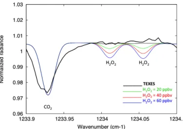
Fig. 5. Bold dark line: spectrum of Mars between 1233.9 and 1234.1 cm−1_{, integrated over the northern hemisphere of the planet,} recorded on May 7, 2016 (Ls = 148.5Å, normalized radiance). Thin lines: synthetic models, calculated using the atmospheric parameters described in Sect.2.2: Black: H2O2= 0 ppbv; green: H2O2= 20 ppbv; red: H2O2= 40 ppbv; blue: H2O2= 60 ppbv. The best fit is obtained for a value of 45 ppbv. The spectral resolution of the models is 0.024 cm−1_.

respectively, and 155 K for both hemispheres above z = 50 km. The mean surface pressure was 5.5 and 3.6 mbar for the northern and southern hemispheres, respectively. We then used the CO2 transitions to check the consistency of these parameters, and we

used them to model the H2O2transitions. Calculations show that

for all transitions the lines are mostly formed in the lower tropo-sphere, within the first ten kilometers above the surface. From the synthetic spectra we derived the following relationship between

the H2O2volume mixing ratio and the H2O2/CO2line depth ratio

corresponding to the transitions shown in Fig.2:

H2O2vmr(ppbv) = 45.0/0.13 × (H2O2/CO2)ldr.

Our synthetic spectra were modeled using spectroscopic data

extracted from the GEISA 2015 molecular database (

Jacquinet-Husson et al. 2016). In the case of the CO2 broadening

coef-ficient, we used the values quoted by Pollack et al.(1993) and

references therein. As in our previous analyses, we assumed for

H2O2 a constant mixing ratio as a function of altitude. This

assumption is actually required to infer the H2O2volume mixing

ratio from the H2O2/CO2 line depth ratio. According to

photo-chemical models, the H2O2 cutoff is expected to occur above

an altitude of about 10 km near aphelion (northern spring and summer) and about 30 km around perihelion (southern spring

and summer), and the H2O2 mixing ratio is more or less

con-stant below this threshold (Encrenaz et al. 2012). Because the

H2O2and CO2 lines are weak, they are formed in the first

kilo-meters above the surface. We thus expect the assumption of a

constant H2O2 mixing ratio to have a minor influence on our

results. Figures5 and6 show the integrated TEXES spectra in

the northern and southern hemispheres, respectively. From the

comparison with synthetic spectra, we infer a mean H2O2 vmr

of 45 ± 10 ppbv (2σ error bars) in the northern hemisphere, and a 2σ upper limit of 10 ppbv in the southern hemisphere, in good

agreement with the climate model predictions (Fig.4).

3. Ls = 209◦_{(July 2018)}

Our observing run took place between July 6 and July 14, 2018

(Ls = 206–211◦_{). At that time, the planet was surrounded by a}

Fig. 6. Bold dark line: spectrum of Mars between 1233.9 and

1234.1 cm−1_{, integrated over the southern hemisphere of the planet,} recorded on May 7, 2016 (Ls = 148Å, normalized radiance). Thin lines: synthetic models, calculated using the atmospheric parameters described in Sect.2.2: Black: H2O2= 0 ppbv; green: H2O2= 20 ppbv; red: H2O2= 40 ppbv; blue: H2O2= 60 ppbv. H2O2is undetected, with a 2σ upper limit of 10 ppbv. The poor fit of the CO2line in the southern hemisphere is due to the occasional presence of a spike near the line center. The spectral resolution of the models is 0.024 cm−1_.

Table 1. Summary of TEXES observations of Mars in July 2018.

Date Time SEP SSP Frequency

of obs. (UT) W long. W long. range (cm−1₎

2018/07/06 14:02:31 101.0 118.7 1232–1238

2018/07/10 13:30:57 57.8 72.7 1232–1238

2018/07/11 10:27:22 5.0 19.2 1237–1242

2018/07/11 13:21:45 46.4 60.6 1232–1238

2018/07/14 10:25:16 338.1 350.2 1232–1238

strong global dust storm that affected the temperature profile and the dust content significantly. The Martian diameter ranged from 21.9 to 23.2 arcsec, with an illumination factor above 97.7%. Two spectral intervals were recorded, at 1232–1238 and at 1237–

1242 cm−1_{. The mean Doppler shift was +0.024 cm}−1_{. Data were}

recorded in the same way as described above for the May 2016 observations. The observing time for a full map was about one

hour. The observations are summarized in Table1.

3.1. The 1234 cm-1region

Figure 7 shows the four spectra recorded in July 2018 in the

1233.6–1234.5 cm−1 _{spectral range. A comparison with Fig.}₁

shows that the CO2line depths are weaker than in our May 2016

observation. This is the effect of the global dust storm, which decreases the atmospheric temperature gradient and the temper-ature contrast between the atmosphere and the surface. It can

be seen that the H2O2doublet, easily identified in the northern

hemisphere in our May 2016 observation, is undetected. We first selected the disk-integrated spectrum of July 11,

2018. To model the H2O2spectrum, we used a temperature

pro-file extracted from the MCD for a high dust content. This propro-file assumes a temperature of 248 K at an altitude of 1 km, an isothermal profile at 245 K between 1 and 20 km, and a tem-perature of 200 K at 50 km. The surface pressure was 5 mbar, A60, page 4 of10

(6)

T. Encrenaz et al.: Infrared mapping of H2O2on Mars near opposition 0.2 0.3 0.4 0.5 0.6 0.7 0.8 0.9 1 1.1 1233.6 1233.7 1233.8 1233.9 1234 1234.1 1234.2 1234.3 1234.4 1234.5 Normalized radiance Wavenumber (cm-1) July 6 July 10 July 11 July 14 l l l l l l l CO2 Atm Atm CO2 H2O2 CO2 ___ TEXES data doublet ___ Synthetic model, H2O2= 60 ppbv CO2

Fig. 7.Black lines: normalized disk-integrated spectra of Mars between

1233.6 and 1234.5 cm−1_{, recorded on July 6, 10, 11, and 14, 2018, shifted} vertically by 0.0, −0.1, −0.2, and −0.3, respectively. In the July 6 spec-trum, a spike was present at 1233.93 cm−1_{, at the position of the CO}₂ line, and has been removed. Red line: synthetic model, calculated using the atmospheric parameters described in Sect.3.1, with H2O2= 60 ppbv, shifted by −0.5. The spectral resolution of the models is 0.014 cm−1_.

0.96 0.97 0.98 0.99 1 1.01 1233.9 1233.95 1234 1234.05 1234.1 1234.15 Normalized radiance Wavenumber (cm-1) _____ TEXES _____ H2O2= 0 ppbv _____ H2O2= 30 ppbv _____ H2O2= 60 ppbv

Fig. 8.Black line: normalized disk-integrated spectra of Mars between

1233.60 and 1234.50 cm−1_{, recorded on July 11, 2018. Colored lines} indicate the synthetic models, calculated using the atmospheric param-eters described in Sect. 3.1: H2O2= 0 ppbv (green), 30 ppbv (red), and 60 ppbv (blue). H2O2 is undetected. The spectral resolution of the models is 0.014 cm−1_.

and we adjusted the surface temperature at 251 K in order to

fit the CO2transition at 1233.929 cm−1_{. During southern spring,}

Fig.8shows a comparison of our spectrum with synthetic

mod-els, calculated for different values of the H2O2vmr, assuming a

constant mixing ratio. It can be seen that the noise level of the TEXES spectrum does not allow us to derive a significant upper limit.

In order to improve our H2O2 upper limit, we co-added the

four spectra recorded around 1234 cm−1 _{in July 2018. Because}

of the presence of an artifact near the CO2line on July 6 (also

present in 2016, as mentioned above), we removed the July 6

spectrum for the summation below 1233.95 cm−1_{, and we kept}

the four spectra above this frequency. Figure9shows the

result-ing spectrum, corrected for the slope variations shown in Figs.7

and8. To do so, we used two straight lines of different slopes,

below and above 1234.05 cm−1_{, in order to remove the slope}

difference in the continuum (see Fig. 8). We estimate the 3σ

0.97 0.975 0.98 0.985 0.99 0.995 1 1.005 1.01 1233.9 1233.92 1233.94 1233.96 1233.98 1234 1234.02 1234.04 1234.06 1234.08 1234.1 Normalized radiance Wavenumber (cm-1) 1233.9&&&&&&&&&&&&&&&&1233.95&&&&&&&&&&&&&&&&&&1234.0&&&&&&&&&&&&&&&&&1234.05&&&&&&&&&&&&&1234.1& & & & & & &&&Wavenumber&(cm51)&&&&&&&&&&&&&&&&&&&&&&&&&&&&&&&&&&&&&&&&&&&&&

&&l&&&&&&&&&&&&&&&&&&&&&&&&&&&&&&&&&&&&&&&&&&&&&&&&&&&&&&&&&&&&&&&&&&&l&

_____ TEXES _____ H2O2= 0 ppbv

_____ H2O2= 15 ppbv _____ H2O2= 30 ppbv

Fig. 9. Black line: averaged disk-integrated spectra of Mars between

1233.90 and 1234.10 cm−1_{, obtained from the summation of the four} spectra shown in Fig.7. For the July 6 spectrum, a spike appeared at the position of the CO2line at 1233.93 cm−1, so the averaged CO2line was obtained from the summation of the three other spectra. Synthetic models were calculated using the atmospheric parameters described in Sect.3.1, with H2O2= 0 ppbv (green line), 15 ppbv (red line), and 30 ppbv (blue line). H2O2 is undetected, with a 2σ upper limit of 15 ppbv. The spectral resolution of the models is 0.014 cm−1_.

peak-to-peak fluctuations of the spectrum to be 0.003.

Compari-son with the models shows that a H2O2volume mixing ratio of

15 ppbv corresponds to a line depth of 0.002. We thus derive

from the 1234 cm−1_{data a 2σ upper limit of 15 ppbv.}

We wondered whether the H2O2 distribution over the disk

might be very inhomogeneous, as observed in May 2016. For this

reason, we mapped the line depths of CO2and H2O2as we did

for our previous observations. Figure10shows, as an example,

the maps of the continuum radiance at 1233.98 cm−1_{, the CO2}

line depth at 1233.93 cm−1_{, and the line depth of the H}₂_O₂_line

at 1234.05 cm−1_{corresponding to the map of July 11, 2018. The}

H2O2line depth map shows that the H2O2abundance is close to

zero everywhere on the Martian disk.

For comparison, Fig.11shows the synthetics maps of the

sur-face temperature and the temperature contrast T(z = 1km) – Ts for two different scenarios, the normal case and the dusty case (MY 25), derived from the LMD-MGCM under the same observing conditions. The continuum radiance observed in

July 2018 (Fig.10) exhibits lower values than in Fig.2, with a

maximum that is two times lower. This is due to the lower day-time surface temperature, and to a stronger contribution from the

dust-laden atmosphere. The CO2line depth is very different from

that in Fig.2, which probably reflects a different distribution of

the dust at this period. During the global dust storm, the dust opacity was high at every longitude and latitude, except north of

about 40◦_{N (}_{Kass et al. 2018}_{). It is thus likely that our planetary}

averaged spectra are mostly sensitive to the less dusty middle and high northern latitudes.

3.2. The 1241 cm–1region

In the 1241 cm−1_{spectral range, a single map was obtained on}

July 11, 2018. As in many previous measurements, we used the

H2O2doublet around 1241 cm−1_{, but this time with the GEISA}

2015 database. The H2O2doublet appears at 1241.533 cm−1_{(I =}

3.60 × 10−20_{cm molec}−1_{, E = 155.502 cm}−1_{, and at 1241.613 cm}−1

(I = 3.37 × 10−20_{cm molec}−1_{, E = 163.185 cm}−1_{). It brackets a}

weak (unresolved) CO2 doublet (1241.574 and 1241.580 cm−1,

(7)

CO2 line depth -‐1₎ C O2 line d ep th Con$nuum Radiance (1233.90 cm-‐1₎ H2O2 line depth (1234.05 cm-‐1₎ H 2 O2 line d ep th C on $n uu m Rad ian ce ( er g/ s/ cm 2/s r/ cm -‐1) (1233.93 cm

Fig. 10. Maps of the continuum radiance at 1233.90 cm−1 _{(top), the}

CO2 line depth at 1233.93 cm−1 (middle), and the H2O2 line depth at 1234.05 cm−1_{(bottom), corresponding to the 1234 cm}−1_{map of July 11,} 2018. H2O2 is undetected. The Martian north pole is at the top of the figure. The subsolar point is shown as a white dot.

I= 5.15 × 10−27cm molec−1, E = 664.59 cm−1). As mentioned

above, the intensities of the H2O2 lines are higher than the

GEISA 2003 values by a factor of about 1.75. The implications

of this change are discussed in Sect.4.

Figure12shows the disk-integrated spectrum of Mars

corre-sponding to this map, in the 1241.5–1241.65 cm−1_{spectral range.}

As in the previous case, there is no clear detection of the H2O2

doublet. The strong fluctuations of the continuum in the

imme-diate vicinity of the H2O2doublet, and the short spectral interval

available for measuring it, make the comparison with synthetic models more difficult than in the previous case. We tentatively estimate the 3σ peak-to-peak continuum fluctuations to be 0.004.

A H2O2volume mixing ratio of 10 ppbv corresponds to a depth

of 0.002. We thus derive a 2σ upper limit of 15 ppbv for the

mean H2O2vmr over the Martian disk.

As in the case of the 1234 cm−1 _{data, we mapped the}

line depths of CO2 and H2O2 to search for possible

varia-tions in the H2O2 abundance over the disk. Figure 13 shows

the maps of the continuum radiance at 1241.60 cm−1_{, the CO2}

line depth at 1241.62 cm−1_{, and the line depth of the H}

2O2line

at 1241.57 cm−1_{. As in the previous case, there is no evidence}

of any enhancement of the H2O2 abundance over the Martian

disk.

Fig. 11.Synthetic maps of (top) the surface temperature, and (bottom)

the temperature contrast T(z = 1km) – Ts, assuming the standard scenario (left) and the MY 25 dust scenario. The seasonal range is Ls = 180–210◦_{. The maps are extracted from the Mars Climate Database}

(Forget et al. 1999). 0.975 0.98 0.985 0.99 0.995 1 1.005 1241.5 1241.52 1241.54 1241.56 1241.58 1241.6 1241.62 1241.64 Normalized radiance Wavenumber (cm-1) _____ TEXES _____ H2O2= 0 ppbv _____ H2O2= 10 ppbv _____ H2O2= 20 ppbv

Fig. 12.Black line: normalized disk-integrated spectra of Mars between

1241.50 and 1241.65 cm−1_{, recorded on July 11, 2018. The synthetic} models are calculated using the atmospheric parameters described in Sect. 3.1: Green: H2O2= 0 ppbv; red: H2O2= 10 ppbv; blue: H2O2= 20 ppbv. H2O2is undetected, with a 2σ upper limit of 15 ppbv. The spectral resolution of the models is 0.014 cm−1_.

3.3. Validity of the radiative transfer code in the case of dusty conditions

In all our previous analyses, we used a line-by-line radiative transfer without scattering, which was found to be reliable for calculating the thermal infrared spectrum of Mars under nor-mal dust conditions. In the case of our July 2018 observations, we needed to check the validity of our code in the condi-tions of a global dust storm. We used a radiative transfer code A60, page 6 of10

(8)

T. Encrenaz et al.: Infrared mapping of H2O2on Mars near opposition Con$nuum (1241.60 cm-‐1₎ CO₂ line depth (1241.62 cm-‐1₎ H2O2 line depth (1241.57 cm-‐1₎ H 2 O2 line d ep th C O2 line d ep th C on $n uu m Rad ian ce ( er g/ s/ cm 2/s r/ cm -‐1)

Fig. 13. Maps of the continuum radiance at 1241.60 cm−1 _{(top), the}

CO2 line depth at 1241.62 cm−1 (middle), and the H2O2 line depth at 1241.57 cm−1_{(bottom), corresponding to the 1241 observation of July} 11, 2018. H2O2is undetected. The Martian north pole is at the top of the figure. The subsolar point is shown (white dot).

including multiple scattering (Aoki et al. 2018) and we modeled

the 1241.52–1241.63 cm−1 _{spectral range, including the H}₂_O₂

doublet and the CO2line found in this range, assuming a global

dust scenario similar to MY 25 (Daerden et al. 2019). We have

assumed H2O2 and CO2 to be uniformly mixed. Results are

shown in Fig.14. In this model the dust opacity is equal to 3.5–4

in the latitude range (30N–60S), corresponding to the geometry of our observations.

It can be seen that taking into account multiple scattering

has an effect on the H2O2/CO2 line depth ratio. For a H2O2

vmr of 10 ppbv, the ratio derived using the 1241.533 cm−1_H₂_O₂

transition is equal to 0.10 using the radiative transfer code

with-out multiple scattering (Fig.12) and to 0.17 using the multiple

scattering code (Fig.14). As a result, the H2O2 2σ upper limit

derived from this calculation is 10 ppbv, even lower than in the previous case. This illustrates that the simple line depth ratio

method tends to overestimate the H2O2vmr if it is used in the

case of a global dust storm. We also note that, because some quantity of dust is present everywhere on Mars at any season,

all TEXES measurements of H2O2retrieved using the line depth

ratio method could be slightly lowered by this effect; in particu-lar, the upper limit derived for the 2001 measurement is expected to be further lowered.

CO₂ H2O2

H2O2

H

Fig. 14. Black curve: normalized disk-integrated spectrum of Mars

between 1241.52 and 1241.63 cm−1_{, recorded by TEXES on July 11,} 2018 (as in Fig.12). Colored lines indicate the synthetic spectra cal-culated with multiple scattering under the conditions of a global dust storm (see Sect.3.3) for various values of the H2O2vmr: 20 ppbv (red), 15 ppbv (orange), 10 ppbv (green), 5 ppbv (light blue), and 0 ppbv (blue). H2O2 is undetected in the TEXES spectrum, with a 2σ upper limit of 10 ppbv.

4. Discussion

4.1. Recalibration of the H2O2dataset

In order to analyze the seasonal variations in H2O2 and to

compare them with global climate models, we first needed to recalibrate the previous TEXES measurements using the GEISA-2015 database.

For all TEXES observations of H2O2 between 2001 and

2014, we had been using the GEISA 2003 database. Its content

is described in Jacquinet-Husson et al. (1999, 2005, 2008).

The H2O2 spectroscopic parameters were updated from the

previous GEISA version using the work ofFlaud et al.(1989),

Camy-Peyret et al. (1992), and Perrin et al. (1996), where a detailed description of the linelist can be found. A significant update of this list occurred in the 2011 edition of the GEISA

database, described in Jacquinet-Husson et al. (2011). The

parameters of the ν6 band of H2O2, centered at 7.9 µm, were

completely replaced, leading to improved line positions and intensities, due to the inclusion of several torsional-vibration sub-bands. The line intensities are more accurate as these parameters are based on new line intensity measurements and on a sophisticated theoretical treatment that accounts for the

torsional effect (Perrin et al. 1995;Klee et al. 1999). Concerning

our H2O2 analysis with TEXES, the change from GEISA 2003

to GEISA 2015 translates into a significant increase in the

intensities of the H2O2 transitions. In the case of the 1234 cm−1

doublet, the intensities are stronger by a factor of 1.74 at

1234.011 cm−1_{and 1.80 at 1234.055 cm}−1_{. The two components}

of the H2O2doublet around 1241 cm−1_{are stronger by a factor of}

1.78 at 1241.53 cm−1_{and 1.74 at 1241.61 cm}−1_{. Since we used an}

average of the two components of the 1241 cm−1_{doublet in our}

previous analyses, we corrected the previous results obtained

with this doublet by dividing our earlier H2O2 measurements

by a factor of 1.76. We also note a slight change (0.01 cm−1₎

in the position of the 1234.011 cm−1 _{line (previously assigned}

at 1234.002 cm−1_{), which provides a better agreement with the}

TEXES data of June 2003 (Encrenaz et al. 2004). Finally, we

(9)

Table 2. Summary of H2O2measurements between 2001 and 2018.

Ls Date MY Observation H2O2vmr H2O2vmr H2O2vmr H2O column

of obs. GEISA 2003 GEISA 2015 submm density

(ppbv) (ppbv) (ppbv) pr-µm

77 2010, April 16 30 Herschel/HIFI 3 (u.l.) 15(1)

80 2008, May 30–June 3 28 TEXES 10 ± 5 5.7 ± 2.9 10(1)_{, 15}(2)

96 2014, March 1 32 TEXES 15 ± 7 8.6 ± 4.0 27(2)

112 2001, Feb 1–3 25 TEXES 10 (u.l.) 6 (u.l.) 25(3)

148 2016, May 16 33 TEXES 45 ± 10 16.5(4)

156 2014, July 2–4 32 TEXES 30 ± 7 17.0 ± 4.0 22(2)

206 2003, June 19–20 26 TEXES 32 ± 7 18.2 ± 4.0 18(2)

209 2018, July 6–14 34 TEXES 10 (u.l.) 14.5(4)

250 2003, Sept 4 26 JCMT 18.0 ± 4.0

332 2005, Nov 30–Dec 1 27 TEXES 15 ± 10 8.6 ± 5.7 10(1)_{, 9}(2)

352 2009, Oct 11–15 29 TEXES 15 ± 10 8.6 ± 5.7 10(1)_{, 6}(2)

Notes. The water content corresponding to these measurements is shown in the last column. Origin: (1)_{SPICAM (}_{Montmessin et al. 2017}_), (2)_TEXES,(3)_{TES (}_{Smith 2004}_{), and}(4)_{PFS/Mars Express (Giuranna, priv. comm.). u.l.: 2σ upper limit.}

note that the spectroscopic parameters of the ν6 band of H2O2,

listed in GEISA-2015 and used in the present study, are identical to those of the HITRAN 2016 database.

Table2summarizes the H2O2 observations from 2001 until

now, with the corresponding Martian year of each observation,

including the H2O2values corresponding to the previous GEISA

2003 and the updated GEISA 2015 values. For each H2O2

mea-surement, an estimate of the water vapor content is indicated for the same time and the same latitude. Data for H2O were taken from the TEXES observations when they were available, and from the TES instrument aboard the Mars Global Surveyor (Smith 2004) and SPICAM aboard Mars Express (Montmessin et al. 2017) in the other cases. In the case of the TEXES measurements, the water vapor mixing ratios were converted

to column densities: for a surface pressure of 6.5 mbars, a H2O

vmr of 250 ppm corresponds to a column density of 15 pr-µm (Encrenaz et al. 2010). Table2shows that, in many cases, a high

content of H2O2 is associated with a large water content. This

is not surprising, as H2O2 is formed from the recombination

of two HO2 radicals resulting from the H2O photodissociation

(see, e.g., Clancy & Nair 1996; Krasnopolsky 2006, 2009).

The relationship between the H2O and H2O2 abundances is

discussed in more detail below (Sect.4.2). The comparison of

the observed seasonal variations in H2O2 with the models is

analyzed in Sect.4.3.

Figure15 summarizes all measurements of H2O2 on Mars

as a function of the seasonal cycle. Because these measure-ments were all performed from Earth (or from near the Earth in the case of Herschel), the data of northern spring and summer

(Ls = 0–180◦_{) refer to the northern hemisphere, while the data of}

southern spring and summer refer to the southern hemisphere.

It can be seen that the measured H2O2values are now globally

below the predictions. In addition, there are four values of Ls

(around 70◦_{, 100}◦_{, 150}◦_{, and 200}◦_{) for which H2O2}_observations

show contradictory results between two different Martian years. We discuss below the case of the last one, which corresponds to our last observation performed in July 2018.

4.2. The H2O2abundance during the MY 34 global

dust storm

A strong discrepancy between the observations and the models is

shown with our measurement of July 2018 (Ls = 209◦_{, MY 34).}

0 10 20 30 40 50 60 0 50 100 150 200 250 300 350

H2O2 volume mixing ratio

Solar longitude ______ LMD-MGCM (homogeneous) ______LMD-MGCM (heterogeneous) ______GEM (homogeneous) TEXES 2016-18 (GEISA 2015) TEXES (GEISA 2003) TEXES (GEISA 2015)

Fig. 15.Seasonal cycle of H2O2 on Mars integrated over the Martian

disk. The ordinate is the H2O2 volume mixing ratio in ppbv. Observed regions are centered over 20◦ _{N during northern spring and} sum-mer, and around 20◦ _{S during northern autumn and winter. Open} squares: previous TEXES measurements of H2O2 (using GEISA 2003). Green squares: new TEXES observations (this paper). Black squares: recalibrated TEXES measurements of H2O2 (using GEISA 2015) and submillimeter measurements. Red curve: 3D global climate (LMD-MGCM) model including gas phase chemistry; purple curve: LMD-MGCM model considering heterogeneous chemistry on water ice grains (Lefèvre et al. 2008). The error bars correspond to the 1σ standard deviation of the H2O2 mean volume mixing ratio along the ±20◦_{latitude parallel. Blue curve: 3D GEM model including gas phase} chemistry (Daerden et al. 2019). All curves are calculated for a latitude of 20◦ _{N for Ls = 0–180}◦ _{and 20}◦ _{S for Ls = 180–360}◦_{, in order to} account for the observing conditions. Blue crosses: H2O2 abundances inferred from the GEM model (Daerden et al. 2019) corresponding to the exact geometry of the observations. The black vertical bar indicates the autumn equinox. Error bars of the data points are ±σ.

Our H2O2 upper limit is in clear disagreement with all

mod-els, and also with our first detection of H2O2 with TEXES in

June 2003 (Ls = 206◦_{, MY 26).}

A possible explanation could be the exceptional condi-tions of the global dust storm which took place in July 2018

and could have affected the photochemistry of H2O2. Space

(10)

T. Encrenaz et al.: Infrared mapping of H2O2on Mars near opposition H2 O$ co lu m n$ de ns ity $(pr 4µ m)$ H2 O2 $$v olume $mi xi ng $ra to i$( ppb v)$ Solar$longitude$Ls$(°)$$$$$$$$$$$$$$$$$$$$$$$$$$$$$$$$$$$$$$$$$$$Solar$longitude$Ls$(°)$ H2O$ $ $ $ $ $ H2O2$ _____clear equator ---clear 32°S _____dust equator ---dust 32°S _____clear equator ---clear 32°S _____dust equator ---dust 32°S

Fig. 16. Seasonal variations in the H2O longitude-integrated column

density (left) and the H2O2 longitude-integrated volume mixing ratio (right) during the beginning of southern summer (Ls = 180◦_–220◦_{) in} the case of a clear atmosphere (blue) and during a global dust storm (red). Solid curves: equator; dashed curves: 32S longitude. The black vertical line indicates the solar longitude corresponding to the TEXES observation.

observations from orbit during the previous global dust storm in 2007 showed a decrease in the total water column at low

latitudes (Trokhimovskiy et al. 2015; Smith et al. 2018). In

addition, vertical sampling of water vapor by SPICAM on Mars Express showed a strong increase in water vapor at high altitudes

and latitudes (Fedorova et al. 2018); this finding was confirmed

by more sensitive and detailed observations from TGO during

the 2018 global dust storm (Vandaele et al. 2019). A possible

interpretation is that during a global dust storm, as the strongly increased dust abundances in the atmosphere cause more heating by absorption of solar light, they cause an enhanced global cir-culation and thus more transport of air (including water vapor) from the equatorial region to the higher latitudes. Water vapor is redistributed from lower to higher latitudes, leading to a decrease in the water column at low latitudes. As mentioned above, H2O2

results from a nocturnal recombination of two HO2molecules,

which are the primary photolysis products of water vapor. Recent

photochemical models (Daerden et al. 2019) indeed confirm a

correlation between the columns of H2O and H2O2, already

pointed out previously (e.g.,Clancy & Nair 1996;Krasnopolsky

2009). An example of this effect is shown in Fig.16, which shows

that a decrease in H2O by about 25% is expected in the southern

hemisphere during a global dust storm, translating into a

deple-tion of H2O2by about the same factor in the same latitude range.

In addition, in Fig.17, a GEM simulation (Daerden et al. 2019)

shows the expected behavior of the H2O and H2O2vertical

dis-tributions during the beginning of southern summer, in the case of a clear atmosphere and under dusty conditions, at the latitude of the subsolar point at the time of the July 2018 observations

(12◦ _{S). For Ls = 209}◦_{, both molecules are depleted,}

espe-cially at high altitude, resulting in a depletion of their column densities.

The decrease in water vapor during the 2018 global dust storm was measured by the Planetary Fourier Spectrometer

(PFS) instrument aboard Mars Express (Giuranna & Wolkenberg

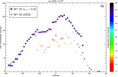
2019). Figure18shows the latitudinal profile of H2O at the time

of the TEXES observations (MY 34, Ls = 205–215◦_{), as derived}

from PFS observations. It can be seen that the H2O column

den-sity is depleted by a factor of almost 2 with respect to MY 29, a Martian year corresponding to a low dust content. This seems to imply that the dust content during the MY 34 global dust storm

H2O No dust H2O2 No dust

H2O Dust H2O2 Dust

ppmv ppbv ppmv ppbv Al (tu de (k m ) Al (tu de (k m ) Al (tu de (k m ) Al (tu de (k m )

Solar longitude Solar longitude

Fig. 17. Vertical distributions of H2O (left) and H2O2 (right) as a

function of the solar longitude at the beginning of southern summer (Ls = 180–220◦_{) Top: clear conditions; bottom: dusty conditions.} Sim-ulations were done with the GEM model (Daerden et al. 2019) for the latitude of the subsolar point (12◦_S).

Fig. 18. Latitudinal variations in the water vapor column density

observed by PFS berween Ls = 205◦ _{and 215}◦ _{in the case of MY 29,} corresponding to a dust opacity lower than 0.4 (stars), and M34, a great dust storm (crosses). The color bar on the right of the figure indi-cates the integrated dust opacity. The figure is taken fromGiuranna &

Wolkenberg(2019).

was actually higher than assumed in the simulations shown in

Figs. 14 and 15. A factor 2 decrease of H2O column density

might have led to a similar depletion of the H2O2column density.

The decrease of water vapor at middle latitudes is thus a

plau-sible explanation for the low upper limit of H2O2 inferred by

TEXES.

The depletion of water vapor in the Martian atmosphere in the presence of a high dust content is being studied in detail by Giuranna & Wolkenberg (2019). This paper, based on the PFS database, shows that H2O was strongly depleted during the MY 28 and MY 34 global dust storms. As a possible explana-tion, the authors suggest that the water vapor depletion could be due to the shading of the surface by the optically thick dust and the subsequent cooling of the surface, which would lead to water adsorption by the regolith, acting as a relative sink for water

dur-ing the course of the dust storm (Boettger et al. 2004,2005).

Another possible explanation, proposed byFouchet et al.(2011),

is the nearly isothermal profile that would prevent convection from the boundary layer to the general convection cell.

(11)

4.3. Seasonal behavior of H₂O₂

As shown in Fig.15, the recalibration of the H2O2dataset has an

important impact on our understanding of the seasonal behavior

of H2O2. First, the general overall agreement mentioned in

ear-lier publications is significantly degraded. Second, we can see

on four occasions (Ls = 77, 112, 150, and 209◦_{) that there is a}

contradiction between the H2O2 measurements recorded at the

same season during different Martian years. We showed that the presence of the MY 34 global dust storm can explain the

low value of H2O2 in July 2018 (Ls = 109◦_{). However, three}

other cases remain unexplained. Two of them occur near aphe-lion, and the third occurs before the autumn equinox. The good

agreement observed between the H2O2observation of May 2016

(Ls = 148.5◦_{) and the models could indicate that, while the}

nor-mal seasonal behavior of H2O2 is accurately described by the

models, another factor of unknown origin occasionally inhibits

the H2O2production.

A final remark has to be made about the need to use heteroge-neous chemistry to account for the seasonal variations in H2O2.

It was pointed out in our previous studies that the H2O2

mea-surements tended to support the heterogeneous model developed byLefèvre et al.(2008). However, Fig.15shows that the recent

GEM model developed byDaerden et al.(2019), which does not

include heterogeneous chemistry, is close to the heterogeneous

model of Lefèvre et al. (2008) in the seasons for which data

are available; it is also closer to the data than the LMD-MGCM

model for Ls around 150◦ _{and 200}◦_{. Further investigations are}

ongoing to better understand the differences between the two models. Our new measurement of May 2016, if we take into account the error bars, is in agreement with the two models; how-ever, it does not help us to discriminate between the gas phase and the heterogeneous photochemical models, as the two models are consistent within the error bars at that time of the season. 5. Conclusions

In this paper, we described two observations of H2O2 on Mars

obtained near the 2016 and 2018 oppositions, when the diameter of Mars was 17 and 23 arcsec, respectively. The May 2016

obser-vation was obtained near the southern equinox (Ls = 148.5◦_),

when the H2O2abundance is expected to be at its maximum. Our

result (45 ± 10 ppbv in the northern hemisphere) is in agreement

with the LMD-MGCM models ofLefèvre et al.(2008) and also,

more marginally, with the GEM model ofDaerden et al.(2019).

Our second observation (July 2018, Ls = 209◦_{) took place in the}

middle of the M34 global dust storm. In contrast with our first

observation of June 2003 (Ls = 206◦_{, H}₂_O₂_{= 18.2 ± 4.0 ppbv),}

we obtained a stringent 2σ upper limit of 10 ppbv. Based on PFS observations of the water vapor content at the same

time (Giuranna & Wolkenberg 2019), and GEM simulations by

Daerden et al.(2019), we propose that the H2O2depletion is due

to the depletion of water, which leads to the lack of HO2radicals.

Comparison between the recalibrated H2O2 dataset and

the different models suggests that overall the observed

abun-dance of H2O2 is lower than predicted, in turn suggesting

that the Martian atmosphere is less oxydizing than expected by photochemical models. It should also be noted that the

GEM model using gas-phase chemistry (Daerden et al. 2019)

and the LMD-MGCM model using heterogeneous chemistry (Lefèvre et al. 2008) are generally consistent, and both are above

the observed seasonal variations in H2O2. As a consequence, our earlier conclusion about the indication of heterogeneous

chemistry in the photochemical cycle of H2O2 may have to

be revisited. Finally, the evidence for inter-annual variabilities

of H2O2 requires further investigations using photochemical

models. In the future, measurements should concentrate on the

season around the autumn equinox (Ls = 150–230◦_{), when the}

difference between the two models is greatest.

Acknowledgements.T.E. and T.K.G. were visiting astronomers at the Infrared Telescope Facility, which is operated by the University of Hawaii under coop-erative agreement no. NNX-08AE38A with the national Aeronautics and Space Administration, Science Mission Doctorate, Planetary Astronomy Program. We wish to thank the IRTF staff for the support of the TEXES observations. T.K.G. acknowledges the support of NASA Grant NNX14AG34G. T.E. and B.B. acknowledge support from CNRS and the Programme National de Planétologie.

References

Aoki, S., Richter, M., DeWitt, C., et al. 2018,A&A, 610, A78

Atreya, S. K., & Gu, Z. G. 1995,Adv. Space Res., 16, 57

Boettger, H. M., Lewis, S. R., Read, P. L., & Forget, F. 2004,Geophys. Res. Lett., 31, L22702

Boettger, H. M., Lewis, S. R., Read, P. L., & Forget, F. 2005,Icarus, 177, 174

Camy-Peyret, C., Flaud, J.-M., Johns, J. W. C., & Noel, M. 1992,J. Mol. Spectr., 155, 84

Clancy, R. T., & Nair, H. 1996,J. Geophys. Res., 101, 12785

Clancy, R. T., Sandor, B. J., & Moriarty-Schieven, G. H. 2004,Icarus, 168, 116

Daerden, F., Neary, L., Viscardy, S., et al. 2019,Icarus, 326, 197

Encrenaz, T., Bézard, B., Greathouse, T. K., et al. 2004,Icarus, 170, 424

Encrenaz, T., Greathouse, T., Bézard, B., et al. 2010,A&A, 520, A33

Encrenaz, T., Greathouse, T. K., Lefèvre, F., et al. 2012,Planet. Space Sci., 68, 3

Encrenaz, T., Greathouse, T., Lefèvre, F., et al. 2015,A&A, 528, A127

Fedorova, A., Bertaux, J.-L., Betsis, D., et al. 2018,Icarus, 300, 440

Flaud, J.-M., Camy-Peyret, C., John, J. W. C., & Carli, B. 1989,J. Chem. Phys., 91, 1504

Forget, F., Hourdin, F., Fournier, R., et al. 1999,J. Geophys. Res., 104, 24155

Fouchet, T., Moreno, R., Lellouch, E., et al. 2011, Planet. Space Sci., 59, 683

Giuranna, M., & Wolkenberg, P. 2019, Icarus, submitted

Jacquinet-Husson, N., Arié, E., Ballard, J., et al. 1999,J. Quant. Spectr. Rad. Transf., 62, 205

Jacquinet-Husson, N., Scott, N. A., Chédin, A., et al. 2005,J. Quant. Spectr. Rad. Transf., 95, 429

Jacquinet-Husson, N., Scott, N. A., Chédin, A., et al. 2008,J. Quant. Spectr. Rad. Transf., 109, 1043

Jacquinet-Husson, N., Crepeau, L., Armante, R., et al. 2011,J. Quant. Spectr. Rad. Transf., 112, 2395

Jacquinet-Husson, N., Armante, R., Scott, N. A., et al. 2016,J. Mol. Spectr., 327, 31

Kass, D. M., Kleinboehl, A., Shirley, J. H., et al. 2018, Communication presented at the AGU Fall Meeting, 10–14 Dec. 2018, Washington DC, USA

Klee, S., Winnewisser, M., Perrin, A., & Flaud, J.-M. 1999,J. Mol. Spectr., 195, 154

Krasnopolsky, V. A. 1993,Icarus, 101, 313

Lacy, J. H., Richter, M. J., Greathouse, T. K., et al. 2002,PASP, 114, 153

Lefèvre, F., Bertaux, J.-L., Clancy, R. T., et al. 2008,Nature, 454, 971

Montmessin, F., Korablev, O., Lefèvre, F., et al. 2017,Icarus, 297, 195

Moudden, Y. 2007,Planet. Space Sci., 55, 2137

Oyama, V. I., & Berdahl, B. J. 1977,J. Geophys. Res., 82, 4669

Perrin, A., Valentin, L., Flaud, J.-M., et al. 1995,J. Mol. Spectr., 171, 358

Perrin, A., Flaud, J.-M., Camy-Peyret, C., et al. 1996,J. Mol. Spectr., 176, 287

Pollack, J. B., Dalton, J. B., Grinspoon, D., et al. 1993,Icarus, 103, 1

Smith, M. D. 2004,Icarus, 167, 148

Smith, M., Daerden, F., Neary, L., & Khayat, A. 2018,Icarus, 301, 117

Trokhimovskiy, A., Fedorova, A., Korablev, O., et al. 2015,Icarus, 251, 50

Vandaele, A. C., Betsis D., Ivanov Y. S., et al. 2019,Nature, 568, 521