* Development and Inflight Validation
of an Automated Flight Planning System
Using Multiple-Sensor Windfield Estimation
by
Andrew Kevin Barrows S.B., Aeronautics and Astronautics Massachusetts Institute of Technology, 1989
Submitted to the Department of Aeronautics and Astronautics in Partial Fulfillment of the Requirements for the Degree of
MASTER OF SCIENCE in Aeronautics and Astronautics
at the
MASSACHUSETTS INSTITUTE OF TECHNOLOGY June 1993
@ Massachusetts Institute of Technology 1993
All rights reserved
Signature of Author
Department of Aeronautics and Astronautics May 7, 1993
Certified by
Accepted by
Associate Professor R. John Hansman Department of Aeronautics and Astronautics Thesis Supervisor
SVrofessor Harold Y. Wachman Chairman, Department Graduate Committee
MASSACHUSETTS INSTITUTE
OF TFCN OPY
Development and Inflight Validation
of an Automated Flight Planning System
Using Multiple-Sensor Windfield Estimation
by
Andrew Kevin Barrows
Submitted to the Department of Aeronautics and Astronautics on May 7, 1993 in partial fulfillment of the requirements for the Degree of
Master of Science in Aeronautics and Astronautics
Abstract
Automated flight planning algorithms have been developed for aircrew decision aiding and primary mission control of autonomous air vehicles. Capabilities include
multiple levels of strategic and tactical planning. These algorithms are typically evaluated in simulations where sensor performance and component integration are assumed to be ideal. In a practical system however, sensor fusion and component integration are likely to be performance- and cost-limiting factors. This project addressed fundamental integration issues through implementation of a multiple-level planning system on a microcomputer interfaced to various sensors, and flight testing onboard a single-engine general aviation aircraft.
Strategic flight plans were generated using a directed nodal search technique. Planning consisted of the minimum-time altitude profile over a great-circle route between two points, with the winds as the primary external influencing factor. Improvements made over existing trajectory planning algorithms included 1) introduction of virtual nodes at top-of-climb and top-of-descent points to allow highly accurate predictions of time enroute, and 2) addition of a time penalty on climb and descent legs to reflect the real costs associated with transitions in flight condition. Planning was based on a world model that included representations of winds and temperatures aloft, aircraft performance, ground facilities, and terrain. The wind and temperature model allowed real-time fusion of multiple-sensor data with forecast information to arrive at an improved estimate of atmospheric conditions. Flights made with intentionally-flawed initial wind forecasts showed that the system could quickly learn (through in-situ measurements) and adapt flight plans to actual conditions. Tactical planning algorithms that responded to a real or simulated collision hazard or engine failure were also successfully flight tested. After the tactical deviations, the system
evaluated options to reacquire the original strategic plan or generate a new one. Flight testing indicated that, by increasing the computational power available, the planning system
architecture is fundamentally adaptable to more complex flight planning problems.
Probabilistic planning methods were introduced as a means of dealing with uncertainties in measurements and in the world model.
Thesis Supervisor: Dr. R. John Hansman
Acknowledgments
My deepest gratitude goes to my mother Nancy and sister Kristen for their love and
support. The high value placed on education by my family -including my father -is what really made this thesis happen.
Prof. John Hansman was my teacher, mentor, sounding board, and flight test pilot throughout this research. His insights, constructive criticism, and sound advice always challenged me to provide focus and direction to this project. Thanks for making me a better thinker, researcher, and writer!
I am indebted to Victor, Keiko, Paula, Jim, Adam, Ed, Alan, JP, Myk, Craig, Lee, Mark, Marc, and Amy, the graduate students of the M.I.T. Aeronautical Systems
Laboratory, for a seemingly-endless stream of distractions and stimulating conversations. The late-night lab sessions will be remembered as some of the best times from graduate school! The efforts of the following students who assisted the project through M.I.T.'s Undergraduate Research Opportunities Program are also sincerely appreciated: Marc Amar, Andrew Belinky, Richard Brawn, Amy Gardner, Edward Hahn, Erik Larson, Trudy Liu, Andrew McFarland, Jeffrey Olson, and Oliver Sostre. Paul Bauer provided invaluable assistance as a flight test pilot and expert advisor on design of the flight test electronics.
Special thanks to John Araki, Sally Araki, T.J. Cradick, Ben DeSousa, Jack Kotovsky, Don Woodlock, the Necky Kayak Company, Korg Musical Instruments, Yamaha Musical Instruments, Aero Eagles Soccer, Nice Bumps Volleyball, 'Da Nasty and Bedside Prophets, Cessna Aircraft, Gary Fisher Mountain Bikes, Bridgestone Mountain Bikes, Spectrum HoloByte Software (makers of TETRISm), Prof. Ed Crawley and the
staff and students of Unified Engineering 1991-92, and Gus. Without them, this thesis would have been finished much, much sooner.
This research was supported by the Charles Stark Draper Laboratory under its Independent Research and Development Program.
Contents
A bstract ... 2 Acknowledgments ... 3 Contents...4 List of Figures ... 8 List of Tables ... 10 Nomenclature... 11 1 Introduction ... 131.1 Automated Flight Planning Systems... ... 13
1.2 Previous Research ... ...14
1.3 Problem Statement and Objective ... 15
1.4 Planning Algorithms... ... 16 1.4.1 Strategic Planning ... ... 16 1.4.2 Tactical Planning...18 1.5 Sensor Fusion ... 18 1.6 Mission Management ... ... 20 1.7 Overview ... ... 20 2 Planning Algorithms ... 22 2.1 Trajectory Planner... 22 2.2 Search Method ... 22
2.2.1 Directed Search Methods... 22
2.2.2 Uniform-Cost Search...23
2.3 Node Network ... 24
2.4 Aircraft Performance Model ... ... ... 25
2.5 Cost Function... 26
2.6 Distinguishing Features of The Flight Planning Problem ... 26
2.6.1 Variance of Connectivity With State ... 26
2.6.2 Variance of Cost Function With State .... ... ... 27
2.6.3 Breakdown of Climb and Descent Arcs ... 28
2.6.4 Altitude Transition Penalty... . ... 28
2.7 Probabilistic Planning ... .. 29
2.8 Collision Avoidance Planner... ... 31
2.9 Engine-Out Planner ... ... 31
3 W orld M odel... 32
3.1 Wind and Temperature Model ... ... 32
3.1.1 Weighted Averaging Scheme... ... 33
3.1.2 Horizontal Weighting ... 34
3.1.3 Altitude Weighting ... 34
3.1.4 Time Weighting ... ...35
3.1.5 Measurement Weighting ... ... ... 35
3.2 Magnetic Variation Model ... 36
3.3 Terrain Model... ... 37
4 Flight Test Hardware ... 38
4.1 Test Aircraft ... 38
4.2 Flight Hardware... ... 38
4.2.1 Instrumented Pallet ... ... 39
4.2.2 Computer ... 41
4.2.3 Position Sensing ... 42
4.2.5 Directional Gyroscope ... 44
4.2.6 Sampling Procedure ... 44
4.3 Wind and Temperature Measurements ... 44
5 Strategic Planning Tests...46
5.1 Procedure ... 46
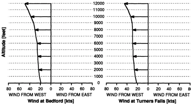
5.2 Winds Aloft Forecasts ... 47
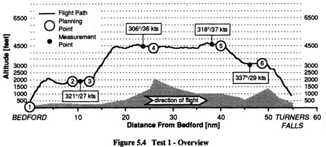
5.3 Test 1: Bedford to Turners Falls -Good Wind Forecast ... 49
5.4 Test 2: Turners Falls to Bedford -Good Wind Forecast ... ...54
5.5 Test 3: Bedford to Turners Falls -Bad Wind Forecast...57
5.6 Test 4: Turners Falls to Bedford -Bad Wind Forecast ... 62
5.7 Discussion ... 65
5.7.1 Strategic Planner Performance ... ... 65
5.7.2 Wind Measurement Errors... ... 65
5.7.3 Air Data Acquisition ... ...67
6 Tactical Planning Tests ... ... 69
6.1 Collision Avoidance Planner Test...69
6.1.1 Procedure ... 69
6.1.2 Discussion... 71
6.2 Engine-Out Planner Test ... ... ... ... 71
6.2.1 Procedure ... 71 6.2.2 Discussion ... 73 7 Conclusion ... 74 7.1 Strategic Planning... ... 74 7.2 Tactical Planning ... ...75 7.3 Sensor Fusion ... 76
7.4 Probabilistic Planning ... ... ... ... 76
7.5 Summary ... .. 77
References ... ... 78
Appendix A -Uniform-Cost Search ... 80
Appendix B -Performance Curves ... 82
Appendix C -Probabilistic Wind Model ... 84
C . 1 Introduction ... 84
C.2 Wind Forecast Representations...84
C.3 The Atmosphere as a Random Process ... 85
C.4 The Forecast Vector... ... 88
C.5 Measurement Integration ... 89
C.6 Application Examples... 92
C.6.1 Top of Climb Point Prediction ... ...92
C.6.2 ETA Prediction ... 96
C.7 Limitations ... 97
C.8 Sampling Rate Considerations...98
List of Figures
Figure 1.1 Figure 1.2 Figure 1.3 Figure 1.4 Figure 2.1 Figure 2.2 Figure 2.3 Figure 3.1 Figure 4.1 Figure 4.2 Figure 4.3 Figure 4.4 Figure 5.1 Figure 5.2 Figure 5.3 Figure 5.4 Figure 5.5 Figure 5.6 Figure 5.7 Figure 5.8 Figure 5.9 Figure 5.10 Figure 5.11 Figure 5.12 Figure 5.13 Figure 5.14 Figure 5.15 Figure 5.16 Figure 5.17 Figure 5.18 Figure 5.19 Figure 5.20 Figure 5.21 Figure 5.22Automated Planning System Integration ... 13
Planning System Structure...16
Flight Planning Problem ... 17
Fusion of Sensor Data...19
Node Connectivity -Node B Reachable From Node A ... 27
Node Connectivity -Node B Unreachable From Node A ... 27
Breakdown of Climb Leg From Node A to Node B...28
Time Weighting Function ... ...36
Piper Arrow IV Test Aircraft ... 39
Instrumentation Schematic...40
Instrumentation Pallet ... 41
S-NAV Air Data Sensing Computer ... 43
Flight Test Region ... 46
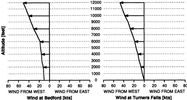
"Good" Wind Forecast Profile used for Trajectory Planner Tests...48
"Bad" Wind Forecast Profile used for Trajectory Planner Tests ... 49
Test 1 -Overview... ... ... 50
Test 1 -"Good" Initial Wind Forecast Profile ... 50
Test 1 -Estimated Wind Profile After Three Measurements ... 51
Test 1 - Flight Plan 1 ... 52
Test 1 - Flight Plan 2 ... 52
Test 1 - Flight Plan 3 ... ...52
Test 1 - Flight Plan 4 ... ... ... ... 53
Test 1 - Flight Plan 5 ... ... 53
Test 1 - Flight Plan 6 ... 53
Test 2 - Overview ... .. 54
Test 2 - Estimated Wind Profile After Four Measurements ... ...55
Test 2 - Flight Plan 1 ... 55
Test 2 - Flight Plan 2 ... 56
Test 2 - Flight Plan 3 ... 56
Test 2 - Flight Plan 4 ... ... 56
Test 3 -Overview...57
Test 3 -"Bad" Initial Wind Forecast Profile...58
Test 3 - Estimated Wind Profile After One Measurement ... ...58
Figure 5.23 Test 3 - Estimated Wind Profile After Three Measurements ... 59
Figure 5.24 Test 3 - Estimated Wind Profile After Four Measurements ... 60
Figure 5.25 Test 3 - Estimated Wind Profile After Five Measurements ... 60
Figure 5.26 Test 3 -Flight Plan 1 ... 61
Figure 5.27 Test 3 - Flight Plan 2 ... ... 61
Figure 5.28 Test 3 -Flight Plan 5 ... ... 62
Figure 5.29 Test 4 - Overview ... 62
Figure 5.30 Test 4 - Estimated Wind Profile After Three Measurements ... 63
Figure 5.31 Test 4 - Flight Plan 1 ... 64
Figure 5.32 Test 4 - Flight Plan 2 ... 64
Figure 5.33 Test 4 - Flight Plan 4 ... ... 64
Figure 5.34 Test 1 -Estimated Wind Profile After Three Measurements... ... 66
Figure 5.35 Test 2 - Estimated Wind Profile After Four Measurements ... 67
Figure 6.1 Wind Forecast used for Collision Avoidance Planner Test... 70
Figure 6.2 Collision Avoidance Planner Test... ... 70
Figure 6.3 Engine-Out Planner Test ... 72
Figure 6.4 Map View of Engine-Out Planner Test...73
Figure B.1 Fuel, Time, and Distance to Climb ... 82
Figure B.2 Speed Power Performance Cruise ... 83
Figure B.3 Fuel, Time, and Distance to Descend...83
List of
Table 2.1 Table 5.1 Table 5.2 Table 5.3 Table C.1Tables
Node Altitudes ... 25Trajectory Planner Flight Test Matrix ... 47
Winds Aloft Forecast at Boston, Massachusetts ... 47
Winds Aloft Forecast at Albany, New York...48
Nomenclature
The meanings of variables and symbols used in this work are summarized here, with the chapters where they are used shown in parentheses.
A segment time tailwind coupling matrix (Appendix C)
b segment time constant vector (Appendix C)
C wind measurement matrix (Appendix C)
dTIC distance to top of climb point (Appendix C)
d vector of segment distances (Appendix C)
E segment tailwind extraction matrix (Appendix C)
ETA vector of waypoint estimated arrival times (Appendix C)
f(n) cheapest cost from start node through node n to goal node (2)
g(n) cost from start node to node n (2)
G S groundspeed vector (3, Appendix C)
h(n) heuristic function at node n (2)
K Kalman gain matrix (Appendix C)
L lower triangular matrix (Appendix C)
mi measurement/forecast flag for i-th meteorological datapoint (3)
n' successor of node n (2)
Rij (i, j) element of wind correlation matrix (Appendix C) r reference point for wind and temperature retrieval (3)
ri location of i-th meteorological datapoint (3)
ROC vector of segment climb rates (Appendix C)
s start node (2)
ST vector of segment thicknesses (Appendix C)
t reference time for wind and temperature retrieval (3)
ti time when i-th meteorological datapoint was generated (3)
t vector of segment times (Appendix C)
TAS true airspeed vector (3, Appendix C)
ui V vi wi Whi Wmi Wti Wvi W x-x+ z
Oij
0 e av X(TW) I E-C+i-th component of wind fluctuation vector (Appendix C) scalar variable retrieved from meteorological model (3) value of v at i-th meteorological datapoint (3)
weighting of i-th meteorological datapoint (3)
horizontal weighting of i-th meteorological datapoint (3) measurement weighting of i-th meteorological datapoint (3) time weighting of i-th meteorological datapoint (3)
vertical weighting of i-th meteorological datapoint (3) wind vector (3)
wind forecast vector (Appendix C)
a priori mean wind forecast vector (Appendix C) a posteriori mean wind forecast vector (Appendix C) vector of wind measurements (Appendix C)
(i, j) element of wind power spectral density matrix (Appendix C) white noise vector (Appendix C)
white noise covariance matrix (Appendix C) horizontal weighting shape factor (3) altitude weighting shape factor (3)
covariance matrix of segment tailwinds (Appendix C) wind forecast covariance matrix (Appendix C)
a priori wind forecast covariance matrix (Appendix C) a posteriori wind forecast covariance matrix (Appendix C) time displacement (Appendix C)
spatial displacement vector (Appendix C) time frequency (Appendix C)
1 Introduction
1.1 Automated Flight Planning Systems
Flight planning algorithms have been developed for generating dynamic mission plans that govern flight routing and resource allocation. These algorithms can be used as decision aids by flight crews or function as the mission controller on an autonomous air vehicle. Planning may be done at the strategic level (e.g. generating minimum-fuel or minimum-time flight trajectories) or tactically, in response to unpredicted situations (e.g. a loss of power or another aircraft posing a collision hazard).
These systems base plans on dynamic world models of the factors that affect a flight. Wind, storm activity, turbulence, icing, positions of nearby aircraft, and many other factors evolve in ways that are not fully known or determined before the flight begins. Models rely on a combination of forecast information and direct measurements
Varying Conditions
Mission
Requirements t -6 %6 % f Guidance Flight
and Constraints ig
AtaePann m Path
PLANNING 1.1 atot PILOT OR y VEHICLE
> ALGORITHMS AUTOPILOT ESTIMATE OF Sensor CURRENTAND Fusion " - SENSORS FUTURE SCONDITIONS
SAutomated Planning System
of these variables to accurately reflect actual conditions. Sensor fusion consists of integrating measurements into prior estimates to intelligently update these models. Planning algorithms are then used to generate guidance commands based on these
models. If mission planning can be thought of as the outermost guidance loop in aircraft flight, then planning algorithms with fused sensor information "close the outer guidance loop," as illustrated in Figure 1.1.
1.2 Previous Research
Much work has been done on developing algorithms designed to aid in flight planning and resource allocation. Simple route optimizations were being performed on
ground-based computers in the mid 1960s [Rose, Simpson et al.]. More recently, studies of integrated decision-aiding systems [Corrigan and Keller, Glickstein], and pilot-vehicle interface issues [Layton et al.] have been conducted.
The role of automated flight planning algorithms for autonomous air vehicles (AAVs) has received much attention [Adams and Hansman]. Planning algorithms will perform flight routing and high-level mission control for AAVs, either alone or in
coordinated squadrons. Current unmanned air vehicle systems typically require a human operator during some portion of flight (e.g. landing) and follow an "open-loop"
preprogrammed set of commands for routing and resource allocation.
Military applications studied have included reconnaissance, target selection and ordering, route planning, and munitions use. Additional factors taken into account typically include exposure to threats such as surface-to-air missile sites, effectiveness in destroying a target, terrain radar masking, radar cross section exposure, and a host of others.
1.3 Problem Statement and Objective
Research on automated planning systems has relied heavily on laboratory simulations where sensor performance and component integration are assumed to be ideal. In a practical planning system however, issues such as sensor fusion and component integration are likely to be performance-limiting or cost-limiting factors. However, the difficulty and high cost of flight testing has limited the amount of work done in this area. This experimental effort addressed the need for flight testing of operational planning systems. The goal of this project was to identify fundamental
system integration issues through implementation of a flight planning system using real-time sensor measurements on an actual vehicle.
Automated planning software, flight-ready computer and sensor hardware, and a flight test program were developed for this investigation. Flight testing was done on a
single-engine light aircraft under visual flight rules (VFR) in the New England region. Tests dealt with planning of a straight-line trajectory between two points, yielding a two-dimensional problem (distance along a line and altitude) with the wind being the primary environmental factor that influenced the problem. The ability of the system to react to unexpected situations was also investigated by implementing algorithms that could generate tactical responses to traffic hazard and power loss situations. These simplified problems retained the important features of more general problems (unpredictable events
and imperfect knowledge of aircraft performance and environmental conditions), permitting identification of sensor fusion and system integration issues without
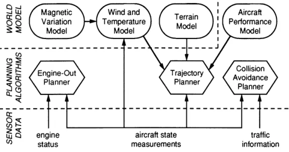
unnecessary complications. The structure of the automated planning system is shown in Figure 1.2.
The planning algorithms accepted sensor data, propulsion status, and traffic status as inputs along with user commands to generate textual guidance commands for the pilot. Wind measurements (made by comparing airspeed and groundspeed vectors) were
J Magnetic Wind and I Aircraft
cc Q Terrain
E Engine-Out Trajectory
z c Planner Planner oane
S engine aircraft state traffic
(I status measurements information
Figure 1.2 Planning System Structure
taken periodically and then fused into the wind and temperature model. Models of terrain and magnetic variation were also used by the planning algorithms. These models taken together form the world model on which the planning algorithms operated. A
performance model of the test aircraft was also employed by the planning system.
1.4 Planning Algorithms
Planning systems typically employ a hierarchical structure separating the planning problem into global and more detailed components that represent multiple levels in the planning process. These sub-tasks tend to fall within a spectrum of planning processes that range from strategic to tactical in nature.
1.4.1 Strategic Planning
Strategic planning affects long-range optimality of the flight in a global manner. For a mission with multiple stops or targets, selection and ordering of objectives
constitutes part of the strategic planning process. Strategic planning also includes generation of flight trajectories defined as sets of waypoints and/or schedules of airspeeds, climb rates, control inputs, etc.
For this project, a strategic trajectory planner was implemented that found the minimum-time path between two points. The winds aloft and aircraft performance were
the primary factors affecting the optimum strategic plan. The planning algorithm was based on techniques derived from directed search methods. These methods typically operate on a network of "nodes" that represent different stages in solving a problem. Such techniques search the paths leading from the starting node to the "goal" node, with the ultimate objective of finding the path which minimizes a specified cost function. The nodal network for the flight planning problem, depicted in Figure 1.3, filled the airspace between the starting point and the destination airport. The cost function optimized was a linear combination of the total fuel burn and trip duration. In addition to this cost
function, a "hard" constraint was imposed on fuel burn since it is limited by the maximum fuel load of the airplane.
Altitude Flight Path Profile of Winds Aloft
i
2,000' 10,000'0 0 0 0 * * * * 0 8,000'e * 0 0 0 0 0 6,000'4 * * 4 * 0 * 4,000'4 * * - - * * 2,000' 4A D ADeparture Airport Destination Airport
0 NM 40 NM 80 NM 120 NM 160 NM
Distance From Departure Airport
1.4.2 Tactical Planning
Tactical planning includes short-term procedures necessary to deal with unexpected, unpredicted, or emergency situations. Situations which require tactical planning tend to last for only a fraction of the flight duration, but may have implications for the remainder of the flight. Examples include deviations around thunderstorms and altitude transitions to escape turbulence and icing. Autonomous aircraft will need the capability to generate plans to escape populated areas in the event of an equipment failure. This has been identified as critical to the acceptance of AAVs for civilian applications [Adams and Hansman].
This project investigated performance of a tactical planner to generate maneuvers to avoid nearby traffic. When a real or simulated traffic encounter ended, the pilot could recapture the original strategic flight plan or -if the tactical maneuver left the aircraft
significantly off the original plan -a new strategic plan could be generated. A second tactical planner was implemented to provide guidance to a suitable airport after a
simulated engine failure in the single-engine test aircraft.
1.5 Sensor Fusion
The modeled environmental variables which influence a flight range from constantly changing factors, such as the windfield, to factors which are essentially constant, such as terrain and ground facilities (i.e. airport locations and runway
information). Accuracy of these static and dynamic world models is key to the success of a planning system; optimized trajectories are only as good as the assumptions on which they are based.
The winds aloft have a fundamental effect on the desirability of one flight altitude over another. The optimum routing and altitude profile is a complex balance between aircraft performance, the windfield, terrain features, and the length of the flight. Since
the windfield constantly changes on time scales comparable to or shorter than a typical flight, it is necessary to use a dynamic representation capable of representing variations of these quantities.
While forecasts of these changing variables are readily available, the well-documented decrease in accuracy over time of winds aloft forecasts [Hollister et al.] dictates that current wind measurements are a necessary supplement to forecast values for flight planning. Forecast information still has great value, however, especially for points and times near which no measurements are available. Both types of information clearly have their place in a complete atmospheric description, so that a scheme such as the one outlined in Figure 1.4 is needed for intelligently fusing sensor measurements into an existing forecast to arrive at an updated estimate of present and future conditions.
estimate of
current wind and temperature measurement present and
future
(one datapoint) conditions
SENSOR FUSION
estimate of present and future conditions (many datapoints)
Figure 1.4 Fusion of Sensor Data
An aircraft using advanced flight planning algorithms can make periodic wind and temperature measurements to improve its meteorological model, or even use data
obtained from external sources such as balloon soundings and wind profilers. The technology now exists to send aircraft-based measurements via datalink [Benjamin et al.] to a ground facility or other aircraft where multiple measurements can be fused with a forecast to form a current estimate of meteorological conditions. The success of a planning system's dynamic wind model, and hence of the planning system as a whole, is limited by methods used for sensor fusion.
The flight test system's dynamic wind and temperature model used a weighted averaging scheme to fuse inflight measurements into existing estimates of these variables. This method applied a weighting to each datapoint according to its distance (in time and space) from the point and time where wind and temperature were to be estimated. Nearby datapoints had a strong influence on wind and temperature estimates, while distant datapoints carried very little weight.
1.6 Mission Management
The highest level of decision making, the mission management level, coordinates the multiple levels of strategic and tactical planning. The mission management role includes monitoring of the current flight plan to determine if it is satisfactory or, if it is not, initiating the strategic replanning process. When an unexpected condition requires a short-term change to the flight plan, the mission manager initiates creation of a tactical deviation from the planned trajectory. After a tactical maneuver, it determines whether to reacquire the original strategic plan or to generate a new one. During flight tests, the test engineer and pilot performed the mission management function by using lower-level strategic and tactical planners as decision aids. AAV applications will require dedicated mission management algorithms.
1.7 Overview
Details on the planning algorithms and world model elements used in flight testing are given in Chapters 2 and 3. Chapter 4 describes the novel, inexpensive approach used for flight testing including the test aircraft, computer, and sensing
hardware. Chapters 5 and 6 present and discuss data from flight testing of strategic and tactical planning algorithms. Conclusions of this work are presented in Chapter 7.
Appendix A is an algorithmic description of the uniform-cost search method used by the trajectory planner, and Appendix B contains performance curves used by the
aircraft performance model. A probabilistic wind model and application examples are presented in Appendix C.
2 Planning Algorithms
This chapter details the strategic trajectory planner and the aircraft performance model used to calculate flight plan costs. Probabilistic planning methods are then
discussed. Finally, the tactical engine-out and collision avoidance planners are described.
2.1 Trajectory Planner
The strategic trajectory planner generated altitude profiles over the great-circle route between a starting point (this could be an airport or a point in the air) and the destination airport. Textual output to the pilot consisted of a set of waypoints, crossing
altitudes, and ETAs. The pilot flew the commanded altitude profile by initiating climbs and descents at appropriate points specified by the planner. The next five sections provide details on the trajectory planner.
2.2 Search Method
2.2.1 Directed Search Methods
The strategic trajectory planner used a directed search method to find the
minimum-cost path through the two-dimensional nodal network shown in Figure 1.3. By avoiding repetitive calculations, directed searches provide an efficient way for
systematically evaluating paths from the starting node to the destination node. Two such methods are described below.
2.2.2 Uniform-Cost Search
The directed search method used by the planner was the uniform-cost search, which is categorized in the literature under the more general family of best-first searches [Pearl, Nilsson]. Best-first searches operate by keeping track of the cheapest path cost
g(n) found thus far from the start node to each node n. A loop through the iterative
procedure consists of selecting the node with the lowest cost g(n) and then expanding it, by exploring arcs leading away from n to other nodes. When exploring these node-to-node arcs, the search considers nearby successor node-to-nodes on the level, climb, and descent paths leading away from n. The cost of traversing the arcs between node n and each
successor n' is calculated and then added to g(n) to find g(n') for each successor. The node with the lowest cost is then expanded to begin another loop. The process repeats as the search moves forward from the start node through the nodal network until the
destination node is reached. Pointers are used to keep track of the solution path, with successor nodes pointing back to their parent nodes. A step-by-step algorithmic description of the uniform-cost search is given in Appendix A.
As the size of the search network increases, the time required to perform a uniform-cost search increases rapidly. The uniform-cost search was adequate for simple flight planning problems, but solving problems more complicated than the one addressed
by this project will require a faster search algorithm.
2.2.3 A* Search
The uniform-cost search may be significantly sped up by the introduction of a carefully-selected heuristic function. This function h(n) is an "educated estimate" of the cost from node n to the goal node and is added to g(n):
to arrive atf(n), an estimate of the cost of the cheapest path from the start to the goal that
is constrained to go through node n. Using this new estimatef(n) as the node expansion
criterion in the uniform-cost search results in the A* (pronounced A-star) search. If h(n) is chosen to always give an optimistic (i.e. low) estimate of the cost from n to the goal, the search is guaranteed to find the minimum-cost solution path. Use of a well-chosen heuristic results in a directed search that avoids spending computational time exploring arcs that are not part of the optimum solution.
The A* search has been applied successfully to trajectory planning problems [Niiya, Corrigan and Keller] and was used as the framework for the flight planning algorithm. Since the planner was sufficiently fast for flight test purposes (maximum planning time of 40 seconds), the heuristic function was set to zero, resulting in a uniform-cost search.
2.3 Node Network
The trajectory planning problem was defined in two spatial dimensions: distance along a line and altitude. Nodes were distributed on a two-dimensional grid with 11 horizontal positions and 11 vertical levels. The horizontal positions were at the start position and destination airport, with the remaining nine points evenly distributed between the two endpoints. Node altitudes included the VFR cruising altitudes
appropriate to the direction of flight, and 500-foot levels at and below 3000 feet. Altitudes above 12500' were not included since they were above the practical altitude range of the test aircraft (see Table 2.1).
After the grid was constructed, nodes at the start and destination altitudes were patched into the grid at their respective positions. Finally, exclusion zones were imposed
to account for terrain. Any node fewer than 1000 feet above ground level was removed from the network to ensure that flights would not be planned hazardously close to the
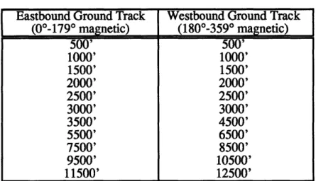
Table 2.1 Node Altitudes
Eastbound Ground Track Westbound Ground Track
(00-1790 magnetic) (1800-3590 magnetic) 500' 500' 1000' 1000' 1500' 1500' 2000' 2000' 2500' 2500' 3000' 3000' 3500' 4500' 5500' 6500' 7500' 8500' 9500' 10500' 11500' 12500'
ground. To allow departures and approaches at airports, nodes at and directly above the start and destination nodes were not removed.
2.4 Aircraft Performance Model
Arc costs were based on a performance model of the test aircraft. This model was represented as curve fits describing the following performance curves in the Arrow IV
Pilot's Operating Handbook [Piper Aircraft]:
FUEL, TIME, AND DISTANCE TO CLIMB
Associated Conditions: Power -2700 RPM, Full Throttle, Climb Speed - 90 KIAS
SPEED POWER PERFORMANCE CRUISE
Associated Conditions: Power -2400 RPM, 65% or Full Throttle above 9500' Density Altitude
FUEL, TIME, AND DISTANCE TO DESCEND
Associated Conditions: Power -2400 RPM, Throttle as Required, Descent Speed -146 KIAS
These curves are reproduced in Appendix B. The curves represented the standard climb, cruise, and descent flight conditions used throughout the flight test program. Although density altitude and aircraft weight were specified as inputs to the performance model, the curves were assumed to be insensitive to weight. This was a good assumption for light piston aircraft with their typically small (less than 0.2) fuel weight fractions.
Functional forms for the performance equations were verified in flight tests exploring several regimes of interest within the aircraft performance envelope.
Since performance characteristics remained effectively constant over the course of a single flight, a static performance model was used. In practice, aircraft performance changes over a period of years, usually due to deterioration in engine performance and condition of the aerodynamic surfaces. A quasi-static performance model can be gradually changed over the lifetime of the aircraft to reflect its varying performance. This can be done by performing periodic performance flight testing, or by a more
sophisticated scheme which continually updates a dynamic performance model during routine aircraft operation.
2.5 Cost Function
The cost function was implemented to allow any linear additive combination of trip duration and fuel burn. In practice, fuel burn was not weighted due to the difficulty
of obtaining accurate measurements of this variable for the test aircraft. Therefore, during flight tests the planner was configured to provide flight plans optimized for minimum time.
2.6 Distinguishing Features of The Flight Planning Problem
This section discusses several adaptations made to standard directed search techniques in order to reflect unique characteristics of the flight planning problem.
2.6.1 Variance of Connectivity With State
In most directed search applications, a node's successors can be determined before the search begins; one can tell which nodes are reachable from a given node before any costs are calculated. This was not the case with the flight planning problem considered here, since node connectivity varied with the states of the aircraft and
atmosphere. As an example, consider a climb arc between two nodes (Figure 2.1). Under certain wind conditions it might have been possible to accomplish this climb -node B was "reachable" from -node A.
* 0 B
0
WEAK TAILWIND
• A •
Figure 2.1 Node Connectivity -Node B Reachable From Node A
However, if there were a strong tailwind as in Figure 2.2, it may not have been possible to reach the final altitude before passing the position of node B (the aircraft would have been blown under node B). In order to retrieve the correct value of the
STRONG TAILWIND
SA A
*
Figure 2.2 Node Connectivity - Node B Unreachable From Node A
time-varying wind from the wind model, it was necessary to know when the aircraft would be flying along a given arc. Therefore, the estimated time was stored at each node
by the search algorithm to allow real-time determination of node connectivity.
2.6.2 Variance of Cost Function With State
Arc costs, in addition to node connectivity, were dependent on the state of the aircraft and atmosphere. The primary state variable affecting the time cost of a given arc was the headwind or tailwind component. The estimated time stored at each node was used to make real-time arc cost calculations based on winds when the arc was traversed.
2.6.3 Breakdown of Climb and Descent Arcs
Arcs involving climbs or descents were broken into two components: a climb or descent segment, and a level segment. An example climb arc is shown in Figure 2.3. Without this breakdown scheme, the planner would have had to assume a climb profile (shown as a dashed line) at non-standard power, airspeed, and climb rate conditions. (These control inputs would have been chosen to ensure that the climb profile intersected node B.) However, since typical aircraft operations are based on standard flight
VIRTUAL NODE
level segment
-SB
Figure 2.3 Breakdown of Climb Leg From Node A to Node B
conditions, it was desirable for the planner to adhere to these practical constraints. To allow a standard climb profile (corresponding to the airspeed and power settings in the aircraft performance model), a virtual node was created at the point where the standard profile intersected the altitude of node B. Standard cruise airspeed and power settings were assumed on the level segment. Different wind values were retrieved from the wind model for the two segments, allowing very accurate calculation of arc costs.
2.6.4 Altitude Transition Penalty
It was observed during preliminary flight testing that certain wind profiles could lead to plans that contained alternating climbs and descents in rapid succession. For example, small variations in the windfield structure might have caused the optimum altitude to oscillate between two altitudes (e.g. 5500' and 7500'). This tended to occur
when the wind component along the direction of flight was relatively constant with altitude. In such circumstances the time differences associated with cruising at one altitude versus another were relatively small, so that minor horizontal windfield variations could cause the optimum flight altitude to oscillate.
There is no doubt that these plans were the minimum-time profiles consistent with the estimated windfield and the specified cost function. However, there are inefficiencies associated with transitions in flight condition which were not modeled by the
performance curves used to describe the aircraft. For example, when the aircraft was transitioned between climb, cruise, and descent conditions, there were periods of
acceleration and deceleration during which the aircraft was not at the optimum speed for the current condition. It was clear that these transitions represented a real cost which should be considered in planning. For manned missions, there are additional crew workload costs associated with transitions in flight condition. Therefore, an altitude
transition penalty was added to the cost function for node-to-node arcs which included a climb or descent. The value of 12 seconds was determined empirically by planning flights using a simulated wind profile that was nearly constant with altitude. The transition penalty time was increased from zero until the optimum plans no longer contained multiple climb/descent cycles. This altitude transition penalty worked well in practice; during flight testing, the planner did not generate profiles with repetitive climbs and descents.
2.7 Probabilistic Planning
The transition penalty was instituted to account for factors not captured by the aircraft performance model. The atmosphere is an even more complex system,
possessing many characteristics which cannot be modeled deterministically by existing tools. As with unmodeled performance features, uncertainties in the winds aloft have real effects on costs optimized by the planner. (These may be cost penalties or cost savings;
sometimes the conditions are more favorable than predicted.) The planning methods above make no attempt at dealing with this uncertainty. Instead, they plan
deterministically by assuming that the wind model is an exact description of present and future conditions.
Accounting for measurement and modeling uncertainty is expected to yield lower operational costs when averaged over the course of many flights. This approach requires planning and sensor fusion methods fundamentally different from those previously
mentioned. Instead of finding the single optimum path through a deterministic windfield, a probabilistic planner considers multiple plans and the probabilistic nature of their costs. For example, when choosing among several cruise altitudes, a probabilistic planner
calculates the probability density function (PDF) of the cost associated with each altitude. An expected-value criterion is then applied to choose the cruise altitude which yields the lowest average cost. These PDFs change during a given flight as measurements are
made, letting evidence build in favor of keeping or changing the current flight plan.
Probabilistic solution techniques typically break a problem into stages, just as the trajectory planner broke the flight into node-to-node arcs. At each stage of the problem, all possible environmental conditions (e.g. a PDF of windspeeds that might be
encountered) are considered along with all possible actions (e.g. fly level, initiate a climb, or initiate a descent) to arrive at a choice that minimizes the expected value of a cost function. A prospective flight plan is adopted when its mean cost falls below that of the current plan. A framework for probabilistic representations of planning problems is
offered by the field of decision analysis [Drake and Keeney].
Probabilistic planning also requires a probabilistic description of cost-influencing environmental factors and their interrelationships. For example, a probabilistic wind
model describes not only the wind components themselves, but also covariances between the winds at different locations and times. A probabilistic wind modeling technique was
developed and is presented in Appendix C. Implementation of such a model requires significant processing capability to handle the large data sets which describe the variances and covariances of atmospheric variables. Planning algorithms which deal with this uncertainty are also significantly more complex, requiring representation of many possible environmental conditions and choices at each stage of a flight. Due to limitations of the microcomputer used, the flight test program did not include probabilistic planning.
2.8 Collision Avoidance Planner
The collision avoidance planner generated tactical deviations in response to real or simulated warnings from a Traffic Collision Avoidance Device (TCAD) or Traffic Alert and Collision Avoidance System (TCAS). When this mode was invoked, strategic planning was suspended and the user was issued a traffic avoidance maneuver. For
simplicity, only climbing and descending maneuvers were commanded. When the collision threat had been resolved, the user could either reacquire the original flight plan
or replan a new flight profile.
2.9 Engine-Out Planner
The tactical engine-out planner could be used during actual or simulated power loss events to provide guidance to a nearby airport. Given aircraft position and altitude, the engine-out planner searched a database for airports within gliding distance. An airport was considered usable if the aircraft was predicted to be at 500 feet or higher over the field, ensuring that a suitable landing pattern could be set up as the airport was
approached. If there were multiple airports satisfying this criterion, the airport with the highest predicted altitude over the field was designated as the primary airport. Updated magnetic bearing and distance to the primary airport were given to the pilot every 10
3 World Model
The various elements of the world model used by the planning system are described here. The world model included representations of wind, temperature, magnetic variation, and terrain.
3.1 Wind and Temperature Model
The dynamic meteorological model represented wind and temperature as functions of latitude, longitude, altitude, and time. The model was initialized with forecast information and updated in flight with fused sensor measurements.
Representation of atmospheric field variables was made difficult by the fact that the available measurements and forecast datapoints were randomly distributed in space and time; datapoints tended not to fall onto a structured grid of times and locations. For instance, aircraft-based measurements were made at scattered locations and times along the flight path, and forecasts were specified at reporting stations that were not evenly spaced. A filtering scheme was therefore needed to estimate wind and temperature
between stations -or between times at which data was specified. Such a method is referred to as an objective analysis in the meteorological literature.
The wind and temperature model employed a weighted averaging scheme based on the Barnes objective analysis for mesoscale datafields [Barnes]. The model was initialized before each flight with forecast datapoints numerically generated by the National Weather Service. The forecast profile at a reporting station was received as a
"stack" of wind and temperature datapoints at various altitudes (3000', 6000', 9000', and 12000' were used in flight testing). These forecast datapoints were only valid over a specified interval of several hours, so a time series of datapoints was specified at every reporting station and altitude. Forecast information was also tagged with the time when the numerical model was actually run, allowing computation of the "age" of a forecast datapoint. Inflight measurements were incorporated as single datapoints with a specific horizontal position, altitude, and time of measurement. Individual forecast and measured datapoints were handled in the same way by the model; a forecast datapoint was averaged into a wind estimate just like an inflight measurement. However, the weighting functions for these two classes of data were different, reflecting their distinct properties.
3.1.1 Weighted Averaging Scheme
Wind and temperature were estimated as weighted averages of the n forecast and measured datapoints in the model. The west-to-east wind component, south-to-north wind component, and temperature were handled as separate scalar variables. The formula used to estimate scalar variable v at location r and time t (called the reference location and time) was:
n
Sviwi(ri- r, ti - t, mi)
v(r, t)= i= (3.1)
wi(ri - r, ti - t, mi)
i=l
where vi is the value of v at the i-th datapoint and wi is the weight given to the i-th datapoint. The weighting given to a datapoint was a multiplicative combination of the following weighting factors:
Wh: horizontal displacement of the datapoint location, ri, from the reference location
Wt: time difference between when the datapoint was generated, ti, and the reference time
Win: whether the datapoint was measured or forecast (indicated by mi)
Nearby datapoints (in space and time) generally had a strong influence on local wind and temperature estimates, while distant datapoints carried very little weight. The
components of w = WhWvWtWm are described below.
3.1.2 Horizontal Weighting
The horizontal weighting function, like that used in the Barnes objective analysis
[Barnes], was a Gaussian-shaped function of distance:
Wh= exp( - Ir 2 (3.2)
This weighting function drops off with distance at a rate determined by oh.
Excessively large values of
oh
resulted in overly smoothed estimates, while choosing ohtoo small produced detail near datapoints but yielded an excessive loss of structure between datapoints.
The value of oah for forecasts was chosen as 40 nm to give a horizontal weighting of approximately 0.5 midway between reporting stations, which have an average spacing of 80-120 nm in the New England flight test region.
For measurements, hm was set to 30 nm based on the expected 15 nm spacing between inflight wind measurement points. This lower value of oh gave measured datapoints smaller regions of influence than forecast datapoints.
3.1.3 Altitude Weighting
The altitude weighting, Wv, for measurements was a Gaussian function of altitude similar to the horizontal weighting in equation (3.2). The value of avm = 2500 feet was
determined empirically by comparing the results of using different values on typical wind profiles.
Since forecast datapoints were disseminated in "stacks," a linear interpolation scheme -as opposed to a smoothing method based on Gaussian weighting -was used for forecast datapoints in the vertical dimension. For example, if the reference was at 4000 feet, a forecast datapoint at 3000 feet was given a weight of Wv = 2/3, a datapoint at 6000 feet was given a 1/3 weighting, and datapoints at 9000 and 12000 feet were assigned Wv = 0. For reference altitudes below 3000 feet, values were linearly extrapolated based on forecast datapoints at 3000 and 6000 feet.
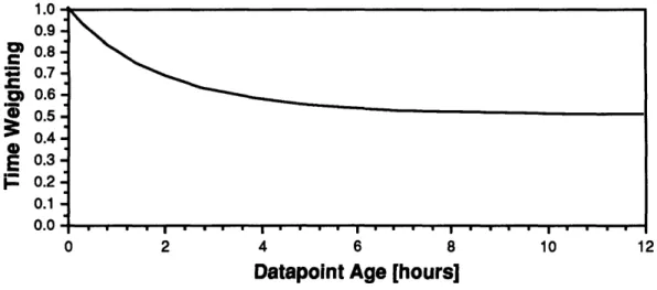
3.1.4 Time Weighting
As a datapoint grew older, its temporal weighting was decreased to reduce its influence on wind and temperature estimates. The "age" of a datapoint (whether
measured or forecast) was computed as the difference between the reference time and the time when the datapoint was generated, and then used as an argument to the time
weighting function, Wt. This function, shown in Figure 3.1, is an exponential decay from 1.0 to 0.5 with a time constant of 2 hours.
3.1.5 Measurement Weighting
Measurements provide a better description of the wind and temperature at a given point and time than do values estimated from forecast information. In regions near measurement points, it was essential that the model reflect measured values -not forecast values. An additional weighting factor, Wm, was therefore applied to measured
datapoints to influence wind and temperature estimates in favor of measurements. The weighting of Wm = 3.0 was determined empirically by comparing effects of various weightings on fusion of measurements into typical wind profiles. This value provided a
1.0 0.9 I 0.8 • 0.7 O 0.6 o.5 0.4
E
0.3S0.2
0.1 0.0 0 2 4 6 8 10 12Datapoint Age [hours]
Figure 3.1 Time Weighting Function
balance between the model not reflecting off-forecast conditions (if the measurement weighting was too small) and the model ignoring valuable forecast information (if the measurement weighting was too high)
Wm was simply set to 1.0 for forecast datapoints in order to produce the correct relative weighting between forecast and measured values.
3.2 Magnetic Variation Model
The world model also included a representation of magnetic variation used for fusion of wind direction measurements into the wind and temperature model. Wind measurements made in the aircraft were relative to magnetic north, because this was the format in which the navigational instruments output ground track and heading. Since winds aloft forecasts were disseminated with directions relative to true north, magnetic variation values were needed to convert magnetic headings to true headings for
representation by the wind model. A planar fit to magnetic variation values on the northern half of the December 1986 NOAA New York sectional chart was developed. This static magnetic variation model was accurate to within 0.15 degrees in the New England flight test region.
3.3 Terrain Model
To ensure safe terrain clearance, a static terrain model was used to generate
exclusion zones for the planner nodal structure. This prevented planned flight profiles from passing closer than 1000 feet from the ground, except on departure and approach paths near airports. Terrain datapoints along the flight test routes were typically spaced five nautical miles apart, with extra datapoints added to account for radio towers, mountain ridges, and other local elevation maxima.
4 Flight Test Hardware
To perform the planning, world modeling, and measurement functions described previously, a self-contained system consisting of a microcomputer interfaced to various air data sensors was constructed for use in a light piston aircraft. The system was contained within a pallet that mounted in the rear seat of the airplane and functioned independently of the aircraft's systems. The result was a simple inexpensive testbed for flight testing of automated planning systems with integrated sensors. This scheme also permitted use of the computer as a simulation facility for development of planning software. This chapter describes the aircraft and flight hardware used for the test program.
4.1 Test Aircraft
The test aircraft shown in Figure 4.1 was a normally-aspirated single-engine, retractable-gear, four-place Piper Arrow IV. The Arrow was particularly attractive for flight testing due to its relatively low operating cost and minimal test crew requirements (flight tests required a pilot, a test engineer, and no ground personnel).
4.2 Flight Hardware
The instrumentation, shown schematically in Figure 4.2 and described in the following subsections, included a computer to run flight planning and data acquisition software, sensing instruments, power supplies, and a battery. The sensing package had a LORAN receiver for obtaining position and ground track; an air data sensing unit that
SPECIFICATIONS:
Temperature Probe Pallet Location Empty Weight: 1630 Pounds
Maximum Takeoff Weight: 2750 Pounds
Cruise Speed: 100-140 Knots
Range: 600 Nautical Miles
Endurance: 6.5 Hours
35' 5" --- r
8' 3"
Pitot-Static Probe 26 11"
Figure 4.1 Piper Arrow IV Test Aircraft
provided altitude, airspeed, and temperature; and a directional gyro to provide magnetic heading. The air data sensing unit and directional gyro outputs were multiplexed onto one RS-232C digital serial line in an interface box, which also contained the system's electrical busses and fuses. The result was a portable system which could be quickly installed in a variety of aircraft. Airworthiness and flight test safety considerations were simplified since the pallet functioned independently of the aircraft's systems.
4.2.1 Instrumented Pallet
The instrumented pallet shown in Figure 4.3 was a two-tiered structure of
aluminum and steel approximately 23" deep by 17" wide by 23" tall. A factory-made seat structure served as the pallet base and allowed the unit to slide into the left rear seat rails
after the standard seat was removed. The entire assembly was designed to withstand 12g forward and downward crash loads.
-
POWER .--- DATA::::::::::::::::::!:::::: : '::iii! : : i: i:!:: : iiii! !! : :!i:i i! i! i: i: ii!i!, i.:.i:i ii ! : i ! i: : !i!iii:iii! iii:::iiii iii
iidiiiiiii!iiiii
~iiiiiiiiiiisiiiiiiiiiiiiiiiiiiiiiiiiiiiiiiiiiiiiiliiiiiiiiiiiiiliiiiiiiii
iiiiiii iiii~iiiiiiiiiiiii~ii~i~~~i~~~iii~ii!iiiii~~~iiiiii iiii~i~i .. .. .. . ... .. .. .. ..-... ... ::::ii::::::::::::: ... . ... ... ... ......::: :::::::: :::::::: ... . ... A:::''~ .... ... ... ... : :... .. ... ... ... .. .... ... ... ... ... ... ... .. .. .. .. .. ... .. .. .. .. .. ... .. .. .. .. .. iiiiiii~iiiiiii~ili'T iii ... U VA ".," :::: :1 :.... ... . ... .::..:.:..: ::iiii ... : ::s : ... . :. .... %%% ... %%.'
... .........iii~::::: ::::- :::,i~~ii i~:~::-d~:~::.. Si~i.:: .,.:::.:.:::..::.::::~i :. "." :' ~''i.:::...:, i
...... ::: : ~i' :: I::: :-. :-:::::::...
::::: : ... ... :::::::Xd
... ...
... : :... ... ... ...:::
-I
iiiiiiiiiiiiiii
iiii
iiiiii
iiiii
:
iiiiiiiiii
:::::::
...
... ..
..
r
i VEE
iiiiiiiiiiiii
-..
i
iiiiii
o
(11..
...Z... ii! ...~ iiiii!! l iiiiPI O - T TI R B
. .... ::1:1:::1::::::: THERM ISTO
.L'....
R ... AIR~OATACOMPASS ... P..T.T-STATIC PROBE U~fT THERMISTOR .. ... .. ... KEYBOARD AND SCREENUSER COMMANDS AND DATA ENTRY GUIDANCE COMMANDS AND OTHER OUPUT
Figure 4.2 Instrumentation Schematic
A 12 volt, 80 amp-hour gel cell battery was chosen as the system power source to avoid interfacing with the airplane's electrical bus, thus reducing complexity of installation
in the vehicle. This also simplified licensing requirements and minimized concerns that an
equipment failure on the pallet would endanger operation of the aircraft's primary flight
systems. Battery capacity was specified as six hours to allow two three-hour flight tests on each charge. A 200-watt inverter supplied the computer with 115 VAC at 60 Hz, and another inverter provided the directional gyro with 115 VAC at 400 Hz.
....' ... ... ... ... .... ... _ ... ... ...-.... ...-...
V:..::: :: ::: .%:- %:%: .... .. ...-.. :.:...:.:: : ......: ..: :: .... .. ... ..-.-...
.. ... ... ..
I
yScreen Keyboard80386
Computer
-8 Foot Seat Rail
Cable Attach Fitting
FORWARD
Figure 4.3 Instrumentation Pallet
(wiring omitted for clarity)
4.2.2 Computer
Software was run on an IBM-PC-compatible portable computer with an 80386
CPU running at 20 MHz, 4 MB of RAM, 40 MB hard disk drive, and two RS-232C serial
ports for connecting to the LORAN and interface box. The detachable screen and keyboard were mounted together and could be positioned up to eight feet from the computer
The test engineer invoked strategic and tactical planning functions through the
Input/Output window of the user interface. The computer took from 10 to 40 seconds to
execute the trajectory planning algorithm. Planner output was in the form of textual
commands for the pilot, who implemented changes in parameters such as power, airspeed, and altitude. The screen interface included a Current State window which displayed the time, current air data measurements, altimeter setting, and correction factors being applied to incoming data. All planner actions and their resulting outputs (e.g. flight plans and wind measurements) were written to a flight test history file for postflight analysis.
4.2.3 Position Sensing
Position sensing was provided by an IFR-certifiable King KLN 88 LORAN-C receiver with RS-232C outputs of latitude, longitude, groundspeed, magnetic ground track, and current signal quality. The signal quality information, in the form of station signal-to-noise ratios, enabled close control of experimental conditions. In a flight test performed to examine groundspeed vector measurement dynamics, square patterns were flown with abrupt heading changes at the corners. Postflight analysis revealed that the magnetic ground track output by the LORAN had a first-order lag of 15-25 seconds.
4.2.4 Air Data Sensing
Air data sensing was accomplished by a Cambridge Aero Instruments S-NAV, a compact (3"x3"x8") sailplane racing computer. The instrument (depicted schematically in Figure 4.4) housed pressure, temperature, and flow rate transducers, and featured a very low power consumption of 3 watts. A thermistor and pitot-static probe allowed
measurement of outside air temperature, altitude, and indicated and true airspeed. Airspeed was calculated by measuring the flow through a calibrated orifice between the pitot and static pressure lines. A vertical card compass with a shaft encoder supplied magnetic heading to the S-NAV. Sensor data was sampled at 4 Hz and routed through a one-second
moving-average buffer that acted as a lowpass filter of measurement noise. Every two seconds, airspeed, altitude, temperature, and heading were sent to the interface box over an RS-232C interface. Dynamic Pressure ENVIRONMENTAL VARIABLES Static Outside Pressure Temperature Magnetic Heading
RS-232C OUTPUT True Airspeed, Altitude, Temperature,
TO COMPUTER Heading, and Indicated Airspeed
Figure 4.4 S-NAV Air Data Sensing Computer
Measurement errors were estimated by the manufacturer to be 100 feet in pressure altitude, 3-5 knots in airspeed, and several degrees in heading. Pressure altitude was corrected to indicated altitude using the local altimeter setting. S-NAV outputs were calibrated against the Arrow's flight instruments (assumed as a reference) to develop a
factor, periodically calculated by comparing the S-NAV altitude to the aircraft altimeter, was also applied. S-NAV compass errors were often large (up to 20 degrees) and
sporadic, so a directional gyroscope was added to the sensing package for accurate heading information.
4.2.5 Directional Gyroscope
Magnetic heading was supplied by a King KSG-105 electrically-driven directional gyro (DG) system. The gyro was occasionally slaved (in the same way a panel-mounted
DG is reset during flight) to the aircraft compass. The DG heading was output in a
five-wire synchro format with an internally-generated 26 VAC, 400 Hz excitation signal. A conversion circuit housed in the interface box translated the synchro signal into an
RS-232C format.
4.2.6 Sampling Procedure
Every 10 seconds, all air data parameters were sampled and written to a data logging file on disk. Any information in the data stream could be modified to satisfy experimental needs. For example, the sensor signals could be corrupted by a controlled noise signal to simulate difficult measurement situations.
4.3 Wind and Temperature Measurements
Measurements of the local wind vector W were based on the relationship of vector groundspeed GS to vector true airspeed TAS:
GS = TAS + W (4.1)
W = GS- TAS (4.2)
The groundspeed vector was output by the LORAN receiver as groundspeed and magnetic ground track. Temperature and true airspeed magnitude were supplied by the S-NAV, and
true airspeed direction was the magnetic aircraft heading measured with the DG. A 50-second moving-average window was employed in making wind and temperature measurements to reject unwanted high-frequency process noise.
5
Strategic Planning Tests
This chapter details flight tests performed to investigate strategic trajectory
planner performance using the fused-sensor wind model. Test results are discussed along with suggested improvements to the air data acquisition system.
5.1 Procedure
Four traversals were made on the 55-nm great-circle route between Bedford, Massachusetts and Turners Falls, Massachusetts (shown on Figure 5.1). The test
S /True North
Albany hOrange Bedford
NEWYORK / Boston
MASSACHUSETTS Worcester
0 indicates an airport
I 50 nm I
Figure 5.1 Flight Test Region
engineer performed the mission management function by initiating planning of
minimum-time altitude profiles. On two of the flights the wind and temperature model was initialized with a forecast numerically generated by the National Weather Service and obtained from an FAA Flight Service Station. On the other two, an