Port-Hamiltonian modeling, discretization and feedback control of a circular water tank

(1)

an author's https://oatao.univ-toulouse.fr/25427

https://doi.org/10.1109/CDC40024.2019.9030007

Cardoso-Ribeiro, Flávio Luiz and Brugnoli, Andrea and Matignon, Denis and Lefèvre, Laurent Port-Hamiltonian modeling, discretization and feedback control of a circular water tank. (2020) In: 2019 IEEE 58th Conference on Decision and Control (CDC), 11 December 2019 - 13 December 2019 (Nice, France).

(2)

Port-Hamiltonian modeling, discretization and feedback control of a

circular water tank

Fl´avio Luiz Cardoso-Ribeiro, Andrea Brugnoli, Denis Matignon and Laurent Lef`evre

Abstract— This work presents the development of the

nonlin-ear 2D Shallow Water Equations (SWE) in polar coordinates as a boundary port controlled Hamiltonian system. A geometric reduction by symmetry is obtained, simplifying the system to one-dimension. The recently developed Partitioned Finite Element Method is applied to semi-discretize the equations, preserving the boundary power-product of both the original 2D and the reduced 1D system. The main advantage of this power-preserving semi-discretization method is that it can be applied using well-established finite element software. In this work, we use FEniCS to solve the variational formulation, including the nonlinearity provided by the non-quadratic Hamiltonian of the SWE. A passive output-feedback controller using damping injection is used to dissipate the water waves.

I. INTRODUCTION

The motion of fluid with free-surface is of interest in many scientific and engineering areas. For instance, the sloshing in-side fuel tanks can perturbate the flight dynamics of airplanes and rockets [1]. The understanding of wave propagations in oceans have important implications in areas as diverse as meteorological forecast [2] and tsunami simulation [3]. Furthermore, ocean waves have proven to be a useful source of renewable energy [4].

Numerical simulations and physical experiments have been developed in order to better understand the propagation of waves on free-surface. In particular, a number of wave-generators have been built, allowing to study the waves in a controlled environment and also to find ways to damp the waves.

Ref. [5] used a small rectangular water tank in a shak-ing table. An analytical model was obtained from modal decomposition of incompressible Euler equations with free-surface and compared to experimental results. Furthermore, two different flow-damping devices are used to increase the damping ratio: vertical poles and a wire-mesh screen. Ref. [6] used a 20 m water flume with paddles that can translate and rotate as wave-makers. Transfer functions for the incompressible Euler equations with free-surface were

This work has been performed in the frame of the Collab-orative Research DFG and ANR project INFIDHEM, entitled

Interconnected Infinite-Dimensional systems for Heterogeneous Media, n◦ ANR-16-CE92-0028. Further information is available at http://websites.isae-supaero.fr/infidhem/the-project

F. L. Cardoso-Ribeiro is with Instituto Tecnol´ogico de Aeron´autica, Brazil, and acknowledges the financial support from FINEP (contract number 01.14.0185.00)flaviocr@ita.br.

A. Brugnoli and D. Matignon are with ISAE-SUPAERO, Université de Toulouse, France. During the development of this work A. Brugnoli was on a visit to the Instituto Tecnológico de Aeronáutica, Brazil.

L. Lef`evre is with Universit´e de Grenoble Alpes, Grenoble INP, LCIS, France.

obtained and the experimental results were used to validate the theory. Refs. [7], [8] used a 26 m wave flume with force-feedback to absorb waves at the boundary of the flume.

In addition to test in water flumes, several research labora-tories built circular water tanks used for studying the current and free-surface motion of water. The use of absorbers all over the boundary of these tanks can reduce the influence of reflected waves, and it is possible to make waves that simulate an infinite ocean wave in a small tank. The con-cept was originally tested with the design and construction of the Advanced Multiple Organized Experimental BAsin (AMOEBA) [9], which is a 1.6 m diameter circular basin with 50 force-feedback plungers, allowing the generation of 0.02 m waves. Later, the National Maritime Research Institute, in Japan, constructed a 14 m diameter circular bassin [10] with 128 position-feedback paddles.

A more recent facility, FloWave is a 25 m diameter circular basin constructed at the University of Edinburgh that can be used to generate waves and currents in any relative direction [11], [12]. In order to control the current, 28 independently controlled impellers are used. A total of 168 individually controlled wave makers (as moveable paddles) are capable of generating waves with an amplitude of 0.7 m.

In all of these wave-generating devices, one of the main concerns is related to the elimination of spurious waves that appear due to undesired reflections. These waves, if not eliminated, grow with time and make the repeatability of experiments impossible. Force-feedback control is one of the most used control strategy for these devices, as in [13], [14] and [15]. As described in Ref. [13], this feedback law comes naturally from the principle of conservation of energy.

The port-Hamiltonian formulation [16], [17] combines the port-based modeling with Hamiltonian systems theory. This approach was initially designed for studying finite-dimensional complex systems (like networks of electric circuits) [18], [19]. Among its properties, this methodology allows coupling multi-domain systems in a physically consis-tent way, i.e., using energy flow, so that interconnections are power-conserving. In addition, passivity-based control laws naturally follow from the use of this framework.

The Shallow Water Equations were studied in the port-Hamiltonian framework [20], [21], [22], [23]. Refs. [20], [21] used it to model, simulate and control the flow on open channel irrigation systems. Recently, we used it to model and control the sloshing in a moving tank coupled with a piezoelectric actuated flexible beam in [23].

In order to simulate and design control laws, obtaining a finite-dimensional approximation which preserves the port-2019 IEEE 58th Conference on Decision and Control (CDC)

Palais des Congrès et des Expositions Nice Acropolis Nice, France, December 11-13, 2019

(3)

Hamiltonian structure of the original system can be advanta-geous. Recently, we proposed the Partitioned Finite Element Method (PFEM), a structure-preserving method for systems of conservation laws in Refs. [24], [25]. One of the main advantages of this method, with respect to previous structure-preserving methods is its easiness to apply well-established Finite Element software.

The main contributions of this paper are:

1) The 2D Shallow Water Equations are written as a port-Hamiltonian system in polar coordinates, with the goal of modeling a circular basin with wave-generators. Assuming revolution symmetry of the boundary actua-tion and initial condiactua-tions, the use of polar coordinates allows to find a reduced one-dimensional model. This simplified model can be used as a test-bench for numerical methods validation and control law design. 2) The reduced 1D SWE and the full nonlinear 2D equations are semi-discretized using the Partitioned Finite Element Method. The numerical approximation is implemented with FEniCS [26].

3) Simulations are perfomed using an output-feedback boundary control law.

The paper starts with a presentation of the 2D Shallow Water Equations in the port-Hamiltonian framework in Sec-tion II, as well as its reducSec-tion assuming revoluSec-tion sym-metry. Secondly, the power-preserving semi-discretization is presented in III. Then, a feedback control law is proposed in IV. Numerical results are detailed in V. Finally, conclusions and further work are presented in VI.

II. MODELING

A. Shallow Water Equations in polar coordinates as a Port-Hamiltonian system

Let us consider the disc Ω = DR of radius R > 0 with

boundary ∂Ω = CR, the circle of radius R. Polar coordinates

r and θ will be used. The energy variables are the fluid height

αq := h(t, r, θ), and the fluid linear momentum given by

the vector αααppp:= ρ [ur(t, r, θ), uθ(t, r, θ)]T. The Hamiltonian reads H = 1 2 ∫ DR [ρgh2+ ρh((ur)2+ (uθ)2)] r dr dθ , (1) = ∫ DR [1 2ρgα 2 q+ 1 2ραq|αααppp| 2_{] r dr dθ ,} (2) where ρ is the fluid density, g is the acceleration of gravity,

ur(t, r, θ) and uθ(t, r, θ) are the radial and transverse fluid velocity components, respectively. The effort or co-energy variables can be computed as the variational derivatives of the Hamiltonian: eq :=δqH = ρgαq+ 1 2ρ|αααppp| 2_, eeeppp:=δpppH = 1 ραqαααppp= h [u r_{(t, r, θ), u}θ_{(t, r, θ)]}T_, (3)

and the following port-Hamiltonian system equations can be obtained in strong form:

[ ˙ αq ˙ α˙p α˙p αp ] = [ 0 −div

−gradgradgrad 0 ] [

eq

eeeppp ]

, (4)

where, in polar coordinates, the divergence and gradient operators are defined as:

div [ Ar Aθ ] := 1 r ∂(rAr) ∂r + 1 r ∂Aθ ∂θ , grad gradgrad(f ) := [ ∂f ∂r 1 r ∂f ∂θ ] . (5)

The boundary control can be defined as:

u∂(θ, t) :=−eeeppp· nnn = −erp(R, θ, t) , (6) which is the ingoing volumetric fluid flux. The collocated boundary observation is:

y∂(θ, t) := eq(R, θ, t) , (7)

which is the pressure, both at the boundary ∂Ω = CR. From

the definition of the variational derivative, it follows that the time-derivative of the Hamiltonian is given by:

d dtH =

∫ DR

[ ˙αqeq+ ˙ααα˙˙ppp· eeeppp] r dr dθ , (8) From (4) and Stokes’ theorem, it is straightforward to check that the energy balance for this system is given by:

d dtH =

∫ CR

u∂(θ, t) y∂(θ, t) R dθ . (9)

Thus, the energy balance depends on a product between the boundary port variables along the boundary of the domain. Our goal in Section III is to provide a discretization method that preserves the previous balance.

B. Reduction to 1D equation by symmetry

In order to simplify the equations, we will first assume revolution symmetry around the center of the domain. This will simplify the SWE as depending on the radial coordinate

r only.

In the symmetric case, uθ = 0. Furthermore, the energy

and co-energy variables are constant in θ. Thus, the Hamil-tonian (2) simplifies as:

H = 2π ¯H , (10) where: ¯ H = 1 2 ∫ R r=0 [ρgh2+ ρh(ur)2] r dr , (11)

The equations of motion (4) also simplifies as: [ ˙h ρ ˙ur ] = [ 0 −1 r ∂ ∂r(r .) −∂ ∂r(.) 0 ] | {z } J [ ρgh +1 2ρ(u r₎2 hur ] . (12)

Note that the structure operatorJ in (12) is skew symmetric

w.r.t. the weighted scalar product in L2

r(0, R), with

mea-sure r dr.

Rewriting the Hamiltonian using the following energy variables: the fluid height αq = h(t, r) and the radial linear

momentum αp= ρur(t, r), we get:

¯ H = 1 2 ∫ R r=0 [ρgα2_q+1 ραqα 2 p] r dr , (13)

(4)

the equations of motion can be re-written as: [ ˙ αq ˙ αp ] = [ ˙h ρ ˙ur ] = [ 0 −1_r_∂r∂ (r .) −∂ ∂r(.) 0 ] [ eq ep ] , (14) where the co-energy variables are obtained from the varia-tional derivative of (13) with respect to the energy variables:

eq = δ ¯H δαq = ρgαq+ α2 p 2ρ, ep= δ ¯H δαp = αqαp ρ . (15)

Finally, the energy balance in 1D can be computed as:

d dt ¯ H = ∫ R r=0 ( ˙αqeq+ ˙αpep)r dr , = ∫ R r=0 (−eq ∂ ∂r(rep)− rep ∂ ∂r(eq)) dr , =− ∫ R r=0 ∂ ∂r(repeq) dr , =−R ep(t, R) eq(t, R) . (16)

Similarly to the result for the bi-dimensional case, the energy balance is related with a product between the co-energy variables at the boundary of the system: the dynamic pressure

eq, and the ingoing water flow−2π R ep. III. POWER-PRESERVING

SEMI-DISCRETIZATION

In order to discretize the 2D system, we will first rewrite (4) using a weak-form, with test functions vq and vvvppp:

∫ DR vqα˙qr dr dθ =− ∫ DR vq(∇∇∇ · eeeppp) r dr dθ , ∫ DR vp vp vp· ˙ααα˙˙pppr dr dθ =− ∫ DR vp vvpp· ∇∇∇eqr dr dθ . (17)

From the integration by parts of the first equation, we get: ∫ DR vqα˙qr dr dθ = ∫ DR (∇∇∇vq)· eeepppr dr dθ − ∫ CR vqnnn· eeepppR dθ , ∫ DR vvvppp· ˙ααα˙˙pppr dr dθ =− ∫ DR vp vvpp· ∇∇∇eqr dr dθ . (18)

Let us approximate the scalar energy variables αq(r, θ, t)

using the following basis with Nq elements:

αq(r, θ, t)≈ αapq (r, θ, t) := Nq ∑ i=1 ϕiq(r, θ)αiq(t) , = ϕϕϕq(r, θ)Tαααq(t) . (19)

The variables eqand vqare also approximated using ϕϕϕq(r, θ). Similarly, the vectorial energy variable αααpppis approximated as: αp ααpp(r, θ, t)≈ αααpppap(r, θ, t) := Np ∑ k=1 ϕp ϕϕppk(r, θ)αpk(t) , = ΦΦΦp(r, θ)Tαααp(t) , (20) where ϕϕϕpppk(r, θ) = [ ϕr,k p (r, θ) ϕθ,k p (r, θ) ] (21) represents a 2D-vectorial basis function and, consequently, Φp

ΦΦpp(r, θ) is an Np× 2 matrix. Furthermore, eeeppp and vvvppp are also approximated using ΦΦΦp(r, θ).

Finally, the boundary input, localized on the circle of radius r = R can be discretized using any one-dimensional set of basis functions, say ψψψ = [ψm_]:

u∂(θ, t)≈ uap∂ (θ, t) := N∂ ∑ m=1 ψm(θ)um_∂(t) = ψψψ(θ)Tuuu∂(t) . (22) Introducing the notation ∂rϕϕϕq := [∂rϕiq] and ∂θϕϕϕq := [∂θϕiq] for the matrices of partial derivatives of the functions

ϕi

q, we define the matrix

D := ∫ DR [ ∂rϕϕϕq r−1∂θϕϕϕq ] Φ Φ ΦT_pr dr dθ , = ∫ DR [ r ∂rϕϕϕq ∂θϕϕϕq ] ΦΦΦT_p dr dθ , (23)

where the apparent singularity at r = 0 has been removed. Then, from the substitution of (19), (20) and (22) in (18),

with classical mass matrices Mq :=

∫ DRϕϕϕqϕϕϕ T qr dr dθ, Mp := ∫ DRΦΦΦpΦΦΦ T

pr dr dθ, together with the control matrix

B :=∫_C

Rϕϕϕq(R, θ)ψψψ

T_{(θ) R dθ, the finite-dimensional} equa-tions become:

Mqααα˙q =D eeep+ B uuu∂(t) ,

Mpααα˙p=− DTeeeq,

(24)

where Mq and Mp are symmetric square matrices (of size

Nq×Nq and Np×Np, respectively), D is an Nq×Npmatrix

and B is an Nq× N∂ matrix.

Defining yyy∂(t), the output conjugated to the input uuu∂(t) as: yyy∂(t) := Mψ−1BTeeeq(t) , (25) matrix Mψ := ∫ CRψψψψψψ T

R dθ. From (24) and (25), we get

that the following property holds: ˙

α α

αT_qMqeeeq+ ˙αααTpMpeeep= yyyT∂Mψuuu∂. (26) The power product is exactly represented here in the dis-cretized spaces. Note that the previous equation mimicks the power balance at the continuous level, namely (8) for the left-hand side and (9) for the right-hand side. This results in a finite-dimensional Dirac structure, described from the bi-linear product defined from (26).

The final step, in order to obtain a finite-dimensional port-Hamiltonian system is to discretize the port-Hamiltonian. This can be done by approximating the continuous Hamiltonian of (2) using the approximated variables (19) and (20), i.e.:

Hd(αααq(t), αααp(t)) := H[αq(t, r, θ) = ϕϕϕq(r, θ)Tαααq(t),

α

ααp(t, r, θ) = ΦΦΦp(r, θ)Tαααp(t)] . (27)

(5)

The power-balance at the discrete level thus becomes: d dtHd= ˙ααα T q(∇αααqHd) + ˙ααα T p(∇αααpHd) , (28) where∇αααqHd and∇αααpHd are the gradients of the discrete Hamiltonian with respect to each discrete energy variable. The discrete power balance (28) must be equal to (26), and:

∇αααqHd= Mqeeeq,

∇αααpHd= Mpeeep.

(29) Thus, we can define:

˜

D = M_q−1DM_p−1, (30)

such that (24) becomes a standard input/output port-Hamiltonian system: [ ˙ α α αq ˙ α α αp ] = [ 0 D˜ − ˜DT ₀ ] [ ∇αααpHd ∇αααqHd ] + [ M_q−1B 0 ] uuu∂(t) , (31) with power-balance: d dtHd= ˙ααα T qMqeeeq+ ˙αααTpMpeeep= yyyT∂Mψuuu∂. (32) IV. BOUNDARY CONTROL LAW

One of the main advantages of writing the dynamic equations in the port-Hamiltonian formalism is the easiness to use passivity-based control laws. For instance, a simple boundary output-feedback as:

u∂(s, t) =−ky∂(s, t) , (33)

leads (9) to the following power-balance:

d dtH =−k ∫ CR (y∂(s, t)) 2 R dθ , (34)

from which the Hamiltonian is monotonically decreasing d

dtH ≤ 0. Recall that u∂(s, t) =−eeeqqq · nnn = −e r

p(R, θ, t) is the ingoing volumetric fluid flux and y∂(s, t) = eq(R, θ, t) is the pressure, both at the boundary. In the Shallow Water Equations, this control law is of low applicability, since it removes energy not only by damping the waves, but also by removing water from inside the tank (thus, the potential energy is reduced). For this reason, we use the following slightly modified control law:

u∂(s, t) =−k(y∂(s, t)− y∂0) , (35)

where y0_∂is the desired output, given by the steady-state total pressure at the boundary (eq = ρgα0q).

We can define a “desired Hamiltonian”, or Lyapunov function, given by:

V = ∫ DR [1 2ρg ( αq− α0q )2 + 1 2ραq|αααppp| 2_{] r dr dθ ,} (36) where α0q = h0 is the desired fluid height.

We can verify that, using the feedback proposed in (35), we get: ˙ V =−k ∫ CR ( y∂(θ, t)− y0∂(θ) )2 R dθ≤ 0 . (37) Thus, the Lyapunov function shall reduce monotonically towards the minimum point.

V. NUMERICAL RESULTS

One of the main advantages of the numerical method used in this paper is that well-established finite element software can be used. in this work, we use FEniCS [26] to solve the variational formulations presented in Section III. Furthermore, FEniCS is able to implement the non-quadratic Hamiltonians and compute their gradients. Thus, the simula-tion of nonlinear port-Hamiltonian systems can be performed in a quite straightforward way.

A. Reduced 1D model

Firstly, we present the simulation results of the reduced model, assuming revolution symmetry around the center of the circular tank. Simulations using steady initial conditions are used:

αq(t = 0, r) = h(t = 0, r) = 1.0 ,

αr_p(t = 0, r) = ρur(t = 0, r) = 0 , 0≤ r ≤ R , (38) a boundary excitation is applied such that:

u∂(t) = A sin(4πt) , t≤ 0.25s

u∂(t) = 0 , t > 0.25s ,

(39) where two different amplitudes A were considered: A = 0.001 and A = 0.3. The goal is to excite the system with a small amplitude, such that the nonlinear and the linearized behaviour should match, and a large amplitude, where nonlinear waves should appear. The linearized model was obtained from the linearization of the original system around the steady equilibrium (fixed fluid height and zero velocities), leading to a quadratic Hamiltonian.

The discretization spaces were defined as follows. Minimal order was chosen for each variable, considering the number of spatial derivatives taken with respect to them. Thus, the q labeled variables were discretized using Continuous Galerkin elements with 1st-order Lagrange polynomials. The p labeled variables were discretized using Discontinuous Galerkin ele-ments with 0-order Lagrange polynomials. Furthermore, the discretization points are resulting from FEniCS mesh.

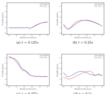
Snapshots of the simulation results are presented in Figs. 1 and 2. The first figure shows the results for a small boundary input excitation. In this case, the difference between the two responses are undistinguishable, since the excitations is small. The second figure shows the snapshots for a large excitation. As expected, differences between the linear and nonlinear responses are observed for large amplitudes.

B. 2D controlled model

The second simulation presented consists in the 2D model, assuming the following initial conditions:

αq(t = 0, r, θ) = h(t = 0, r, θ) = cos(πr/R) cos(2θ) ,

α α

αp(t = 0, r, θ) = ρuuu = 0 .

(40) The boundary conditions are assumed to be:

u∂(t, s) = 0 , t≤ 0.5s , u∂(t, s) =−k ( y∂(t, s)− y∂0 ) , t > 0.5s , (41)

(6)

0 .0 0.2 0.4 0.6 0.8 1.0 Radialcoordinate[m] 0.9998 1 .0000 1.0002 1.0004 1 .0006 1.0008 1.0010 1 .0012 1.0014 F lu id H e ig h t[ m ] Nonlinear Linear (a) t = 0.125s 0 .0 0.2 0.4 0.6 0.8 1.0 Radialcoordinate[m] 0.9998 1 .0000 1.0002 1.0004 1 .0006 1.0008 1.0010 1 .0012 1.0014 F lu id H e ig h t[ m ] Nonlinear Linear (b) t = 0.25s 0.0 0.2 0.4 0.6 0.8 1.0 Radialcoordinate[m] 0.9998 1.0000 1.0002 1.0004 1 .0006 1.0008 1.0010 1 .0012 1.0014 F lu id H e ig h t[ m ] Nonlinear Linear (c) t = 0.375s 0.0 0.2 0.4 0.6 0.8 1.0 Radialcoordinate[m] 0.9998 1.0000 1.0002 1.0004 1 .0006 1.0008 1.0010 1 .0012 1.0014 F lu id H e ig h t[ m ] Nonlinear Linear (d) t = 0.5s

Fig. 1: Snapshots for the 1D simulation using a small amplitude harmonic excitation at the boundary

i.e., the feedback control law proposed in Section IV is activated after 0.5 s of simulation.

As in the one-dimensional reduced simulation model, continuous Galerkin elements with 1st-order Lagrange poly-nomials are used for approximating the q variables and dis-continuous Galerkin elements with 0-order Lagrange poly-nomials are used for approximating the p variables.

The system Hamiltonian as well as the Lyapunov function are presented as a function of time in Fig. 3. Note that during the first 0.5 s of the simulation, both the Hamiltonian (total energy) and the Lyapunov function are constant. After 0.5 s, the Hamiltonian reduces and oscillates until converging to the new energy minimum. The Lyapunov function monotonically decreases towards zero. Snapshots of the simulation are presented in Fig. 4.

VI. CONCLUSIONS AND FURTHER WORK This paper presented a port-Hamiltonian representation of the 2D nonlinear Shallow Water Equations in polar coordi-nates, in order to simulate a water basin with boundary wave-generators. Thanks to the use of polar coordinates, a 1D reduced model was obtained, assuming revolution symmetry of both the initial conditions and the boundary actuation. The 1D and 2D equations were approximated in finite dimension using the Partitioned Finite Element Method, that preserves the port-Hamiltonian system structure and can be implemented in well-established Finite Element software. Nonlinear time-domain simulations were performed. So far, a simple boundary feedback control law was tested in the numerical simulations, being able to dissipate the water waves.

Thanks to the port-Hamiltonian structure of the system, further work should focus on the interactions that happens

0 .0 0.2 0.4 0.6 0.8 1.0 Radialcoordinate[m] 0 .9 1 .0 1 .1 1.2 1.3 1.4 F lu id H e ig h t[ m ] Nonlinear Linear (a) t = 0.125s 0 .0 0.2 0.4 0.6 0.8 1.0 Radialcoordinate[m] 0 .9 1 .0 1 .1 1.2 1.3 1.4 F lu id H e ig h t[ m ] Nonlinear Linear (b) t = 0.25s 0.0 0.2 0.4 0.6 0.8 1.0 Radialcoordinate[m] 0.9 1.0 1 .1 1 .2 1 .3 1.4 F lu id H e ig h t[ m ] Nonlinear Linear (c) t = 0.375s 0.0 0.2 0.4 0.6 0.8 1.0 Radialcoordinate[m] 0.9 1.0 1 .1 1 .2 1 .3 1.4 F lu id H e ig h t[ m ] Nonlinear Linear (d) t = 0.5s

Fig. 2: Snapshots for the 1D simulation using a large amplitude harmonic excitation at the boundary

0.0 0.5 1.0 1.5 2.0 2.5 3.0 Time (s) 15600 15800 16000 16200 16400 T ot al E n er gy (J )

(a) Total energy (Hamiltonian)

0.0 0.5 1.0 1.5 2.0 2.5 3.0 Time (s) 0 5 10 15 20 L ya p u n ov F u n ct io n (J ) (b) Lyapunov function

Fig. 3: Total energy and Lyapunov Function

on the boundary with the wave-generator actuators. Dynamic models of these actuators can be easily coupled to the SWE through the boundary-ports. Following this idea, other feedback boundary control strategies could be implemented, such as control by interconnection and impedance control.

REFERENCES

[1] R. R. Robles and J. P. Serrano, “Sloshing mechanical model for stability and handling qualities evaluation of the C295 aircraft with the OSD system,” in Proceedings of 29th Congress of the International

Council of the Aeronautical Sciences, (St. Petersburg, Russia), 2014.

[2] M. Clifford, C. Horton, and J. Schmitz, “Swafs: Shallow water analysis and forecast system,” in Proceedings of OCEANS’94, vol. 3, pp. III– 82, IEEE, 1994.

[3] Y.-S. Cho, D.-H. Sohn, and S. O. Lee, “Practical modified scheme of linear shallow-water equations for distant propagation of tsunamis,”

Ocean Engineering, vol. 34, no. 11-12, pp. 1769–1777, 2007.

[4] J. Scruggs and P. Jacob, “Harvesting ocean wave energy,” Science, vol. 323, no. 5918, pp. 1176–1178, 2009.

[5] P. Warnitchai and T. Pinkaew, “Modelling of liquid sloshing in rect-angular tanks with flow-dampening devices,” Engineering Structures, vol. 20, no. 7, pp. 593–600, 1998.

[6] H. A. Sch¨affer, “Second-order wavemaker theory for irregular waves,”

(7)

x[m] −1.00 −0.75 −0.50−0.250.000.250 .500.751.00 y[m ] −1.00 −0.75 −0.50 −0.25 0.00 0.25 0.50 0.75 1.00 h [m ] 0.93 0.95 0.97 0.99 1.01 1.03 1.05 1.07 1.09 1.11 Fluid Height (a) t = t0 x[m] −1.00 −0.75 −0.50−0.250.000.250 .500.751.00 y[m ] −1.00 −0.75 −0.50 −0.25 0.00 0.25 0.50 0.75 1.00 h [m ] 0.93 0.95 0.97 0.99 1.01 1.03 1.05 1.07 1.09 1.11 Fluid Height (b) t = 1/7 tend x[m] −1.00 −0.75 −0.50−0.250.000.250 .500.751.00 y[m ] −1.00 −0.75 −0.50 −0.25 0.00 0.25 0.50 0.75 1.00 h [m ] 0.93 0.95 0.97 0.99 1.01 1.03 1.05 1.07 1.09 1.11 Fluid Height (c) t = 2/7 tend x[m] −1.00 −0.75 −0.50−0.250.000.250 .500.751.00 y[m ] −1.00 −0.75 −0.50 −0.25 0.00 0.25 0.50 0.75 1.00 h [m ] 0.93 0.95 0.97 0.99 1.01 1.03 1.05 1.07 1.09 1.11 Fluid Height (d) t = 3/7tend x[m] −1.00−0.75 −0.50 −0.250.000.250 .500 .751.00 y[m ] −1.00 −0.75 −0.50 −0.25 0.00 0.25 0.50 0 .75 1.00 h [m ] 0.93 0.95 0.97 0.99 1.01 1.03 1.05 1.07 1.09 1.11 Fluid Height (e) t = 4/7 tend x[m] −1.00−0.75 −0.50 −0.250.000.250 .500 .751.00 y[m ] −1.00 −0.75 −0.50 −0.25 0.00 0.25 0.50 0 .75 1.00 h [m ] 0.93 0.95 0.97 0.99 1.01 1.03 1.05 1.07 1.09 1.11 Fluid Height (f) t = 5/7 tend x[m] −1.00−0.75 −0.50 −0.250.000.250 .500 .751.00 y[m ] −1.00 −0.75 −0.50 −0.25 0.00 0.25 0.50 0 .75 1.00 h [m ] 0.93 0.95 0.97 0.99 1.01 1.03 1.05 1.07 1.09 1.11 Fluid Height (g) t = 6/7 tend x[m] −1.00−0.75 −0.50 −0.250.000.250 .500 .751.00 y[m ] −1.00 −0.75 −0.50 −0.25 0.00 0.25 0.50 0 .75 1.00 h [m ] 0.93 0.95 0.97 0.99 1.01 1.03 1.05 1.07 1.09 1.11 Fluid Height (h) t = tend

Fig. 4: Boundary control using a proportional gain tend= 3[s]

[7] J. Spinneken and C. Swan, “Second-order wave maker theory using force-feedback control. Part I: A new theory for regular wave gener-ation,” Ocean Engineering, vol. 36, no. 8, pp. 539–548, 2009. [8] J. Spinneken and C. Swan, “Second-order wave maker theory using

force-feedback control. Part II: An experimental verification of regular wave generation,” Ocean Engineering, vol. 36, no. 8, pp. 539–548, 2009.

[9] S. Naito, M. Minoura, K. Tanaka, H. Sakashita, et al., “Evaluation of performance of new wave-making basin,” in The Ninth International

Offshore and Polar Engineering Conference, International Society of

Offshore and Polar Engineers, 1999.

[10] K. Maeda, N. Hosotani, K. Tamura, and H. Ando, “Wave Making Properties of Circular Basin,” in Proceedings of the 2004 International

Symposium on Underwater Technology, pp. 349–354, IEEE, 2004.

[11] D. Ingram, R. Wallace, A. Robinson, and I. Bryden, “The design and commissioning of the first, circular, combined current and wave test basin,” in OCEANS 2014 - TAIPEI, vol. 9637, pp. 1–7, IEEE, apr 2014.

[12] D. R. Noble, T. A. D. Davey, H. C. M. Smith, P. Kaklis, A. Robinson, and T. Bruce, “Spatial variation in currents generated in the FloWave Ocean Energy Research Facility,” Proceedings of the 11th European

Wave and Tidal Energy Conference, pp. 1–8, 2015.

[13] S. Salter, “Absorbing wave-makers and wide tanks,” in Proceedings of

the conference on Directional Wave Spectra Applications, (Berkeley,

California), 1981.

[14] J. Spinneken, M. Christou, and C. Swan, “Force-controlled absorption in a fully-nonlinear numerical wave tank,” Journal of Computational

Physics, vol. 272, pp. 127–148, 2014.

[15] I. Gyongy, T. Bruce, and I. Bryden, “Numerical analysis of force-feedback control in a circular tank,” Applied Ocean Research, vol. 47, pp. 329–343, 2014.

[16] V. Duindam, A. Macchelli, S. Stramigioli, and H. Bruyninckx,

Model-ing and Control of Complex Physical Systems: The Port-Hamiltonian Approach. Berlin, Heidelberg: Springer Berlin Heidelberg, 2009.

[17] A. J. van der Schaft and D. Jeltsema, “Port-Hamiltonian Systems

Theory: An Introductory Overview,” Foundations and Trends⃝ inR Systems and Control, vol. 1, no. 2, pp. 173–378, 2014.

[18] T. J. Courant, “Dirac manifolds,” Transactions of the American

Math-ematical Society, vol. 319, pp. 631–661, feb 1990.

[19] A. J. van der Schaft, “Port-Hamiltonian Systems: Network Modeling and Control of Nonlinear Physical Systems,” in Advanced Dynamics

and Control of Structures and Machines (H. Irschik and K. Schlacher,

eds.), pp. 127–167, In: Advanced Dynamics and Control of Structures and Machines. Springer, 2004.

[20] B. Hamroun, L. Lefevre, and E. Mendes, “Port-based modelling and geometric reduction for open channel irrigation systems,” in

Proceedings of the 46th IEEE Conference on Decision and Control,

(New Orleans, LA, USA), pp. 1578–1583, IEEE, 2007.

[21] B. Hamroun, A. Dimofte, L. Lef`evre, and E. Mendes, “Control by Interconnection and Energy-Shaping Methods of Port Hamiltonian Models. Application to the Shallow Water Equations,” European

Journal of Control, vol. 16, pp. 545–563, jan 2010.

[22] R. Pasumarthy, V. R. Ambati, and A. J. van der Schaft, “Port-Hamiltonian discretization for open channel flows,” Systems & Control

Letters, vol. 61, no. 9, pp. 950 – 958, 2012.

[23] F. L. Cardoso-Ribeiro, D. Matignon, and V. Pommier-Budinger, “A port-Hamiltonian model of liquid sloshing in moving containers and application to a fluid-structure system,” Journal of Fluids and

Struc-tures, vol. 69, no. December 2016, pp. 402–427, 2017.

[24] F. L. Cardoso-Ribeiro, D. Matignon, and L. Lef`evre, “A structure-preserving Partitioned Finite Element Method for the 2D wave equa-tion,” IFAC-PapersOnLine, vol. 51, no. 3, pp. 119–124, 2018. [25] F. L. Cardoso-Ribeiro, M. D., and L. Lef`evre, “A Partitioned

Finite-Element Method (PFEM) for power-preserving discretization of open systems of conservation laws,” arXiv:1906.05965, 2019.

[26] M. S. Alnæs, J. Blechta, J. Hake, A. Johansson, B. Kehlet, A. Logg, C. Richardson, J. Ring, M. E. Rognes, and G. N. Wells, “The FEniCS Project Version 1.5,” Archive of Numerical Software, vol. 3, no. 100, 2015.