Coordinating aggregate and detailed scheduling decisions in the one machine job-shop; I-theory,

LIBRARY OF THE

MASSACHUSETTS INSTITUTE

ALFRED

P.

SLOAN SCHOOL OF

MANAGEMEN

COORDINATING AGGREGATE AND DETAILED SCHEDULING

DECISIONS IN THE ONE MACHINE JOB-SHOP: I-THEORY

L. Gelders and P. R. Kleindorfer

•

b^rt

600-72 _{April, 1972}

MASSACHUSETTS

INSTITUTE

OF

TECHNOLOGY

50

MEMORIAL

DRIVE

BRIDGE,

MASSACHUSETTS

COORDINATING AGGREGATE AND DETAILED SCHEDULING

DECISIONS IN THE ONE MACHINE JOB-SHOP: I-THEORY

L. Jelders and P. R. Kleindorfer

600-72 April, 1972

00.

600-75

Dewe

RECEIVEO I JUN

g

1972 '*^-'-T._LIBRARIES

COORDINATING AGGREGATE AND DETAILED SCHEDULING

DECISIONS IN THE ONE MACHINE JOB-SHOP: I-THEORY

by

L. Gelders and P. R. Kleindorfer

ABSTRACT

This research presents a formal model of the one machine job

shop scheduling problem with variable machine and labor capacity.

Pri-mary interest is focused on the trade-off between overtime and detailed scheduling costs. The detailed scheduling problem considered is minimiz-ing the sum of weighted tardiness and weighted flow-time costs for a given

capacity plan (e.g., a given overtime schedule). Sequence theory results

are generalized to this case where possible. Various lower bounding struc-tures for the problem are analyzed and a preliminary branch and bound

al-gorithm is outlined. Several interesting features of the algorithm and bounding structures are illustrated by an example. Extensions of the re-sults to more complex environments are discussed.

1. Introduction

This paper addresses the problem of coordinating aggregate and

detailed scheduling decisions in a job-shop environment. Typically, the aggregate planning level determines a medium-run capacity strategy for

workforce, overtime, and shifts. Given this plan, the detailed

schedul-ing problem is concerned with minimizing operating costs subject to quali-ty control constraints. There is clearly a tradeoff between capacity costs and the direct costs incurred in scheduling individual jobs to activity centers. The problem of concern here is the determination of reasonable procedures for resolving this tradeoff between aggregate and detailed level

costs.

As a first step in addressing the combined aggregate-detailed scheduling problem discussed above, this research studies the problem in a

one machine job-shop. In this context, the problem becomes one of deter-mining an overtime plan and job processing sequence which minimizes the sum

of overtime costs and direct job costs due to tardiness, in-process

inven-tory, and other flow- time related costs. Following the framework of Conway,

et. al

.

[1967], certain general results are first derived for this problem.

On the basis of these, a branch and bound algorithm is presented for solving problems of modest size. Computational results and a discussion of the uses

of the framework presented in structuring and evaluating procedures for more realistic problem settings are given in a companion paper [6].

Two bodies of literature are relevant to this research -- job-shop scheduling and aggregate planning. We first briefly review relevant aspects

of the literature on job-shop scheduling.

-2-much attention in the secheduling literature. For some regular measures of performance, elegant and simple results are known, e.g. the shortest

processing time rule for minimizing mean flow time. However, no such results are available when certain alternative performance measures are

used. The detailed sequencing problem of interest in this paper falls in-to this latter category. The sequencing problem considered here is formu-lated as follows:

Problem A Minimize Z (p-T. + h-F.)

j = job index

N = job set = {1,...,n}

C. = completion time of job j

d. = due date of job j (d. >_ 0)

T. = _tardiness of job j = Max (0, C- - d.) p. = tardiness penalty per unit time (p- >_ 0) r. = _ready time or release date of job j (r. >_ 0) F. = flow time of job j = C. - r

.

h. = holding cost penalty per unit time (h. >_ 0).

The objective in Problem (A) is to minimize tardiness and flow-time related costs. When h = o for all jobs, the weighted tardiness problem re-sults, various forms of which have been studied by McNaughton 02], Schild and

Fredman [13,1<|, Held and Karp [9], Elmaghraby [4], Emmons [5], Srinivasan [19] and others. An efficient branch and bound algorithm for this case has been

-3-Turning now to the aggregate planning literature, a wealth of models and results is available^. However, on the normative side at least,

little of this work has been related to the job-shop context. A more seri-ous lacuna is the fact that only recently have these resutls been related to the problem of coordinating aggregate and detailed scheduling^. A heur-istic coupling procedure resembling the structure of the algorithm in this paper has been developed and evaluated in a simulated job-shop environment by Green [7]. Recent work of Shwimer [16] has further corroborated the benefits to be gained by coordination of aggregate and detailed scheduling decisions in the job-shop context.

In this research we assume a simple functional form for aggregate costs. Generalization will be discussed below. Under the hypothesis of a

homogeneous and constant workforce, the aggregate costs here are represented

as follows.

k=l ^ ^

K = _{number of periods} in planning horizon

X. = hours of overtime in period k = 1,2,...,K;

b, = unit cost of over time in period k = 1,2,...K.

In the next section we couple Problem (A) with these aggregate

See Chapters 5 - 7 of Buffa and Taubert [1] and references therein.

See Newson [12] and references therein for some normative results for production processes making standardized products.

-4-costs and related constraints to obtain the combined aggregate-detailed scheduling problem of interest. In Sections 3 and 4, a bounding structure

is developed for solving the combined problem. Section 5 specifies a

first-cut branch and bound algorithm for the problem and gives an

illustra-tive example. Conclusions and directions for further research are

2. Problem Formulation

2.1. Capacity Plans and Sequencing Results

Our initial aim is to delineate the set of capacity plans of interest here and a convenient parameterization of these plans.

Let a planning horizon H >_ be given. Let q(T) >^ be the

instantaneous processing rate of the machine (or activity center) at time

Te[0, H]. The trajectory

{qd/rxe

[0, H]} is called a capacity plan.

We will be primarily concerned with a special case of these capacity

plans, for which q(T) either equals 1 or for all x. In this case either the machine is available (qCx) = 1) or not (q(T) = 0). When it is available, processing is at a uniform rate. These capacity plans will be called simple overtime plans. In order to specify such plans more precisely, we proceed

as follows.

Partition the interval [0, H] into K disjoint periods where the start of period k is denoted by a. , k = 1,...,K and where = a, <_ ...

±

a^^-, = H. Let {X . :k = 1,...,K} be a set of non-negative integers, x .

is called the maximum permissible overtime level in period k.

Let {p|,:l< = 1,...,K} be a set of non-negative integers, where P|^

connotes period k regular time. It is assumed that

(2-1)

°k ^ Pk -^

^mk:i

_'^k+P

^ =

'-•-K,

so that the maximum permissible overtime level fits into period k.

-6-(2.2) X = {xeE :x = (Xp...,x,^); x,^e{0, _K-.-.x^^k):

K n

k=1 ^ ^ j=l -^

The last requirement in (2.2) assures that enough overtime will be allocated to accomplish all jobs within [0, H]. It is assumed that X ^ 0, i.e.

K n

k=l ^ ^^ j=l ^

For each xeX define a simple overtime plan as follows:

(1

if a,^

£

T

£

a|^ + P|^ + X|^, k = 1,...,K;

else.

Figure 1 represents a typical simple overtime plan. Since the regular time p. is assumed fixed for all k, any feasible vector of overtime levels XeX determines a unique capacity plan. In the sequel we will represent simple overtime plans by their corresponding overtime level vector x

-7-<](^,^) ,.

Tint

^l^

k

toi.e ^em»ot>

P

I

K

a-,«o _<a

_^*

ft. '^^ A Simple Overtime Plan

Figure 1

%^±

Given a simple overtime plan q(T,x) the completion times for any

preemptive schedule can be found via the usual procedure of "loading" job

processing times onto the given graph of q(T,x). To make this loading pro-cedure more precise we Introduce the cummulatlve capacity curve yij) as

;2.4) y(T) =

I

q(T')dT'

and define the completion time for processing y units of work starting at

-8-(2.5)

C=

inf {t' e y''(Y + y')}, y' =

_yd).

where y~ (y') =

_d'

>_0:y(T') = y'}. Figure 2 illustrates the relationship of the loading procedure to the use of the cumulative capacity curve in de-termining completion times. In the example illustrated in Figure 2 n = 2, t-, = tp = 2, and the schedule of processing requirements given is: {1 unit, job 1; 2 units, job 2; 1 unit, job 1}.

DLC

\

DUE

6

_C

Illustrating Completion Time Determination

-9-Note that the schedule derived is preemptive resume (see

[2]).

That is, processing on a job interrupted by another job or by a non-pro-ductive period can be resumed without additional cost or time. We assume

in what follows that all processing has this preemptive resume property

.

Generalizing the above example, let (I-i,

Y^

I2, Y^,..., !_, Y }

be a sequence of processing and idle time requirements, where I- is the idle time preceeding the ith processing segment Y-. It is readily veri-fied that the loading procedure above corresponds to the following:

(2.6) y. = y(C._^ + !•) i = 1,..., P

(2.7) C. = inf {t' e

y'^y.

+ Y.)}

^'ic.-i^^-where Cq = and C- is the completion time of processing segment Y-. In the case where more than one non-zero processing rate is

pos-sible, the t- would be in standard hours of capacity. Any given schedule of standard hour processing and idle time requirements would then be

trans-lated into (calendar) completion times sequentially by (2.6) and (2.7).

Assuming a quite general (continuous, non-decreasing) cumulative

capacity curve it is possible to generalize certain results of sequence theory. Specifically, Conway et. al.

[2]

prove the following properties for the case when q(T) = 1 for all t and r- = for all j.

(PI) When scheduling against a regular measure of oer-formance, inserted idle-time need not be considered.

-10-(P2) When scheduling against a regular measure of performance, preemption need not be considered.

(P3) The maximum flow time F is independent of the max

job sequence.

(P4) The SPT-rule minimizes mean flow time F.

(P5) The weighted SPT-rule minimizes weighted flow time

. "J

Fj.

Properties (PI) - (P4) can be readily verified. The proofs of these properties are analagous to the corresponding proofs in Conway et. al. [2 ]. It should be noted that these proofs are constructive. In the case of (PI) the proof indicates that one should simply eliminate the idle time by left shifting all jobs as far as possible. In the case of (P2) one can construct from a given preemptive schedule S a non-preemptive

schedule which is at least as good by sequencing the jobs in order of their completion times in S (i.e. the job with largest completion time in S goes last, the job with second largest completion times in S goes next to last, etc.). As an exai^ple, appendix 1 gives a proof of (P4). Of course, none of these properties necessarily hold when jobs do not arrive

simultaneously, though one could still consider the problem of finding

the best non-preemptive schedule.

The following example shows that (P5) does not generally hold even in the case of simple overtime plans.

Example: Let n = 2 with t^ = 8 t^ = 12

(2.8) q(

'{;

-n-10 < T

£

20, T >^ 30

1

T

1

10. 20

_£

T < 30

It can be verified that the weighted SPT sequence {2, 1} has completion times C-j = 30, C^ = _{22 with} E oj-F- = 274. However, the sequence {2, 1} has completion times C^ = 30, C2 = 8 with E w-F- = 242.

On the basis of (PI) and (P2) above we may restrict our attention when r. = for all j, to the n! permutation schedules (see [2], p.25) re-presented by the set of permutations n = {Tr:N -> N; 7r(i) = fT(-j) _implies

i = j}. In this case, since inserted idle time is not considered, the completion times _{for given yix) and} tt e n are obtained from (2.6), (2.7)

as follows:

(2.9)

_c^i)

=

_{j?f^/^'^y-Vt,„));}

<'-^°'

^0 = ^"^.(J-l)) J = 2. ,n;

-

tt(J-I)

^^(j)' ^-^(j) ^^^ ^^^ proces^ng time and completion time respectively of the job in jth position under the given permutation tt.

-12-2.2 Statement of the Problem

The global problem to be solved is as follows:

K N (2.12) Minimize G(x,7r) = Z b.x,^ + E (p.T. + h-F.) X, n i<=i ^ ^ j=l J J J J =

_J^Vk

^

J/Pj

"^^^^°' ^j -'j^ ' 'j^^J -'j^^

where X is given by (2. 2),

His

the set of permutation schedules, and where

C

is determined by (2.4), (2.9) - (2.11).

-13-3. Reduction of the Solution Set

3.1 Dominance Relation for Overtime Vectors

When all the .lobs are simultaneously available and the unit cost of overtime is constant, it is not necessary to enumerate all the

feasible overtime vectors. We will prove that for a given total amount

of overtime z, one particular vector x necessarily dominates all the overtime vectors x with the same value of z.

Lemma 3.1 _(Dominance Relation):

Let X, x'

eX

and suppose the followinq hold:

a) x^ = x! for k _f i, m;

b) X, > x' and x < v' with j, < m;

c)

_hv

=

_hi

= z;

Then if b, = b, k = 1,...,K; 6(x,7t) <_'^(x',Tr), tt e n, where G is given by (2.12).

Proof: Let tteR be arbitrary and let {C.:jeN} and {C.':jeN} be the completion

times under tv for the given overtime vectors x and x' respectively. From

conditions a-c above and (2.3)-(2.4) it follows that

y(T)=y'(T)

for < T < a^ + Pjj^ + x^;

y(T)

>y'(T)

for

a^+

Pj^ + x^ < t < a^ + P^ +

x-yd)

= y'(T) for a^ + _p^ + x^; < T < H;

where y(T), y'(T) are the cumulative capacity curves corresponding to x

14-In particular, the above implies y(T) >_y'(T) for t>_ 0. Therefore, from (2.9)-{2.n), C. < C.' for all jeN. Since Zb.x. = Sb.x. ' = bz and

Jj

kk

since weighted tardiness and weighted flow-time are regular measures of

performance, G(x,Tr) < G(x',Tr). QED

Lemma 3.1 implies that once a given total amount of overtime z is fixed, the overtime should be moved as early as possible in the time horizon. Thus for given z, one need only consider the following overtime vector.

(3.1) X? = min(z,Xj^^) k-1

x^ = min(z - Z x?,Xj^,^), k = 2,...,K.

As a result, one need only consider the set of feasible total

overtime levels given by

(3.2) Z = {z = z . .z _.„ + _1, ...,z }

min

mm

' _max

where, from the requirement in (2.2) that sufficient overtime be scheduled to process all jobs,

(3.3) z^.^ = Max{ EE tt. - Z p. ,0j j=l ^ _k=l ^

The value of z^^ is determined from the maximum permissible overtime levels, x^j^, and the observation that there is no need to add overtime in periods after which the last job is completed. Thus, z

max is given by

15-K*

where K*

£

K is the earliest period for which

K* n

(3.5) Z (p. + X

J

> I t. k=l ^ ^^ j=l ^ holds.

Given the above we define

(3.6) g(z,7T) = Min {G(x,u):xeX,Ex. = z) = G(x°,7t) k ^

where x° is given by (3.1).

3.2 Generalization of Elmaghraby's Lemma and Shwimer's Theorem A.

It is of interest to note that Shwimer's Theorem A [15] may be generalized to the present problem. In particular it can be shown that for any two jobs i and j, for which:

.< t. .< t

.

^ ^ ^] < dj _{There exists} an optimal schedule

- in which i precedes j.

p. , p. >.

h. ^ h. ^

The detailed proof is analogous to Shwimer's argument and is available from the authors.

Shwimer's original proof assumes q(T) = 1, t>0, and h. - 0,

16-Of more importance from a computational point of view is the following generalization of Elmaghraby's Lemma [4 ], the proof of which follows Elmaghraby's original argument and which is also available from the authors.

Lemma 3.2

Suppose h. = _0, r. = _0, j = l,2,...,n. Let N = N1UN2,

J J

NinN2 =

4-Suppose that TT(j)e{k+l....,n}, jeNjcN (i.e. jobs in N2 are

scheduled last under tt). If

(3.7) E t. <

J(d^

) where d^ = Max = d.*

Then, there exists a Tr*en such that iT*(j)e{k+l ,...,n}, J£N2

n n

and 7r*(j*) = k, and Z p.T.(tt'^) < I

pJAt\)

for Tren satisfying

j=l J J J

j=H

"^

Tr(j)e {k+1. n}, JeNj.

The only difference between the above and Elmaghraby's origina'

formulation is that y(dj,, ) replaces d^, in the hypothesis (3.7). When

q(T) =

1,¥t,

then y(d|. ) = d|.^ , and the original lemma results from

-17-3.3 Tree Exploration Scheme

The set of admissible solutions may be represented in a tree search scheme as follows:

level

level 1

level 2

job j in first position

Figure 5: Tree Structure

Obviously, a "Shwimer-like" algorithm [15] may be used for the exploration of nodes on level 1. Shwimer's algorithm may be easily gen-eralized for these circumstances (variable capacity and h. ^ 0). So, the current problem may be solved by using this algorithm after a complete enumeration of the nodes on level 1. In the next section, however, we will develop an alternative algorithm which calculates strong lower bounds

for the nodes on level 1. The method proposed provides automatically

4. Lower Bounding Procedure for Variable Capacity Plans

4.1 Introduction

The problem of concern here is to establish lower bounds on the scheduling costs of a set of jobs processed under a given capacity plan

and for an objective function of the following form:

(4.1) Min Z {p. Max(C. - d., 0) + h.F.}

-i jeN -J J J J J

where

A

is the set of preemptive schedules subject to W.:^r. (job processing may not begin until after job release). When all jobs are simultaneously available, (PI) and (P2) in 2.1 above indicate that i6 in (4.1) can be replaced by the subset n of)& without changing the optimal value of the

objective function. It is clear, however, that in the general case of intermittent job arrivals (r. f 0) preemption and inserted idle time must be considered (see

[2],

p. 69).

The bounding procedure established below holds under any capacity

plan and for r. f 0. For convenience, we will restrict the formulation and the proof of our procedure to the problem of primary concern in this study, i.e. r. = for all j and only simple overtime plans.

Generali-zations to these other cases will be apparent from the comments and corollaries.

4.2 A Lower Bounding Problem

Consider the problem {?).

Problem (P): Find

(4.2) Min E p, Max(C, - d,, 0) ^ Min I p. Max(C. - d., 0)

-19-We now formulate a transportation problem (P-1). The

under-lying idea is that the above scheduling problem may be seen as a

transportation problem in which capacity units (available in different time periods) have to be shipped to different jobs.

Problem (P-1):

Consider any arbitrary division of the time horizon H into

timeslots i = 1,2,3,..

.,v-l,v. Such a partitioning of H can be represented

by a set of discrete points T = _(ti,t2,t3,...,t

| = ti<t2<_...<t <H)

which represent the starting points of the corresponding timeslots.

The problem (PI) then is the following: V n (4.3) Find: L(q,T) = Min E E a. .w. . i=l j=l ^J ^^ n subject to: Z w. . < s ., i = 1,...,v; j=l ^^

~

" S w. . = t., _j = l,...,n; j=l ^^ J w.j

_^0,

all i,j;

where w. . = amount of capacity used by job in timeslot i

;

Ti+l

s. = capacity supply in timeslot i = / q(T')dT';

(4.4)

t. = capacity demand of job j = processing time of job j; and

a.-. =/{! + [(t. - _d.)/t.]}p. for all slots i with t.>d

.

1J I ' _{J J J}

'J

^ _elsewhere

-20-It is clear that,when a simple overtime plan is given, for any arbitrary partition T, a unique problem (PI) may be derived from Problem (P). It is also clear that the set of schedules i^corresponding to the feasible set of (PI) contains both preemptive and non-preemptive schedules

4.3 Lemma

M "

If E y <t, then E yy <M.t

y=l ^ y=l ^

M M M

Proof: l \iy <

ZMy

=MZy

<M.t y=l ^ y=l ^ y=l

^~

4.4 Proposition

Suppose a simple overtime plan q(T,x) has been fixed. Then the

optimal solution to problem (PI) is a lower bound on the optimal solution of (P) for any arbitrary partition T of the time horizon H.

Proof: (i) Clearly any feasible solution in (P) is feasible in (PI). Therefore it suffices to prove (ii).

(ii) The cost associated with a feasible solution of (P) is always underestimated by the corresponding solution of (PI).

Consider an arbitrary schedule in S and the corresponding solution llw^.-llof (PI). The contribution of job jeN to the total cost

of problem (P) is p.T.. Let us now calculate the contribution of job j

to the total transportation cost of (PI). If p. = the costs in both (P) and (PI) are zero. We therefore assume p.>0.

-21-Consider two time axes, the original one (partitioned following

T) and an axis (d. + yt.). u = _{0,1,2,..., with origin} d.. In the sequel we will represent a timeslot by its index i or by a pair (t.,1.^,)

fiat-4

—

L . 'P**! .

J

—

____

1 ,

sag

, - I

La.

I

7

T^=0 T2 Ji+1 I I y=0 ^ij 'I 2 , 3 I ^2 ' ""3 M 'm+1 H ^j* "tj M+1

^+1

Suppose that the last assignment of capacity with relation to

job j takes place in timeslot m. The first timeslot with ajj i^ and

w. . ?* is called i. Then, the contribution of job j to the total trans-portation cost is:

m m

m

Consider now $ = U (t-,!..-,) and let us partition $ in mutually exclusive

i=i!,

sets a with y

(4.6)

%=

UT.,T.^^)la.j = _ypj},

y=

1,2,

m M+1

Then from (4.4) $ = U (t-,t.^i) = U a

^=l y=l

From (4.5) and (4.6) it follows that

m M+1

L.=

Ea..w..=

Z Z a..w.. or (4.7) ^=l M+1 y=l iea y M+1 L. = Z Z yp.w. . = p. Z y Z w. .

-22-Now, let us define

(4.8) y = z w.

.

^ _lea

^

y From (4.7) and (4.8) we derive

M+1 M

We know that:

M M

lly = I Z w. < t. - _Z w..

y=l^ U=l

iea/J

^ iec^^^ ^J

(4.10)

^f/y ^

^j

-^M.l

Applying Lemma 4.3 to equation (4.10) yields

(4.11)

_^f/^ylf^^tj

_-y^,^)

It follows from (4.9) and (4.11) that

(4.12) _k-

lP,{M(t,

- _y„,,)

MM

+ 1) _M.i>

'M+1 M+1

By (4.12) and the definition of y^.-,, we therefore obtain

M+1

4

(4.13)

_^

_l"tj*y„,,

'Mtj*

£

w.j+w^j

V

m Now since Mt. + E w. . < t - d., J ,• 1J

—

m J ^i^^m (4.14; _-f- < T + w . - d. Pj

-

m mj J

-23-But T + w_. - cl.<C. - d. = T.. Equation (4.14) therefore yields L.<p.T., Since j was arbitrary 2

1-^12

p.T. for any schedule i" _i. Thus

jeN -^ _jeN -J _^

(4.15) L(z,T) < Min Z p.T. < Min E p.T. (Q.E.D.)

^

jeN ^ ^ _{n jeN} J "^

4.5 Corollaries

4.5.1 Let us consider problem (P') defined as follows:

Min Z h.F. = Min Z h.F.

n _jeN "J J

_^

_jeN ^ ^

Then, the optimal solution of (PI) is a lower bound on the optimal solution of (P') when using the following transportation costs;

(4.16) a.j. ^ {1 + [T^-/tj.]}hj for all x.

Proof: The assertion follows immediately from (4.2) and (4.4) by putting

d. = and p. = h..

4.5.2. Since (PI) is a linear program, the proposition of

4.4 holds also for bounding the sum of penalty costs and holding costs,

i.e. for

Min Z (p,T. + h.F.) n JeN ^

J ^ ^

The cost coefficients are then given by

(4.17) a.j ^/{l + [(t. - dj)/tj]}Pj + {1 + [Ti/tj]}h. for T.>d.

-24-4.5.3. The procedure described above may be used for bounding any convex piece-wise linear cost function of completion time as such a function may be considered to be the sum of linear penalty functions of the form con-sidered in section (4.4). The individual cost matrices simply add together,

4.5.4. The lower bounds obtained by this procedure are clearly a function

of T. Now consider two partitions T and T' of H such that

T

= _{{-^I'^e-'-^n'Vl}

...^v^ and T' = {t^'12'•..t^'. ..t' }such that

(4.18) T^. = T.' for i = l,...,n

"^n "

V-

^'n+1

-

""'n+Z ••'

-

^'n+p+1 "

Vl

T^ = t'.^ for i = n+l,...,v

It follows from the definition of the cost coefficients a. • in (4.4) that

L(z,t)

£L(z,T').

Thus the finer the time divisions the better the

bounds.

4.6 Extensions

The results obtained above may be generalized in the following way:

4.6.1 When dealing with other than simple overtime plans, it can be verified that an analogous bounding procedure can be used. It suffices to multiply the costs a^ . by _a factor X^ =

^^^

,y

provided that

Max q(T) >^ 1

-25-4.6.2 The generalization to the case of r. ^ is obvious. The cost coefficients to be used are

6,j{l ^ [(T. - d.)/t.]}p. . {1 . [(T. - r./t.]}h. (4.19)

_,..4i

'°^^i^^J

M for T.< r. where t 1 if x- > d. 6.-. = 1

-

J ^^

₍₀

_otherwise

The detailed proof of 4.6.1 and 4.6.2 is completely similar to the proof given under 4.4, and it is available from the authors.

4.6.3 Let y(x,S) be the detailed sequencing costs for a given overtime vector X and schedule Se^, i.e.

(4.20) y(x,S) = Z (p.T. + h.F.)

j=l ^ ^ ^ ^

Suppose x' < x" (i.e. X||, < xj;, k = 1,...,K). Let S' and S" be the optimal

schedules corresponding to x' and x" respectively. Clearly y(x',S') >^

y(x",S"). By the minimality of S',S" it also follows that y(x",S") <

y(x".S'), r(x".S'). < y(x',S") or

(4.21) y(x',S') - _y(x".S') < y(x',S') " y(x",S") < y{x',S") - (x",S")

In particular

(4.22) Min {y(x,S) - _y(x',S)} < y(x', S') - y(x",S")

SeA

-26-It is possible to determine bounds on the minimum in (4.22) by "transportation" methods similar to those employed above. Let T = (t-,,...,! ) be a partition of H into time slots, Forx',x"eX, x'

£

x", consider the following problem:

Problem D: Find V n (4.23) D(x',x",T) = Min Z Z c• -w. . i=l j=l ^-J ^^ subject to: n (4.24) ^ w.. < s.(x"), i = l,...,v; j=l ^^ ^ V (4.25) Z w.. = t., j = l,...,n; i=l ^^ ^ (4.26) vt.. > 0, i = 1 v; j = l,...,n.

where w. . is the time allocated to job j in time slot [t^-,t^-^.i] and where

(4.27) s.(x") = /^''^ q(T,x")dT, i = l,...,v; ^i (4.28) h.

-C

Qi

1

^i < ^j S-J J (h.+

_pj

-Vr^

Qi ^j

1

^i

1

" in which (4.29) Q. =

_Y

(q(T,x") - q(T,x'))dT, i = l,...,v.

-27-Proposition 4.6. For every partition T and for all x',x"eA with x' < x",

(4.30) D(x',x",T) < Min {yCx'.S) - y(x",S)}.

Se>S

Proof: Let Se<l be arbitrary. Let

CUS),

C."(S") be the completion time

of job j under S for the given overtime levels x', x" respectively. Then,

by definition of q(T,x), Q. is the difference in total overtime under plan x" until T^. over that available under x' until t.. Therefore, (under the assumption that r. = 0, for all _j),

(4.31) CJ(S) > T. implies Cj(S) > C^:(S) + Q^

For the given S let ||w..||= ||w^. .(S)l| be the time slot-job allocations

corresponding to S. Define

V

(4.32) A.(S,x',x",T) = E C..W. ., j = l,...,n;

(i.e. the total problem D cost associated with job j allocations). Let

Y-(x,S) be the actual detailed cost of S under xeX. We first show that

(4.33) Y.(x',S) - _Y,-(x",S) > A.(S,x',x",T). j = l,...,n.

J J J

Let I.e{l,...,v} be the latest time slot in S under x" for which there is a job j allocation. Thus,

(4.34)

Tj < Cj"(S)

<Tj

_^^ and w.j(S) = 0, i > I.

If C'.'(S) < d. then since C'.(S) > C'.'(S) it follows that y,-(x',S) >

1 J J J J

n.C'.(S). Thus, from (4.31),

-28-But C';(S) < d. implies that T. < d. and by (4.28)-(4.29) we have

J J ij J (4.36) c..

<Cj_j=:J-Qj_,

i

=1,....!..

V Therefore, since Z w. . = t., -1 'J J i=l ': 'j (4.37) Z c. .w. . = Z c-.w.. < Ct I. w. . = h.Q,

which with (4.35) yields the desired result (4.33).

If CV(S) > d., then since C'.(S) > C':(S), job j will be tardy under

J J J J

both plan x' and x". Therefore, from (4.31)

(4.38) . Yj(x',S) - Yj(x",S) = {h. + Pj)(C'.(S) - C^(S)) >

(hj^Pj)Ql..

But by (4.28) it follows that

h. + p.

(4.39)

c.

< c. .

<-J^

iQj

, i = 1....,!..

-29-K i

(4.41) Z b. (x" - _x/) < D(x',x",T) < y(x'.S') - _y(x",S") l^^l

K K K

-In particular, if b, = b, then one need only consider those z levels for which

(4.42) b > D(x°(z),x°(z+1),T),

where x°(z) is given by (3.1). The cost structure of the above problem implies for all zeZ that

(4.43) D(x°(z-l),x°(z),T) > D(x°(z),x°(z),x°(z+1),T).

Therefore, we may restrict attention to the set of total overtime levels

given by3 J Z = _(f, z ) where t is uniquely determined by

max

(4.44) D(x°(f-l),x°(f),T) > b > D(x°(2),x°(f+1),T).

or z . which ever is greater,

mm

Finding f in (4.44) is very simple given the monotonicity relation-ship in (4.43). For example, binary search on _{[z^in'^^max-'} ^^" ^^ ^^^^'

4.7 Convexity of the Lower Bounding Curve

In the case r. = _0, jdN, and b^ = b, for k = 1,...,K, we define

(4.45) L*(z,T) = L(q(T,x°),T)

where x° is given by (3.1). From proposition (4.4) and the dominance relation (3.6) it follows that

-30-Thus, define the lower boundary function

_£

as

(4.47) £(z,T) = bz + L*(z,T)

For a given T = (x.^ ,t ) we show now that g^(z,T) is convex in z. As

bz is convex in z, it suffices to prove that L*{z,T) is convex in z. Let us first notice that L*(z,T) is a non-increasing function in z. This follows since x^ = x^(z) is non-decreasing in z by (3.1). Thus as z

^i+1

increases s. = _/ q(T)dT also increases or stays the same, which means

that the constraints of problem (PI) are relaxed as z increases.

4.7.1 Lemma: L*(z,T) is convex in z.

Proof: Let z, and z^ be given and z = oz, + (1 - o.)!^ (0

£

a

£

1

)

Let x°(Zj^) be given by (3.1), ^ = 1,2 and let x = ax°(z^) + (1 - a)x°(z2). Define A as (4.48) A = Min Z Z _^a^'^aa subject to Zw. . _{<_} s . ^^•j - ^j w..

>0

where s^ ^_J q(-r' ,x°(z^))_dr', £ = 1,2, are the timeslot allocations

corresponding to x°(z.) and where s^- = asi + (1 - a)s2. We have

(4.49) ll. =aZs.^ + (1 _ a)Zs.2

= aZx° (z^) + (1 - a)Zx°(z2) + "^

-Sl-it follows that

(4.50)

Is. = z + ^

i

Now we note that the following "transportation dominance property"

holds: namely that for given T, and given total overtime z such that

z + f = Zs., L*(z,T) < L(q(T,x),T) for all xeX for which Zx. = _z. The

i ^

k

"^

intuitive interpretation of this property, given (4.45) is that for a

total z + f = Zs., this total should be allocated to the earliest feasible

timeslots. The allocation s? corresponding to x?(z) does just that. This property is analogous to the dominance relation for overtime vectors in lemma

3.1 and follows directly from the fact that a..

£

a..-, . for i = ;,...,v-1 and all j.

Given this property and (4.50) it follows that

(4.51) L*(z,T) < A

By the convexity property of linear programs we have finally that

(4.52) A < aL*(zj,T) + (1 - a)L*(z2,T)

which with (4.51) yields the assertion. Q.E.D.

Let f(b) = Min{cx:Ax < b}. The property referred to asserts that f is convex in b. See Dantzig [3], p. 275. In the case at hand the b

-32-4.8 Lower Bounding Nodes in the Detailed Tree

Up to now, the bounding procedure has been presented as a method to calculate bounds on nodes at the first level in the tree (i.e. nodes corresponding to different z levels). We will show now how the method can

be used to bound nodes in the detailed tree. These nodes correspond to

a particular value of z and to a given set N, of jobs already scheduled. The set of not yet scheduled jobs is represented by Np and obviously

N = N^UN2. In fact. (4.53) g(z,TT) = bz + Z (p.T. + h.C.) jeN •J -^ J J = bz + E (p.T. + h.C.) + Z (p.T. + h.C.) and (4.54) ^(z,T) = bz + y(z,tt|N^) + L*(z,T,N2)

where g^(z,T) = _{lower bound on total} cost function; Y(2.'n'lNi) = actual

cost of the jobs which have already been scheduled = Z (p.T. + h.C.)» L(z,T,N2) = lower bounding cost of scheduling all

jobs of Np after jobs of N, have been scheduled. So, the problem of concern here is to calculate lower bound L(z,T,Np).on the actual cost y(z,it|N2) =

I (p.T. +

h.C).

4.8.1 Direct Transportation Method

We can calculate L(z,T,N2) ^^ using the method presented in section (4.2) after deleting capacity and timeslots already used by jobs in N,

33-The node actually under consideration corresponds to a partial

schedule of jobs out of N-, and has been derived from a node on the first level corresponding to the given z level. The transportation problem solved at the first level node has the following structure:

(p*) I

Mill

mn

I _si

-34-The relationship between the capacity supplies si in (P**) and s. in (P*) is the following one:

s'. = for i = 1,2,...,1-1 where I is the first timeslot for which

s' .

£

s. for i = I

s'. = s. for i = I+l,...,v

It follows also that

V V

Es'.+

Z

t.=

Is.

i=l ^ _jeN^ ^ i=l ^

Applying proposition (4.4) to problem (P**) yields a lower bound

on the scheduling costs for N^ = {k,k+l,.. .,n}. The relationship of s^.

and s'. simply excludes any schedule for which any job in Np starts before all jobs in N, have been completed. Following this method, a trans-portation problem has to be solved at each node of the tree or at some strategically selected nodes. The dimension of the transportation problem

decreases when moving downwards in the tree.

4.8.2 Srinivasan's Operator Method

This method allows us to calculate the optimal solution of a

problem of type (P**) when the optimal solution of (P*) is known, without resolving explicitly (P*) (see

D7]

and

p8]).

35-4.8.3 The Use of Dual Prices

When solving problem (P*), we obtain a set of dual variables

u.*(i = l,2,...,v) and Vj*(j = l,2,...,n) such that

V n V n

(4.55) E ^a. .w.^ = Zs.u.* + Z t-v.*

i=l

3=y^

^^

i=r

^

j=l ^ ^

where ||w.t|| is the optimal transportation solution.

It is clear that u.* and v.* are dual-feasible in (P*), i.e. u.* and v.* satisfy the dual constraints of (P*) represented by

(4.56) u^.

+v.

£a..

forii

=l,...,v

(j = l,2,...,n

It is clear also that a set of variables u.* and v.* which satisfy (4.56) will automatically satisfy

(4.57)

_Ui+Vj<a.j

for ji = I,...,v

U

= k,...,n

But (4.57) represents the feasible region of the dual problem corresponding

to (P**). So, the vectors u^.* and v.* are dual-feasible in (P**). But for any pair of feasible dual vectors u. and v. and for any feasible primal solution |w. -H of (P**) we know that

V n V n

(4.58) Es.'u. + I t.v. < Z Z a..w..

i=f

^ _j=k J J

~

i=I j=k ^^ ^J

Equation (4.58) is a well-known result from duality theory in linear programming (see

[8],

page 228). So when introducing u^* and v.* in

-36-(4.58) we obtain V n V n (4.59) ^ si u.* + I t.v.* < Z l a. .w. .** i=I ^ ^ j=k J -^ i=I j=k ^J ^^

where w. .** is the optimal solution to (P**)

Following arguments analogous to the proof of proposition (4.4) it is readily shown that the right hand side of (4.59) is a lower bound on the actual cost of scheduling jobs belonging to N^ (after all jobs out of N, have been scheduled). Thus, again from (4.59), we obtain the desired

dual pricing lower bound for this cost to be:

V n

(4.60) L*(z.T,N5) =

Es.'u.*+

S t.v.*

"^

i=I ^ ^ j=k ^ J

4.8.4 Branching and Selection Considerations

This article proposes an algorithm of the branch-and-bound type. The bounding procedures have been discussed above. The branching and

selection procedure we propose are very similar to those used by Shwimer

in [15]. A particular node in the tree corresponds to a particular overtime level z and a partial schedule of jobs out of

N^N.

At a given

level I in the tree, («- - ₁₎ jobs have been scheduled (and thus, belong to N,). Let Np contain n^ = n + 1 -I elements at this point. From such a node we may creat n^ new nodes by branching on each element of set ^2-The n„ new nodes represent partial schedules with one more job scheduled

in the first "schedulable" position. After bounding n^ new nodes created on level (Ji + 1) we have to choose one particular node out of this set to be explored further. We propose to choose the node with minimal lower bound.

-37-5. An Algorithm and an Example

As a first-cut at using the above results, a branch and bound

algorithm was formulated and programmed. The algorithm was developed

for the case r. = _0, jeN, and b. = b for all k, so that all dominance relations and convexity arguments derived above would hold. The tree

structure is that given in Figure 5 above. The structure of the algorithm is essentially as follows.

For a prespecified T Fibonnacci search is performed on the convex lower bounding curve cl(z,T) to obtain z* such that

(5.1) £(z*,T)

=Min

{a(z,T): z^.^ < z < z^^^}

A non-preemptive schedule is then constructed (following (2.1)) by sequencing in order of completion times of any preemptive schedule corresponding to the time slot/job allocations in the optimal transpor-tation tableau at z*. This solution is the current best and gives an upper bound on the optimal solution.

The current z* level is explored via the detailed algorithm described below and the current best solution is changed as appropriate. Thereafter all other undominated z levels (i.e. z such that c[(z,T) <

current best) are explored via detailed search until no undominated z

levels remain. The algorithm terminates at this point.

The detailed algorithm for a given z proceeds by first calculating

the optimal transportation tableau if npt yet available. The bounding

strategy used was the dual pricing scheme of 4.8.3 with branching to

the node with the minimum lower bound as described in 4.8.4.

A more detailed description is given in

[^]-

The example below illustrates the various steps in applying the algorithm.

38-An example is now given to illustrate certain characteristics of the solution and the above algorithm.

Example: Consider the following data.

1. n = 10, K = 10, H = 96, b = 25. 2. Time periods

123456789

10 ^k

39-4. Job data

job j 1 2 3 4 5 6 7 8 9 10

-40-Detailed scheduling costs = Zfp.T. + h.F.) = 2221

j J J J J

Overtime costs = bz =25 x 13 = 325

Total cost 2545

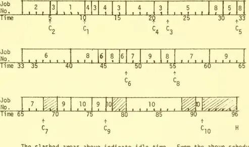
Figure 6 illustrates several steps in the solution procedure. The lower curve shown, £(z,T'), was used to find the initial level z* = 12 for detailed search. After this initial level was found the partition T" was used. The transportation tableau at optimum corresponding to £(12,T")

indicated the following preemptive schedule of job/time slot allocations.

Job No, i 2t f 4 3 4 Tt-4 t I 1 I 1 1 t I f Time

T

25 30 '^4

S

Job No. Time 33 35 l—L—l 1 I_l I 1 \ 9 J i_L_L I t 1 t 9 _l t I L

V5

m

65 Job No. _{_I}7_L

#1^

10 10 10 -I L_J t t Time 65 70 75 80 85 90" <>i yy,^A'y,<^A 96 H

7

^9 ₁₀

The slashed areas above indicate idle time. From the above schedule

a good non-preemptive schedule (tt. = 2-1-4-3-5-6-8-7-9-10) was obtained by sequencing in order of completion times for the transportation tableau

-41

An

adjacent pairwise interchanges in tt. were then evaluated

yielding an improved solution -n^ = _{2-1-3-4-5-6-8-7-9-10 with g(12,Trg)} =

2566. Detailed search of the overtime level z = 12 revealed that ttp, was

b

optimal for this level.

Overtime levels less than z = 12 were then explored and quickly eliminated. The first solution generated for z = 13 was tt. =

2-1-3-4-5-6-8-9-7-10 which yielded the improved cost g(13,TTj,) = 2562.

Detailed search yielded further improvement g(13,iTp,) = 2546 with ttj, = -n^.

This solution also dominated all other z levels greater than 13 and is therefore optimal

.

Note that in this example the lower bounding curve £(z,T') and £(z,T") achieve their minima at the same point. Note also the solution

(12,TT.) constructed from the transportation tableau (after 7 seconds) proved to be very close to optimum.

The computation time (32 sec.) was subdivided as follows:

- _{compute ^(z.T')}

: 1 second

- _{compute 2.(z.T"): 27 seconds}

- _{detailed search of all z levels: 3 seconds}

- _{other operations:}

1 second

The computation of £(z,T") requires about 85 percent of the total time. As indicated in 4.5.4 the computational efficiency depends on the time partitioning: a finer time division gives stronger bounds, but requires to solve transportation problems of higher dimensions. We were

-42-T" by T'" (t'" = _0, t'.'^ = x'." + 2). More complete computational results and a discussion of refinements of the above algorithm are given in [6 ],

u

(2,n)

-43-S^'

1

1

tSi>Z

V

1

y^lSZt

250O

--ZH-00

2M79

ztj6g -ri'tfeH '*i'wr6

^<a(z,T")

2v?9

I I

^iS9

^35

2. _^f^7 C:?,r';

t^oo

.-_, 1-9 10

n

12 13 14 15 16

.44-Concluding Remarks

This paper has formulated the one machine job shop scheduling

problem with variable capacity. A bounding structure has been proposed

which appears to provide considerable insight into the structure of the

optimal solution as well as bounding its cost.

Among the issues which appear fruitful for future research, the following

seem particularly important.

1. Extension of the bounding scheme to more complex aggregate

costs and constraints. In principle, this is straightforward. If the cost and constraint structure of the problem were linear, for example, a

lower bounding problem is formulated with the given aggregate costs and constraints plus the transportation formulation for the detailed level.

The optimal solution to this lower bounding (linear programming) problem

would then be used as a starting point for local search just as the minimum of £(z,T), and a corresponding non-preemptive schedule, were used

in the algorithm above. This procedure would very likely lead to an excellent solution, though bounding of all capacity plans would no doubt be prohibitively expensive in this more general environment where a

single dimension representation of overtime (total overtime) is no longer possible.

2. Extensions and refinements of the algorithm. Cases of interest include: (a) non-simultaneous job arrivals; (b) inclusion of Shwimer's theorem A (generalized) in the detailed search algorithm; (c) inclusion of the slope bounding relations introduced in 4.6.3 (d) more complex

-45-aggregate models as discussed above; and (e) general pruning and testing of the algorithm.

3. Evaluation of alternative heuristics likely to be imple-mentable in more realistic environments. Heuristics of concern are:

(a) methods for determining a good capacity plan; (b) dispatching heuristics; and (c) coordination schemes for iteratively determining

a combined capacity and scheduling plan. The central issue here is to provide normative insight into the resolution of the aggregate-detailed

cost trade-off problem. The extent to which one might be able to extrap-olate such one machine results to more general environments is, of course,, a moot question requiring more complete tests by empirical and simulation studies.

4. Finally, it would be interesting to explore the possibility of extending the transportation bounding scheme to several machines

-46-Appendix I

Proposition (P4): Let r. = 0, j = l,...,n. Then the SPT rule minimizes

F for any given capacity plan.

Proof: Suppose we know the optimal schedule S with respect to F and suppose

that this schedule is not the SPT schedule. By (PI) and (P2) we may assume

S is non-preemptive without inserted idle time. My(T)

S S'

Then: there are adjacent jobs k,Jl such that k<il (k precedes £) and t. > t^^.

Interchanging k and a gives completion times C/ and C' for jobs k and f

in a new schedule called S', and

C^ <_ C^ because t^^^ < t|^ and y{i) is non-decreasing;

^k

^i-Thus C' + C; < C. + Co. But C. = C. -Vj ?^ k,il. Then Z CI < E C. and

K Ji

-

K )t J J _jeN '^

jeN J therefore f'

_^

F. Continuing with pairwise interchanges one may thus

-47-BIBLIOGRAPHY

Buffa, E. S. and Taubert, W. H. Production-Inventory Systems: Planning and Control. Richard D. Irwin, Inc., 1972.

Conway, R. W., W. L. Maxwell and L. W. Miller, Theory of Scheduling,

Addison Wesley (Reading, Mass., 1967).

Dantzig, G. B., Linear Programming and Extensions, Princeton

University Press, 1966.

Elmaghraby, S. E., "The One Machine Sequencing Problem with Delay Costs," Journal of Industrial Engineering, Vol. XIX, No. 2 (February

1968), pp. 105-108.

Emmons, H. , "One-Machine Sequencing to Minimize Certain Functions

of Job Tardiness," Operations Research, Vol. 17, No. 4 (July- August

1969), pp. 701-715.

Gelders, L. and P. R. Kleindorfer, "Coordinating Aggregate and Detailed Scheduling in the One-Machine Job Shop: II - Computation and Structure," unpublished working paper, Sloan School of

Management, MIT, May 1972.

Green, R. S., "Heuristic Coupling of Aggregate and Detail Models in Factory Scheduling," unpublished Ph.D. thesis, Sloan School of Management, MIT (February 1971).

Hadley, G., Linear Programming, Addison-Wesley, 1963.

Held, M. and R. M. Karp, "A Dynamic Programming Approach to Sequencing Problems, " _{Journal of the Society for} Industrial and Applied

Mathematics, Vol. 10, No. 1 (March 1962), pp. 196-210.

Jones, C. H., "Parametric Production Planning," Management Science,

Vol. 13, No. 11 (July 1967), pp. 843-866.

McNaughton, R., "Scheduling with Deadlines and Loss Functions,"

Management Science, Vol. 6, No. 1 (September 1959), pp. 1-12.

Newson, E.P., "Lot Size Scheduling to Finite Capacity," unpublished Ph.D. thesis, Sloan School of Management, MIT (August 1971).

Schild, A. and I. J. Fredman, "On Scheduling Tasks with Associated Linear Loss Function," Management Science, Vol. 7, No. 3 (April

-48-[14]

____^

^."Scheduling

Tasks with Deadlines and

Non-Linear Loss Functions," Management Science, Vol. 9, No. 1

(September 1962), pp. 73-81.

[15] Shwimer, J., "On the'N-job, One-Machine, Sequence-Independent^ Problem with Tardiness Penalties: A Branch and Bound Approach, Management Science. Vol. 18, No. 6 (February 1972), pp. B301-B313.

[16] , "Interaction between Aggregate and Detailed Scheduling

in a Job Shop," unpublished Ph.D. thesis, Sloan School of Management, MIT (June 1972).

[17] SrinivasBn, V., "An Operator Theory of Parametric Programming for the Transportation Problem (I)," Management Science Report #236, GSIA

(Carnegie-Mellon University, March 1971).

[18] , "An Operator Theory of Parametric Programming for the

Transportation Problem (II)," Management Science Report #242, GSIA (Carnegie-Mellon University, April 1971).

[19]

_{___^}

, "A Hybrid Algorithm for the One-Machine Sequencing

Problem to Minimize Total Tardiness," Management Science Report #225, GSIA (Carnegie-Mellon University, November, 1970).

[20] Taubert, W. H., "A Computer Search Solution of the Aggregate Scheduling Problem," Management Science, Vol. 14, No. 6 (February

It.