Hybrid MIMD/SIMD High Order DGTD Solver for the Numerical Modeling of Light/Matter Interaction on the Nanoscale

HAL Id: hal-01253158

https://hal.inria.fr/hal-01253158

Submitted on 8 Jan 2016

HAL is a multi-disciplinary open access

archive for the deposit and dissemination of

sci-entific research documents, whether they are

pub-lished or not. The documents may come from

teaching and research institutions in France or

abroad, or from public or private research centers.

L’archive ouverte pluridisciplinaire HAL, est

destinée au dépôt et à la diffusion de documents

scientifiques de niveau recherche, publiés ou non,

émanant des établissements d’enseignement et de

recherche français ou étrangers, des laboratoires

publics ou privés.

Hybrid MIMD/SIMD High Order DGTD Solver for the

Numerical Modeling of Light/Matter Interaction on the

Nanoscale

Stéphane Lanteri, Raphaël Léger, Claire Scheid, Jonathan Viquerat, Tristan

Cabel, Gabriel Hautreux

To cite this version:

Stéphane Lanteri, Raphaël Léger, Claire Scheid, Jonathan Viquerat, Tristan Cabel, et al.. Hybrid

MIMD/SIMD High Order DGTD Solver for the Numerical Modeling of Light/Matter Interaction on

the Nanoscale. France. PRACE, 2015. �hal-01253158�

Partnership for Advanced Computing in Europe

Hybrid MIMD/SIMD High Order DGTD Solver for

the Numerical Modeling of Light/Matter Interaction on the Nanoscale

S. Lanteri

*, R. Léger

, C. Scheid

and J. Viquerat

T. Cabel

and G. Hautreux

a

INRIA Sophia Antipolis – Méditerannée research center, France

b

CINES, Montpellier, France

Abstract

This paper is concerned with the development of a scalable high order finite element type solver for the numerical modeling of light interaction with nanometer scale structures. From the mathematical modeling point of view, one has to deal with the differential system of Maxwell equations in the time domain, coupled to an appropriate differential model of the behavior of the underlying material (which can be a dielectric and/or a metal) at optical frequencies. For the numerical solution of the resulting system of differential equations, we have designed a high order DGTD (Discontinuous Galerkin Time-Domain) solver that has been adapted to hybrid MIMD/SIMD computing. Here we discuss about this later aspect and report on preliminary performance results on the Curie system of the PRACE research infrastructure.

1. Scientific and technological context

Nanostructuring of materials has opened up a number of new possibilities for manipulating and enhancing light-matter interactions, thereby improving fundamental device properties. Low-dimensional semiconductors, like quantum dots, enable one to catch the electrons and control the electronic properties of a material, while photonic crystal structures allow synthesizing the electromagnetic properties. These technologies may, e.g., be employed to make smaller and better lasers, sources that generate only one photon at a time for applications in quantum information technology, or miniature sensors with high sensitivity. The incorporation of metallic structures into the medium adds further possibilities for manipulating the propagation of electromagnetic waves. In particular, this allows subwavelength localization of the electromagnetic field and, by subwavelength structuring of the material, novel effects like negative refraction, e.g. enabling super lenses, may be realized. Nanophotonics is the field of science and technology aimed at establishing and using the peculiar properties of light and light-matter interaction in various nanostructures. Nanophotonics includes all the phenomena that are used in optical sciences for the development of optical devices. Therefore, nanophotonics finds numerous applications such as in optical microscopy, the design of optical switches and electromagnetic chips circuits, transistor filaments, etc. Because of its numerous scientific and technological applications (e.g. in relation to telecommunication, energy production and biomedicine), nanophotonics represents an active field of research increasingly relying on numerical modeling beside experimental studies.

* Corresponding author. E-mail address: Stephane.Lanteri@inria.fr 1

Plasmonics [1] is a related field to nanophotonics. Metalic nanostructures whose optical scattering is dominated by the response of the conduction electrons are considered as plasmomic media. If the structure presents an interface with e.g. a dielectric with a positive permittivity, collective oscillations of surface electrons create surface-plasmons-polaritons (SPPs) that propagate along the interface. SPPs are guided along metal-dielectric interfaces much in the same way light can be guided by an optical fiber, with the unique characteristic of subwavelength-scale confinement perpendicular to the interface. Nanofabricated systems that exploit SPPs offer fascinating opportunities for crafting and controlling the propagation of light in matter. In particular, SPPs can be used to channel light efficiently into nanometer-scale volumes, leading to direct modification of mode dispersion properties (substantially shrinking the wavelength of light and the speed of light pulses for example), as well as huge field enhancements suitable for enabling strong interactions with nonlinear materials. The resulting enhanced sensitivity of light to external parameters (for example, an applied electric field or the dielectric constant of an adsorbed molecular layer) shows great promise for applications in sensing and switching. In particular, very promising applications are foreseen in the medical domain [2]-[3].

2. Mathematical and numerical modeling

In the computational nanophotonics literature, a large number of studies are devoted to Finite Difference Time-Domain (FDTD) type discretization methods based on Yee’s scheme [4]-[5]. As a matter of fact, the FDTD method is a widely used approach for solving the systems of partial differential equations modeling nanophotonic applications. In this method, the whole computational domain is discretized using a structured (Cartesian) grid. However, in spite of its flexibility and second-order accuracy in a homogeneous medium, the Yee scheme suffers from serious accuracy degradation when used to model curved objects or when treating material interfaces. During the last twenty years, numerical methods formulated on unstructured meshes have drawn a lot of attention in computational electromagnetics with the aim of dealing with irregularly shaped structures and heterogeneous media. In particular, the discontinuous Galerkin time-domain (DGTD) method has progressively emerged as a viable alternative to well established finite-difference time-domain (FDTD) and finite-element time-domain (FETD) methods for the numerical simulation of electromagnetic wave propagation problems in the time-domain. In this work, we are concerned with the design of such a DGTD method for nanophotonics.

2.1 Generalities about the DGTD method

The DGTD method can be considered as a finite element method where the continuity constraint at an element interface is released. While it keeps almost all the advantages of the finite element method (large spectrum of applications, complex geometries, etc.), the DGTD method has other nice properties, which explain the renewed interest it gains in various domains in scientific computing:

 It is naturally adapted to a high order approximation of the unknown field. Moreover, one may increase the degree of the approximation in the whole mesh as easily as for spectral methods but, with a DGTD method, this can also be done locally i.e. at the mesh cell level. In most cases, the approximation relies on a polynomial interpolation method but the method also offers the flexibility of applying local approximation strategies that best fit to the intrinsic features of the modeled physical phenomena.

 _{When the discretization in space is coupled to an explicit time integration method, the DG method} leads to a block diagonal mass matrix independently of the form of the local approximation (e.g the type of polynomial interpolation). This is a striking difference with classical, continuous FETD formulations. Moreover, the mass matrix is diagonal if an orthogonal basis is chosen.

 It easily handles complex meshes. The grid may be a classical conforming finite element mesh, a non-conforming one or even a hybrid mesh made of various elements (tetrahedra, prisms, hexahedra, etc.). The DGTD method has been proven to work well with highly locally refined meshes. This property makes the DGTD method more suitable to the design of a hp-adaptive solution strategy (i.e. where the characteristic mesh size h and the interpolation degree p changes locally wherever it is needed).

 _{It is flexible with regards to the choice of the time stepping scheme. One may combine the} discontinuous Galerkin spatial discretization with any global or local explicit time integration scheme, or even implicit, provided the resulting scheme is stable.

 It is naturally adapted to parallel computing. As long as an explicit time integration scheme is used, 2

the DGTD method is easily parallelized. Moreover, the compact nature of method is in favor of high computation to communication ratio especially when the interpolation order is increased.

As in a classical finite element framework, a discontinuous Galerkin formulation relies on a weak form of the continuous problem at hand. However, due to the discontinuity of the global approximation, this variational formulation has to be defined at the element level. Then, a degree of freedom in the design of a discontinuous Galerkin scheme stems from the approximation of the boundary integral term resulting from the application of an integration by parts to the element-wise variational form. In the spirit of finite volume methods, the approximation of this boundary integral term calls for a numerical flux function, which can be based on either a centered scheme or an upwind scheme, or a blend of these two schemes. In the early 2000’s, DGTD methods for time-domain electromagnetics have been first proposed by mainly three groups of researchers. One of the most significant contributions is due to Hesthaven and Warburton [6] in the form of a high order nodal DGTD method formulated on unstructured simplicial meshes. The proposed formulation is based on an upwind numerical flux, nodal basis expansions on a triangle (2D case) and a tetrahedron (3D case) and a Runge-Kutta time stepping scheme. In [7], Kakbian et al. describe a rather similar approach. More precisely, the authors develop a parallel, unstructured, high order DGTD method based on simple monomial polynomials for spatial discretization, an upwind numerical flux and a fourth-order Runge-Kutta scheme for time marching. The method has been implemented with hexahedral and tetrahedral meshes. Finally, a high order nodal DGTD method formulated on unstructured simplicial meshes has also been proposed in the same time frame by Fezoui et al. [8]. However, contrary to the DGTD methods discussed in [6] and [7], the method proposed in [8] is non-dissipative thanks to a combination of a centered numerical flux with a second-order leapfrog time stepping scheme.

2.2 A non-dissipative DGDT method for nanophotonics/plasmonics

Numerical modeling of electromagnetic wave propagation in interaction with metallic nanostructures at optical frequencies requires solving the system of Maxwell equations coupled to appropriate models of physical dispersion in the metal. In general, the Drude and Drude-Lorentz models are adopted although there are practical situations for which these models can fail to describe correctly the behavior of some materials (e.g. transition metals [9]-[10] and graphene [11]). Furthermore at some scales, non-local effects starts to play an important role [12]. With all their features (as described above), DGTD methods seem to be well suited to the numerical simulation of complex time-domain electromagnetic wave propagation problems. As a matter of fact, the DGTD method for solving the time domain Maxwell equations is increasingly adopted by several physics communities. Concerning nanophotonics, unstructured mesh based DGTD methods have been developed and have demonstrated their potentialities for being considered as viable alternatives to the FDTD method [13]-[14]-[15]-[16]-[17]-[18]-[19]. Noteworthy, all these studies adopt a diffusive DGTD formulation based on upwind numerical fluxes.

Towards the general aim of being able to consider concrete physical situations relevant to nanophotonics, one has to take into account in the numerical treatment, a better description of the propagation of waves in realistic media. The physical phenomenon that one has to consider in the first instance here is dispersion. In the presence of an electric field the medium cannot react instantaneously and thus presents an electric polarization of the molecules or electrons that itself influences the electric displacement. In the case of a linear homogeneous isotropic media, there is a linear relation between the applied electric field and the polarization. However, above some range of frequencies (depending on the considered material), the dispersion phenomenon cannot be neglected and the relation between the polarization and the applied electric field becomes complex. In practice, this is modeled by a frequency dependent complex permittivity. Several such models for the characterization of the permittivity exist; they are established by considering the equation of motion of the electrons in the medium and making some simplifications. There are mainly two ways of handling the frequency dependent permittivity in the framework of time-domain simulations, both starting from models defined in the frequency time-domain. A first approach is to introduce the polarization vector as an unknown field through an auxiliary differential equation, which is derived from the original model in the frequency domain by means of an inverse Fourier transform. This is called the Direct Method or Auxiliary Differential Equation (ADE) formulation. Let us note that while the new equations can be easily added to any time-domain Maxwell solver, the resulting set of differential equations is tied to the particular choice of dispersive model and will never act as a black box able to deal with other models. In the second approach, the electric field displacement is computed from the electric

field through a time convolution integral and a given expression of the permittivity which formulation can be changed independently of the rest of the solver. This is called the Recursive Convolution Method (RCM). We have recently adapted the DGTD method initially introduced in [8] to deal with various dispersion models. An ADE formulation has been adopted. We first considered the case of Drude and Drude-Lorentz models and, further extend the proposed ADE-based DGTD method to be able to deal with a generalized dispersion model in which we make use of a Padé approximant to fit an experimental permittivity function. In this paper, we focus on the case of the Drude model. The latter is associated to a particularly simple theory that successfully accounts for the optical and thermal properties of some metals. In this model, the metal is considered as a static lattice of positive ions immersed in a free electrons gas. Those electrons are considered to be the valence electrons of each metallic atom that got delocalized when put into contact with the potential produced by the rest of the lattice atoms. The DGTD method proposed in

[20] relies on a compact stencil high order interpolation of the electromagnetic field components within each cell of an unstructured tetrahedral mesh. This piecewise polynomial numerical approximation is allowed to be discontinuous from one mesh cell to another, and the consistency of the global approximation is obtained thanks to the definition of appropriate numerical traces of the fields on a face shared by two neighboring cells. Time integration is achieved using an explicit scheme and no global mass matrix inversion is required to advance the solution at each time step. As a result, this DGTD solver is particularly well adapted to parallel computing. The resulting ADE-based DGTD method is detailed in [20] and is part of a larger initiative aiming at the development of a software suite dedicated to nanophotonics/nanoplasmonics.

3. DGTD code workflow and parallelization

The DGTD method outlined in section 2 for solving the system of 3d time-domain Maxwell equations coupled to a dispersion model for a metal such as the Drude model (we refer below to the resulting coupled system as the Maxwell-Drude system) has been implemented in simulation software programmed in Fortran 95. The DGTD method is formulated on an unstructured tetrahedral mesh. Within each element of the mesh, the components of the electromagnetic field are approximated by a arbitrary high order nodal polynomial interpolation method. The unknowns of the problem are 3-component vectors that depend on the spatial coordinate vector x = (x,y,z) and the time t: the electric field E, the magnetic field H and the electric polarization vector P. At the discrete level, the objective is to solve the Maxwell-Drude system for Eh, Hh and Ph (here h denotes the spatial discretization parameter) at a set of nodal points

associated to Lagrange type basis functions defined on simplicial elements. Note that, contrary to the FDTD method, the unknown components of these three vectors are collocated in the spatial grid. As it is usually done in standard finite element approaches, elemental terms appearing in the variational formulation of the problem are evaluated and stored on a reference tetrahedron and then transformed to the physical tetrahedra using a bijective affine map (the underlying spatial grid is assumed to rely on affine tetrahedra only). The spatial interpolation order within each element of the mesh is arbitrary (but in the current implementation of the DGTD solver the spatial interpolation order is uniform i.e. is the same for all the tetrahedra of the mesh). The local (i.e. element-wise) number of degrees of freedom is equal to 9np where np is the number of basis functions for a pth order interpolation. For p = 1,2,3,4,5 the number np

is respectively equal to (p+1)(p+2)(p+3)/6.

From the algorithmic point of view, the DGTD method mainly involves matrix-vector product operations that are performed at the tetrahedron level, involving a set of local matrices corresponding to integral terms of the weak formulation of the method. Indeed, two types of integral terms latter appear in the weak formulation:

 Volume integral terms i.e. whose support is a tetrahedron: one of this term leads to the definition of a local mass matrix, while the other term corresponds to a local pseudo-stiffness matrix. These are square matrices.

 Surface (or boundary) integral terms i.e. whose support is the boundary of a tetrahedron: this term couples the local solution computed in a tetrahedron to its face-wise neighbors. This integral term leads to the definition of the so-called local interface matrix. These are square matrices if the interpolation order is the same for each tetrahedron (and thus, each face of a tetrahedron).

The sizes of these local matrices, which are dense matrices, depend on the interpolation order of the components of the physical fields in a tetrahedron. For instance, the mass and pseudo-stiffness matrices are of size np x np.

The coarse grain parallelization of the DGTD code is based on a SPMD approach. It relies on a partitioning of the underlying tetrahedral mesh (this step is performed using a separate toolkit specifically designed for that purpose and making use of existing graph partitioning tools such as MeTiS or PT-Scotch). Then, in this SPMD version, each submesh of the partition is treated by one single MPI process.

The resulting DGTD simulation software is structured into 3 phases (see Fig. 1):

1. A pre-preprocessing phase, which essentially consists in operations, related to the definition of the problem under consideration (reading of the computational mesh and simulation parameters, construction of geometrical entities related data structures, definition of the initial distribution of the electromagnetic field and source terms, etc.). In this pre-processing phase, communication lists – which are the index lists of faces that connect two neighboring submeshes - are built. 2. The main time-stepping loop, which represents the core processing part of the unsteady

simulation. The selected time-stepping scheme is fully explicit so there is no matrix inversion step (or linear system solve), because of the discontinuous nature of the approximation in space (i.e. the discontinuous Galerkin method leads to block diagonal mass matrices).

3. A post-processing phase, which is concerned with all the operations, related to the treatment of the numerical solution in view of further visualization and other operations.

The relative proportion in terms of CPU time of these 3 steps depends on the number of iterations of the time advancing procedure. Typically in the initial setting of the problem, the time-stepping loop takes about 90% of the total time whereas the pre and post processing phases share the remaining 10%.

Fig.1: Workflow of the DGTD simulation.

The main time stepping loop essentially consists in four phases:

1. Update the electric field Eh at time station (n+1)Dt form the known fields Eh at time station nDt and

magnetic field Hh at time station (n+1/2)Dt.

2. Update the electric polarization vector Ph at time station (n+1)Dt form the known polarization

vector Ph at time station nDt and field electric Eh at time stations nDt and (n+1)Dt.

3. Update the electric field Hh at time station (n+3/2)Dt form the known fields magnetic field Hh at

time station (n+1/2)Dt and Eh at time station (n+1)Dt.

4. Perform auxiliary calculations: compute the DFT (discrete Fourier transform) of the Eh and Hh fields

on the fly, update the imposed incident field (for test problems for which this field is required), 5

update the imposed source current density (for test problems for which this current density is required) and perform some edition and I/O operations of intermediate results.

The first and third phases correspond to two separate routines whose structures are very similar:

1. Definition of the fictious fields associated to the boundary conditions on the physical boundaries faces (purely local operation).

2. Definition of the fictious fields associated to the artificial boundary faces (requires point-to-point communication operations).

3. Contribution of the boundary integral over the face of a tetrahedron to the flux balance of this tetrahedron, for each face of the tetrahedron.

4. Contribution of the volume integral over a tetrahedron for the curl operator to the flux balance of this tetrahedron.

5. Update of the field in a tetrahedron using the flux balance of this tetrahedron.

Steps 1 and 2 allow gathering the data necessary to perform step 3 in a purely local way. Steps 4 and 5 are purely local i.e. do not require to access the fields of neighboring tetrahedra of a given tetrahedron. Step 2 involves matrix-vector product operations with the interface matrix, while in step 4 matrix-vector product operations are performed with the mass and pseudo-stiffness matrices. Note that step 3, 4, 5 are based on a loop through the cell of the local submesh.

Because of the use of an explicit time stepping method and the local nature of the formulation, the time advancing of the components of the Eh and Hh fields at the degrees of freedom of one tetrahedron only

depends of the local values of these fields, and on the field values at the degrees of freedom localized on the faces shared by the tetrahedron and its direct neighboring tetrahedra. Therefore, at each iteration of the time stepping phase, it is necessary to send and receive values of the components of the Eh and Hh

fields for the degrees of freedom of the set of faces lying on an interface (triangular surface) between neighboring submeshes. For both fields (i.e. once in each of the ELECTR and MAGNET routines), this requires point-to-point communication operations between 2 adjacent submeshes. The size of the MPI buffers depend on the number of degrees of freedom on one face and the length of the communication list, i.e. the number of facets that connect submeshes to each other. Note that we are using an updating scheme based on non-blocking operations (both interface updating strategies will be available and the selection will be possible through a single flag set in the pre-processing phase). Note that the space-time evolution of the electric polarization in the Maxwell-Drude equations is modeled by a system of ordinary differential equations. Therefore, the time advancing of Ph at the degrees of freedom of one tetrahedron only depends

of the local values of Ph. Moreover, at each time step, if required, the discrete electromagnetic energy is

computed in every submesh and globally reduced through a global communication operation.

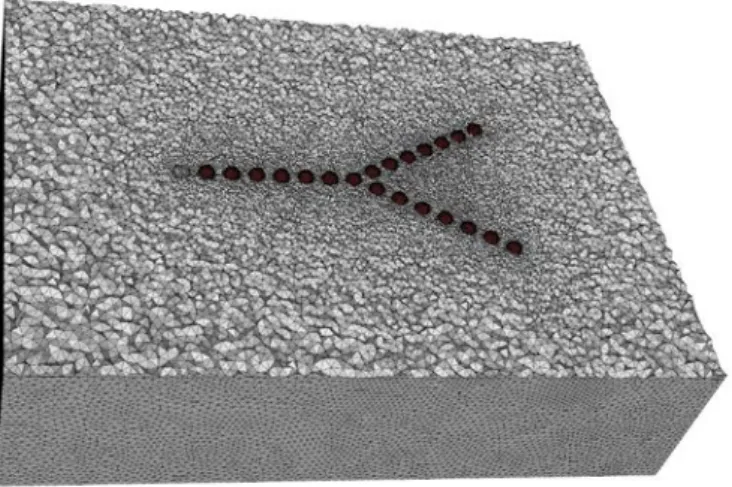
4. Scalability evaluation

We limited ourselves to a parallel performance evaluation in terms of strong scalability analysis. For that purpose, we selected a use case typical of optical guiding applications. A Y-shaped waveguide is considered which consists in nanosphere embedded in vacuum. The computational domain is shown of Fig. 2 below. The constructed tetrahedral mesh consists of 520,704 vertices and 2,988,103 elements. The high order discontinuous finite element method designed for the solution of the system of time-domain Maxwell equations coupled to a Drude model for the dispersion of noble metals at optical frequencies is formulated on a tetrahedral mesh. Within each element (tetrahedron) of the mesh, the components of the electric and magnetic field, as well as the component of the electric polarization, are approximated by a nodal (Lagrange type) interpolation method. The unknowns of the problem are thus given by the values of these physical quantities at the nodes of the polynomial interpolation. For instance, for a linear (i.e. P1)

interpolation of the fields, the number of DoFs (Degrees of Freedoms) within a tetrahedron is 6x4 if the element is located in vacuum, and 9x4 if the element is located in the metallic structure. For a quadratic (i.e. P2) interpolation, the corresponding figures are 6x10 and 9x10, and so on for higher interpolation

degrees. Then the global number of DoFs is the sum of these figures of the elements of the given mesh.

Fig.2: View of the computational domain for the Y-shaped waveguide.

Fig. 3: Contour lines of the amplitude of the discrete Fourier transform of the electric field.

The strong scalability analysis has been conducted on the thin nodes of the Curie system. Each run has been made considering 8 OpenMP threads per socket and 2 sockets per node. Plots of the parallel speedup of the DGTD solver with P2 (top), P3 (middle) and P4 (bottom) interpolation are shown on Fig. 4. The maximum number of cores that has been exploited is 8192 for a simulation based on the DGTD-P4 method.

A quasi-ideal scaling is obtained up to 1024 cores. Achieving a better parallel speedup for a number of cores greater than 1024 would probably require a finer tetrahedral mesh (with several million mesh vertices). Simulation times as well as speedup values are summarized in Tab. 1-3 below.

Fig.4: Strong scalability analysis of the DGTD solver with P2 (top), P3 (middle) and P4 (bottom) interpolation.

Number of cores Wall clock time Speed-up vs. the

first one Number of Nodes Number of process (MPI+OpenMP)

128 4066 sec 1.00 8 128

256 1972 sec 2.00 16 256

512 952 sec 4.05 32 512

1024 462 sec 8.40 64 1024

Tab. 1: Strong scaling of the DGTD solver with P2 interpolation (on each node, we spawn 2 MPI process and 8

OpenMP threads per MPI process).

Number of cores Wall clock time Speed-up vs. the

first one Number of Nodes Number of process (MPI+OpenMP)

512 2580 sec 1.00 32 512

1024 1271 sec 2.00 64 1024

2048 646 sec 4.00 128 2048

Tab. 2: Strong scaling of the DGTD solver with P3 interpolation (on each node, we spawn 2 MPI process and 8 OpenMP

threads per MPI process).

Number of cores Wall clock time Speed-up vs. the

first one Number of Nodes Number of process (MPI+OpenMP)

2048 1714 sec 1.00 128 256

4096 897 sec 1.90 256 512

8192 529 sec 3.25 512 1024

Tab. 3: Strong scaling of the DGTD solver with P4 interpolation (on each node, we spawn 2 MPI process and 8

OpenMP threads per MPI process).

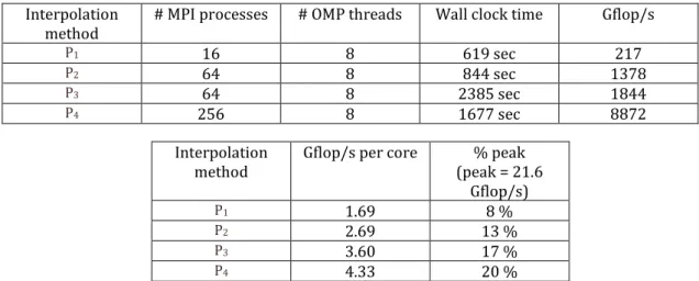
Finally, the computational performances of the DGTD solver for the considered problem size are reported in Tab. 4 below. As expected, the performances increase with the interpolation degree in the DGTD method. Indeed, when the interpolation degree is raised, the amount of local (i.e. at the element level) operations increases accordingly (recall that these local operations take the form of dense matrix/matrix and matrix/vector products).

Interpolation

method # MPI processes # OMP threads Wall clock time Gflop/s

P1 16 8 619 sec 217

P2 64 8 844 sec 1378

P3 64 8 2385 sec 1844

P4 256 8 1677 sec 8872

Interpolation

method Gflop/s per core (peak = 21.6 % peak Gflop/s)

P1 1.69 8 %

P2 2.69 13 %

P3 3.60 17 %

P4 4.33 20 %

Tab. 4: Computational performances of the DGTD solver.

References

[1] S. Maier. Plasmonics - Fundamentals and applications. Springer, 2007.

[2] A. Csaki, T. Schneider, J. Wirth, N. Jahr, A. Steinbrück, O. Stranik, F. Garwe, R. Müller and W. Fritzsche.

Molecular plasmonics: light meets molecules at the nanoscale. Phil. Trans. R. Soc. A, 369 (2011) 3483-3496.

[3] Y.B. Zheng, B. Kiraly, P.S. Weiss and T.J. Huang. Molecular plasmonics for biology and nanomedicine. Nanomedicine, 5 (7) (2012) 751-770.

[4] A. Taflove, S. Hagness. Computational electrodynamics: the finite-difference time-domain method - 3rd

ed. Artech House Publishers, 2005.

[5] K.S. Yee. Numerical solution of initial boundary value problems involving Maxwell's equations in isotropic media. IEEE Trans. Antennas and Propagation, 14 (3) (1966) 302-307.

[6] J. Hesthaven, T. Warburton. Nodal high-order methods on unstructured grids. I. Time-domain solution of

Maxwell’s equations. J. Comput. Phys., 181 (1) (2002) 186–221.

[7] V. Kabakian, V. Shankar, W. Hall. Unstructured grid-based discontinuous Galerkin method for broadband

electromagnetic simulations. J. Sci. Comput., 20 (3) (2004) 405–431.

[8] L. Fezoui, S. Lanteri, S. Lohrengel, S. Piperno. Convergence and stability of a discontinuous Galerkin

time-domain method for the 3D heterogeneous Maxwell equations on unstructured meshes. ESAIM: Math. Model.

Numer. Anal., 39 (6) (2005) 1149–1176.

[9] R. Ulbricht, E. Hendry, J. Shan, T. Heinz, M. Bonn. Carrier dynamics in semiconductors studied with

time-resolved terahertz spectroscopy. Rev. Mod. Phys., 83 (2) (2011) 543–586.

[10] C. Wolff, R. Rodrguez-Oliveros, K. Busch. Simple magneto-optic transition metal models for

time-domain simulations. Optics Express 21 (10) (2013) 12022–12037.

[11] F. J. G. de Abajo. Graphene nanophotonics. Science - Applied Phys., 339 (2013) 917–918.

[12] A. Moreau, C. Ciraci, D. Smith. Impact of nonlocal response on metallo-dielectric multilayers and optical patch antennas. Phys. Rev. B 87 (045401-1–045401-11) (2013) 6795–6820.

[13] R. Diehl, K. Busch, J. Niegemann. Comparison of low-storage Runge-Kutta schemes for discontinuous

Galerkin time-domain simulations of Maxwell’s equations. J. Comp. Theor. Nanosc., 7 (2010) 1572.

[14] K. Stannigel, M. Koenig, J. Niegemann, K. Busch. Discontinuous Galerkin time-domain computations of

metallic nanostructures. Optics Express, 17 (2009) 14934–14947.

[15] B. Zhu, J. Chen, W. Zhong, Q. Liu. Analysis of photonic crystals using the hybrid

finite-element/finite-difference time domain technique based on the discontinuous Galerkin method. Int. J. Numer. Meth. Eng. 92

(5) (2012) 495–506.

[16] J. Niegemann, M. König, K. Stannigel, K. Busch. Higher-order time- domain methods for the analysis of

nano-photonic systems. Photonics Nanostruct., 7 (2009) 2–11.

[17] K. Busch, M. König, J. Niegemann. Discontinuous Galerkin methods in nanophotonics. Laser and Photonics Reviews 5 (2011) 1–37.

[18] C. Matysseka, J. Niegemann, W. Hergertb, K. Busch. Computing electron energy loss spectra with the

Discontinuous Galerkin Time-Domain method. Photonics Nanostruct., 9 (4) (2011) 367–373.

[19] J. Niegemann, R. Diehl, K. Busch. Efficient low-storage Runge-Kutta schemes with optimized stability

regions. J. Comput. Phys., 231 (2) (2012) 364–372.

[20] J. Viquerat, S. Lanteri, C. Scheid. Theoretical and numerical analysis of local dispersion models coupled

to a discontinuous Galerkin time-domain method for Maxwell’s equations. INRIA Research Report RR-8298

(2013).

Acknowledgements

This work was financially supported by the PRACE project funded in part by the EUs 7th Framework Programme (FP7/2007-2013) under grant agreement no. RI-312763.