Agricultural risk, remittances and climate change in rural Africa

(1)

HAL Id: tel-01724418

https://tel.archives-ouvertes.fr/tel-01724418

Submitted on 6 Mar 2018

HAL is a multi-disciplinary open access

archive for the deposit and dissemination of sci-entific research documents, whether they are pub-lished or not. The documents may come from teaching and research institutions in France or abroad, or from public or private research centers.

L’archive ouverte pluridisciplinaire HAL, est destinée au dépôt et à la diffusion de documents scientifiques de niveau recherche, publiés ou non, émanant des établissements d’enseignement et de recherche français ou étrangers, des laboratoires publics ou privés.

Agricultural risk, remittances and climate change in

rural Africa

Stefanija Veljanoska

To cite this version:

Stefanija Veljanoska. Agricultural risk, remittances and climate change in rural Africa. Economics and Finance. Université Panthéon-Sorbonne - Paris I, 2016. English. �NNT : 2016PA01E057�. �tel-01724418�

(2)

Université Paris 1 Panthéon-Sorbonne

et

Paris School of Economics

Agricultural risk, remittances and climate change in

rural Africa

Stefanija Veljanoska

Thèse présentée et soutenue publiquement

à l’Université Paris 1 Panthéon-Sorbonne le 9 décembre 2016 en vue de l’obtention du grade de

Docteur en sciences économiques

de l’Université Paris 1 Panthéon-Sorbonne et Paris School of Economics

Sous la direction de:

Katrin Millock, Chargée de recherche CNRS, PSE

Jury:

Pascale Combes Motel Professeur, Université d’Auvergne, CERDI

Margherita Comola Maître de Conférences, Université Paris 1 Panthéon-Sorbonne, PSE Salvatore Di Falco Professeur, Université de Genève

(3)

L’université Paris I Panthéon-Sorbonne n’entend donner aucune approbation ni

improbation aux opinions émises dans cette thèse. Ces opinions doivent être considérées

(4)

(5)

Acknowledgments

First and foremost, I am greatly thankful to Katrin Millock for accepting to be my Ph.D. advisor. I learnt a lot form her during the last four years. I thank her for the precious and continuous advices regarding my research, but also for guiding me in the academic environment. Her careful approach to every stage of my work during this period is of great importance for me. I thank her for being always available, despite her charged schedule, for her kindness, for her support and for all inspiring discussions.

I deeply acknowledge Pascale Combes Motel, Margherita Comola, Salvatore Di Falco and Alberto Zezza for serving on my Ph.D. committee. I thank them for their time and effort in reading and in providing valuable and constructive comments during the pre-defense for the improvement of my work.

I thank Marie-Anne Valfort for her insightful suggestions during my “bilan 12-18”. I thank Viviane Makougni, Elda André, Joel and Loïc Sorel for their numerous advices and help, and for making the MSE a very pleasant place to work. I thank all the members of the Environmental axis, Katheline Schubert, Mireille Chiroleu Assouline, Mouez Fodha, Antoine d’Autume, Hélène Ollivier and Fanny Henriet, for the rewarding seminars and talks. It is a real pleasure to work in and be surrounded by such an environment.

The whole adventure called “writing a Ph.D dissertation” is special because of the oppor-tunity we have to meet extraordinary people. The list is long. Antoine, Vincent, Bertrand, Anastasia, Ezgy, Sebastian, Sandra, Yvan, Mehdi, Elliot, Anna, Francesco, Diana, Victoire, Zaneta, Pierre, Rudy, Margarita, Esther, Djamel, Elsa, Farshad, Nelly, Emanuelle,

(6)

Math-ieu, Anna, Moutaz, Federica, Mabe, Fatma, Nicos, Paolo and Lorenzo thank you for all the discussions and nice moments that we shared during all these years. I thank all the office mates and friends: Lorenzo, Baris, Hamzeh, Mathias, Diane, Yassine, Dmitri, Can, Emna, Pauline, Catharina, Ilya and Masha for their continuous encouragement and for providing means of relaxation all the time. I had the chance to share the apartment with Alessandra, but not only the apartment. We shared friends, Giulia, Joanna, Lenka, Fulvio, Carolina, Emanuelle, Vittorio, Mehmet; we shared recipes, dinners and most of all we shared incredible moments. I thank Julian, Marco and Alexia for contributing to my “flatmate” experience. Thomas had the chance to have three roles, a friend, a colleague and a flatmate. I thank him for all advises and encouragements, especially during these last months. I thank: Hamzeh and Razieh for their kindness, support and all Sunday dinners; Baris for all passionate dis-cussions and advices; Diane for her unconditional help (in all senses) and friendship; Thais and Juliette for the memorable time and talks we had during these four years; Ingrid for interpreting very well her role of “Ph.D. sister”; Anca for being the best conference friend; Anil, Alice, Hélène, Steven, Sanela, Jadran, Chaghaf, Rémi, Lucie, Bojana, Jill, Alice, Igor, Fanny, Sarah, Maria, Nico, Aurélie, Paul-Joseph, Amélie, Jules and Isaure for being so good at saying the right things at the right moment. For ten years we walked side by side with Anil, and then, at some point, Hélène joined us. I am very lucky to be accompanied by them on the journey. I thank Geoffrey for his adaptability, his (in)appropriate jokes and for being such a good listener of complains. I thank the Macedonian team: Elena, Ana, Sofi, Ljupka, Solza, Bisera, Marija, Goce and Jelena, for always being “virtually” there. Your continuous friendship and support has always been a motivation for me.

(7)

A part from the friends that I have already mentioned above, I want to thank Claude, Pascale, Louisette, Quentin and their family for making me discover the French culture, for all the Christmas Eves spent together, for all the warmth and all the support. I thank them for making me feel that I am part of the family. And last, but not the least, I thank my whole family for believing in me. I thank my grandmother for respecting all my decisions and for teaching me to think rationally. I thank my parents for the lifelong support and unconditional love. And, I thank my mother for carefully watching over every single step I made and providing me with advises that helped to build my path.

(8)

List of Tables

1.1 Average remittances in t − 1 . . . 28

1.2 Shocks experienced in the last 12 months . . . 33

2.1 Definition of the diversity indices . . . 42

2.2 Summary statistics of the dependent variables . . . 45

2.3 Estimation results: Beta Coefficients . . . 46

2.4 Definition and descriptive statistics of the explanatory variables on the whole sample and by group of HHs . . . 48

2.5 Descriptive statistics of the count index in 2010/2011 by group of HHs . . . 49

2.6 First Stage estimation . . . 58

2.7 Second stage estimation of number of crops. . . 61

2.8 Second stage estimation of the effect on absolute abundance . . . 62

2.9 Second stage estimation of the effect on relative abundance . . . 63

2.10 Second stage estimation of the effect on relative abundance . . . 64

2.11 Second stage estimation of the effect on riskiness. . . 67

2.12 Second stage estimation of the effect of migration on relative abundance . . 69

(12)

A2 Average crop revenue share . . . 77

3.1 Descriptive statistics of the dependent variable . . . 83

3.2 Descriptive statistics of the dependent variable by group of HHs . . . 85

3.3 Definition and descriptive statistics of the explanatory variables on the whole sample and by group of HHs . . . 86

3.4 Panel Probit estimation on fertilizer use . . . 97

3.5 Panel Tobit estimation on the fertilizer use and intensity . . . 99

3.6 First Stage estimation . . . 101

3.7 IV estimation on organic fertilizer use and its intensity . . . 102

3.8 IV estimation on inorganic fertilizer use and its intensity . . . 103

3.9 Share of households that purchase org. fertilizer . . . 105

3.10 The impact of remittances on livestock . . . 106

4.1 Definition and descriptive statistics . . . 115

4.2 Land acquisition . . . 116

4.3 First stage estimation - Inherited land as instrumental variable . . . 123

4.4 The impact of fragmentation: count measure . . . 126

4.5 The impact of fragmentation: Simpson index . . . 127

4.6 Quantifying the effects . . . 127

4.7 The impact of fragmentation: different soil type . . . 130

4.8 The impact of fragmentation including distance . . . 131

4.9 The impact of fragmentation including temperature . . . 133

(13)

5.1 Summary statistics for the dependent variables. . . 148

5.2 Summary statistics for the explanatory variables . . . 148

5.3 Differences in means depending on the incidence of riots . . . 149

5.4 Impact of the Gini coefficient of water use on the frequency of riots in t and

t + 1 (negative binomial regression) . . . 151

5.5 Impact of the scaled Gini coefficient of water use on the frequency of riots in

t and t + 1 (negative binomial regression) . . . 152

5.6 Impact of the Gini coefficient of water use on the incidence of riots in t and

t + 1 (linear probability estimation) . . . 153

5.7 Impact of the scaled Gini coefficient of water use on the incidence of riots in

t and t + 1 (linear probability estimation) . . . 154

5.8 Summary statistics of the other inequality measures . . . 155

5.9 Impact of the income Gini coefficient (unscaled and scaled) on the frequency

of riots in t and t + 1 (negative binomial regression) . . . 156

5.10 Impact of the income Gini coefficient (unscaled and scaled) on the incidence of riots in t and t + 1 (linear probability estimation) . . . 158

5.11 Impact of the Gini coefficient of land distribution (unscaled and scaled) on the frequency of riots in t and t + 1 (negative binomial regression) . . . 158

5.12 Impact of the Gini coefficient of land distribution (unscaled and scaled) on

the incidence of riots in t and t + 1 (linear probability estimation) . . . 159

5.13 Impact of the different Gini coefficients on the frequency of any conflict events in t and t + 1 (negative binomial regression) . . . 160

(14)

List of Figures

1.1 Time line of rainy and cropping seasons for year t . . . 26

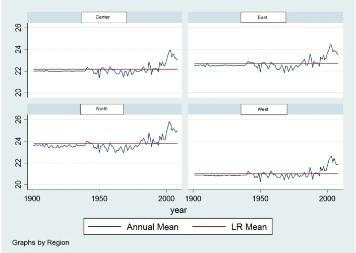
1.2 Rainfall variability in Uganda for the 4 Regions: annual mean and long run

mean Source: Author’s calculation on the CRU TS3.21 dataset . . . 30

1.3 Temperature variability in Uganda for the 4 Regions: annual mean and long run mean Source: Author’s calculation on the CRU TS3.21 dataset . . . 31

1.4 Rainfall deviation by district in the years of the survey from left to right: 2005/2006, 2009/2010, 2010/2011 and 2011/2012 Source: Author’s calculation on the CRU TS3.21 dataset . . . 32

4.1 Distribution of parcels . . . 116

4.2 Rain deviation in absolute terms in the 80 districts . . . 117

4.3 Predicted yield for different levels of rain deviation and number of parcels . . 128

(15)

Chapter 1 Introduction

Risk has a paramount impact on livelihoods in the developing countries. It comes from various sources: climatic, economic, political or individual-specific sources. There are two undisputed facts about Sub-Saharan Africa. The first one is that households’ income is highly volatile and uncertain. The second one is that poverty is commonly present in this part of the world. Uninsured risk can cause shortfalls in income and consumption that can lead households into persistent poverty. Its consequences can be severe for people’s living conditions; it can bring them to a certain minimal acceptable level of income and, without any protection, it can result in hardship.

However, people can take actions to protect themselves against risk. These actions can be diverse as the type of risk/shock faced by households are different. In particular, income variability and losses can be caused by common (aggregate) risk, or individual-specific (id-iosyncratic) risk. Common or aggregate risk is a covariate risk that is faced by all members of a given community or a region. The idiosyncratic risk is specific to a particular individual.

(16)

Households encounter shocks1 _{that include both characteristics, covariate and idiosyncratic.}

When describing the strategies that households use to cope with risk, the frequency, intensity and the persistence of their impact are features to be considered as they can question the efficiency of these strategies [Dercon, 2005].

Formal protection through credit and insurance markets is incomplete or even absent in these countries [Bell,1988,Besley,1995]. Therefore, households have developed sophisticated strategies in order to manage risk. Individual-specific shocks can be smoothed within a community through risk-sharing strategies. Risk-sharing can be considered as an individual consumption smoothing as a result of a membership in a given network or community. If all members of a community are affected by a common shock, then risk cannot be shared. In that case, transfers from outside the community or inter-temporal transfers can be the only possibility that households might have to buffer the shock and smooth consumption. The literature mentions also another classification of the strategies that attempt to reduce exposure to risk: risk-management (ex ante) and risk-coping (ex post) strategies [Alderman and Paxson, 1994]. The first group of strategies aims at reducing the degree of riskiness of income such as income diversification and income skewing. The second group includes self-insurance in the face of a shock through, for example, precautionary savings or informal risk-sharing strategies within a group.

Income diversification consists in combining different income sources that have a corre-lation coefficient that is less than one. Households can work on farm and also have other off-farm activities. They can fragment parcels into plots and cultivate different crops. In-stead of just being specialized in crop production, agricultural households can raise livestock

(17)

or engage in agricultural wage activities. But, income diversification is not without a cost. There can be considerable constraints that do not allow poor farmers to diversify the sources of their income. Non-agricultural activities or businesses are not easily accessible and have up-front investment requirements. Even though poor households have higher need for income diversification as their insurance possibilities are more limited, capital and other constraints can exclude them from income diversification. In order to reduce their exposure to risk they might opt for income skewing strategies which consists in allocating resources to low-risk, low-return activities. The implications of such strategies are that households might forgo some profitable opportunities because of uninsured risk.

Credit can be a substitute to insurance and can initiate households to engage in high-risk activities. But credit is highly collateralized in these societies and asset-poor households cannot participate in the credit market which prevents them from engaging in high-risk activities as the downside risks are high. Households that own higher amount of assets can borrow in bad times, when agricultural yields are low for example, or even sell their assets in order to smooth income and consumption. Households with few assets, on the contrary, do not have the same opportunities for consumption smoothing. As a consequence, they are obliged to enter in low-risk/low-return strategies in order to reduce the riskiness of their income. This leads to a more profound poverty [Dercon,2005].

In the framework of my dissertation, I focus on the micro-level study of covariate risk caused by weather fluctuations to which agricultural households are exposed and the con-sequences on their agricultural decisions. The aim of this research is to contribute to the existent literature at the intersection of environmental, development and agricultural eco-nomics, by providing new evidence on what influences households’ decision-making in terms

(18)

of insurance and diversification. In the second chapter of this dissertation, I explore the impact of migrants’ transfers as substitutes for formal credit and insurance on the degree of crop diversification or specialization and on the degree of riskiness of a crop portfolio that households decide to cultivate. In addition to these output choices, in a third chapter, I also study the impact of remittances on the decisions of households to use riskier inputs such as fertilizer. In the fourth chapter, I analyze the insurance feature of land fragmentation, whether it can provide benefits for agricultural households that are exposed to higher rainfall variability. Finally, the aim of the fifth chapter is to examine the impact of higher inequality in water consumption, that can be due to climate variability, on social unrest which can be perceived as another source of risk.

1.1 Crop diversification and remittances

In the second chapter of the dissertation, I study to what extent remittances can push farmers to cultivate riskier crops and engage in more specialized crop production. The New Economics of Labor Migration (NELM) assumes that migration and remittances have the role to replace missing credit and insurance markets by generating informal risk-sharing strategies between the migrants and their family. According to this literature, migration is a decision made on the household level [Stark,1991]. A household sends a migrant away from his home such that the covariance of facing a negative shock of the remaining household and the migrant simultaneously is lower than 1. In this sense, migration is considered to be an insurance strategy, as migrants’ remittances will serve to absorb any negative shock of the remaining household and to smooth consumption. Therefore, it is natural to expect

(19)

that households that receive higher amounts of remittances will engage in riskier agricultural activities.

The objective of this second chapter is to complete the existing literature testing whether remittances by relaxing credit and insurance constraints encourage households to undertake riskier decisions in terms of crop production. A first objective is to provide an answer to the question whether farmers engage in crop diversification or specialization when they receive remittances. The novelty of the chapter is to use more exact measures of diversification such as the Shannon index, the Simpson index and the Berger-Parker index in addition to the number of crops. The advantage of using these measures is that they not only take into account the number of different crops, but also the share of land dedicated to each crop. In order to complete this analysis, a second objective is to test whether remittances increase the degree of riskiness of a farmer’s crop portfolio. A novelty is the construction of a measure of riskiness of each crop cultivated by a given household and to evaluate how different crops contribute to the riskiness of the total crop portfolio and afterwards to study its relation to remittances, by using the Single Index Model (SIM) developed by Turvey[1991].

Remittances are not a random process and remittances-receiving households might sys-tematically differ from those households that do not receive remittances. I adress endogeneity by using an instrumental variable (IV) approach where I use the mean district level of remit-tances interacted with the maximal educational level within the household as instrument. Average remittances at district level represent a proxy for migrational network and finan-cial facilities on district level that can increase household remittances. Maximal education within a household is a strong determinant of migration decisions. These two variables impact household crop diversification decisions only through the amount of remittances

(20)

received by the household. In order to account for censored nature of the endogenous variable -remittances - I estimate -remittances as a function of the average district level of -remittances interacted with the maximal education (the instrument) and the other covariates by using a Tobit model; then I obtain the fitted values of household remittances, and finally, I use an IV approach where the fitted values of household remittances estimated previously are used as an instrument in a standard two stage least squares approach (2SLS) [Angrist,2001,

Wooldridge, 2010]. The advantages of using this alternative estimation strategy compared

to 2SLS are at the same time to keep the nonlinear nature of remittances, to include fixed effects in the first stage and obtain consistent and efficient estimates in the second stage of the IV estimation.

A first finding is that remittances do not have a significant direct impact neither on crop diversification nor risk choices. There is stronger and novel evidence that the negative marginal effect of remittances on crop diversification for credit constrained households is greater than for non-credit constrained households. This implies that remittances enable farmers to undertake more risk through crop specialization by removing (at least partially) insurance and credit constraints for those farmers that are facing them.

1.2 Fertilizer use and remittances

In order to complete the above analysis, in a third chapter of the dissertation, I further study whether remittances promote fertilizer use. It has been shown by the agronomic liter-ature that there are low levels of adoption rates of fertilizer among African farmers. One of the main reasons that prevents farmers from buying this costly input are liquidity and credit

(21)

constraints which are mostly due to the credit market imperfections in developing countries [Mwangi, 1996, Croppenstedt et al., 2003, Morris, 2007]. Another factor that prevents fer-tilizer adoption is the limited ability of farmers to cope with risks. Ferfer-tilizer is considered as a risky input as it generates a higher mean and higher variance of agricultural yields [

Der-con and Christiaensen, 2011]. Knowing that agriculture in the developing world is mostly rain-fed, fertilizer can be unprofitable investment in periods of poor rainfall intensity [Alem et al., 2010]. Dercon and Christiaensen[2011] show that not only credit constraints but also

negative shocks to consumption discourage farmers to adopt fertilizer. Given that all these constraints limit fertilizer use, the objective of this chapter is to test whether remittances received from migrants can potentially relax credit constraints and provide insurance, and enhance fertilizer use.

Previous research show that remittances improve agricultural productivity and invest-ment by improving household liquidities [Taylor et al., 2003, Atamanov and Van den Berg,

2012]. But the insurance feature of remittances still remains empirically unexplored. The only work that studies a similar question isMendola[2008]. It studies migration as substitute for insurance and its impact on the adoption of high yield varieties (HYV) in Bangladesh. Using a cross-section analysis, she finds that wealthier households engage in costly inter-national migration and therefore use HYV compared to poorer households. One of the contributions of this chapter is to take into account the amount of past remittances as a risk insuring strategy in the case of fertilizer use in a panel data analysis on rural Uganda. Migration might not be a sufficient condition for insurance, as remittances are uncertain, but it is at the origin of the potential insurance strategy of a given household. Another contribution is that I separate organic and inorganic fertilizers as inorganic fertilizer is a

(22)

more expensive, commercialized input and the organic fertilizer is mainly produced on farm. After instrumenting for remittances, I find that they have a strong and significant impact on the probability and on the intensity of using both organic and inorganic fertilizer. As credit constraints are insignificant in the estimations, the main channel through which remittances increase fertilizer use seems to be through its insurance feature.

1.3 Implications of land fragmentation for agricultural

production and rainfall variability

Land fragmentation, defined as a farm that has spatially separated parcels of land, is a phenomenon observed in many countries especially in developing countries. Empirical evi-dence shows that land fragmentation is detrimental for agricultural productivity and output [Wan and Cheng, 2001, Rahman and Rahman, 2009, Van Hung et al., 2007, Tan et al.,

2010]. It does not allow for scale economies; it generates time costs due to distance (house-holds not only have to travel from their homes to the parcels, but also between the different parcels); it prevents farmers from using machinery as it can be difficult for them to displace the machines from one parcel to another. However, there is not a consensus on whether land fragmentation has only a negative impact on agricultural outcomes. According to the study of Blarel et al. [1992] on Ghana and Rwanda, land fragmentation has no significant

impact on agricultural yield. In addition, the authors show that land fragmentation actually reduces the variability of agricultural income. Land fragmentation can facilitate the adjust-ment of labor across seasons, dealing with risk through crop diversification and it improves

(23)

agro-biodiversity [Fenoaltea, 1976, Di Falco et al., 2010, Blarel et al., 1992, Bentley, 1987,

Van Hung et al., 2007].

The objective of this chapter is to test whether a higher degree of land fragmentation reduces the exposure of agricultural households to weather variability. In particular, the chapter aims at verifying whether households with more fragmented land holdings incur lower reductions in their agricultural yield when they face rainfall variability compared to households with more consolidated land. The impact of land fragmentation on agricultural yield when there is rainfall variability has not been quantitatively addressed earlier by the literature.

In order to empirically verify the ability of land fragmentation to neutralize the negative effect of rainfall deviations, I estimate the impact of the degree of land fragmentation on households’ agricultural yield in value. There are two empirical issues to deal with. The first one is how to measure land fragmentation. Following the literature, I use two measures: the number of parcels that the household owns and operates and a Simpson Index calculated for these parcels. The advantage of the Simpson index is that it not only considers the number of parcels but also how evenly land is distributed among the different parcels when calculating the degree of land fragmentation. I expect that both measures have similar incidence on crop production per acre in value if the results are robust. In the analysis, I include a variable that represents the annual deviation in rainfall in the district where the household lives and I add also an interaction term between the rainfall deviation and the degree of land fragmentation. This interaction variable accounts for a possible difference that might exist between households that have different levels of land fragmentation when studying the impact of rainfall deviations on agricultural yield. The second empirical issue is that land

(24)

fragmentation is not completely exogenous, and farmers can choose, to some extent, the level of fragmentation that they want to operate. In Uganda, almost half of the parcels are inherited or received as a gift and the other half are purchased or rented. To deal with this issue, I instrument the actual degree of operated land fragmentation with the number of parcels that are inherited by the household as this land fragmentation is exogenously received by the household through the inheritance process [Foster and Rosenzweig, 2011].

In both cases, with and without instrumentation, results show that higher land fragmen-tation decreases the loss of agricultural yield when households experience rain deviations. But, higher degree of land fragmentation leads to losses in yields for households for which rain deviation is close to zero. The results also show that the benefits of having fragmented land are higher when farmers are exposed to higher annual rainfall deviations. These re-sults are validated when using both types of measures for land fragmentation, the number of parcels and the Simpson index. If we assume a rain deviation equal to 0.5 and to 1 standard deviation respectively, the agricultural yield in value decreases by 3 percent in the former case and increases by 19 percent in the later case when the number of parcels increases by one. These results illustrate that developing countries the completeness of insurance and credit markets should be a pre-condition for promoting land consolidation programs. If these markets are incomplete or missing, then land fragmentation can be an alternative for farmers operating in rain-fed environments.

(25)

1.4 Water inequality and conflict

Climate change will increase temperature and rainfall variability. In particular, higher variability of rainfalls may limit water availability which increase in turn the inequality in access to water for consumption. Inequality in water consumption and how it might provoke low-level conflict is the topic of the last chapter of the dissertation. The possibility of inter-state conflict is greater when there is scarcity of water [Soubeyran and Tomini, 2012].

Delbourg and Strobl [2014] find that a decrease in current water streamflow increases the

likelihood of bilateral water events that are dominated by conflict rather than cooperation. There is a growing literature on absolute water scarcity and civil wars, as well. These studies use rainfall measures, for example, the Palmer drought index in Couttenier and Soubeyran

[2013], precipitation levels inBerman and Couttenier[2015] or precipitation and temperature [Burke et al., 2009, O’Loughlin et al., 2012] to evaluate water scarcity and test its impact on internal conflicts.

The objective of this chapter is to test the impact of relative water scarcity instead of absolute water scarcity on low-level conflict. The first contribution of the chapter is the use of disaggregated household data to measure water scarcity compared to the existing studies that use aggregate country measures or, in the most disaggregated studies, water scarcity at a geographical grid level. A second contribution is that we test the impact of relative water scarcity on internal conflict since previous studies rely on absolute measures of water scarcity. The data we use to construct the conflict variables are on district level which is matched to household data that enable us to construct water consumption inequality at district level. By doing so, our aim is to contribute to the general literature on inequality

(26)

and civil conflicts, that has relied on cross-country data, to a large extent. The drawback of these studies is the quality of the data used on income distribution and civil conflict that may suggest a causal relationship between the two phenomena [Cramer, 2003].

The main hypothesis that we want to test is whether inequality in access to water con-sumption brings grievances that can lead to internal low-level conflict. We use three different sources to examine this hypothesis: household data on water consumption and land own-ership from the Living Standard Measurement Studies-Integrated Survey on Agriculture (LSMS-ISA) on Uganda, established by the World Bank, data on riots and protests from the Uppsala Armed Conflict Location and Event Dataset (ACLED) and weather data from the TS3.21 dataset from the Climatic Research Unit of the University of East Anglia. Two types of dependent variables are used, a binary variable that indicates if a district faced an event of rioting or protesting in a given year, and a count variable measuring the number of events of riots and protests. The methods that we use accordingly are a linear probability model to test for the incidence of riots and protests and a negative binomial model to test the frequency of events.

The results show that inequality in water consumption does not affect significantly nei-ther the incidence nor the frequency of social unrest in Ugandan districts, which is also the case when using inequality in land distribution and income inequality. We find strong evidence that deviations in temperature increase the incidence and the frequency riots and protests in the same year of occurrence. The significant effect of only temperature found here on disaggregated data goes in the same direction as a result from the literature using international data, i.e., that changes in temperature caused by climate change may increase the incidence of civil war in Africa [Burke et al., 2009]. This particular effect of deviations

(27)

Figure 1.1 – Time line of rainy and cropping seasons for year t

in temperature has not been found earlier on low-level conflict data.

1.5 Ugandan context and data

Uganda is a landlocked country situated in East Africa with about 34 million inhabitants. In the period between 2011 and 2015, the agricultural sector contributed to the Ugandan GDP by 27.2 percent as reported by the World Bank Indicators. Still, the agricultural sector employs about 71 percent of the active population and covers about 70 percent (around 17 million ha) of the total area that is available for cultivation [FAOSTAT,2011]. According to

the World Bank indicators, about 84 percent of the population of Uganda lives in rural areas in 2014. Ugandan agriculture is mostly rain-fed. However, there are some parts of Uganda that benefit from the number of lakes and rivers present in the country. According to the World Bank Indicators, the percentage of agricultural irrigated land of total arable land was only 0.1 percent in 2013.

Uganda lies across the equator. Its climate is humid with very hot periods during the year. It has two rainfall seasons, one from March to May and another from September to November as showed in Figure1.1. The first cropping season is related to the growing cycle

(28)

of temporary crops that are cultivated and harvested in the first half of the year, up till the end of June. The second cropping season covers the period from July to December. It should be highlighted that the cropping seasons are related mostly to the rainy seasons and less related to the growing cycle of crops. Some places in the Northern region in Uganda are exposed however to only one extended cropping season.

In the dissertation I use data from the Living Standards Measurement Study-Integrated Surveys on Agriculture (LSMS-ISA) established by the Bill and Melinda Gates Foundation and implemented by the Living Standards Measurement Study (LSMS) within the Devel-opment Research Group at the World Bank. The Uganda National Panel Survey (UNPS) sample includes economic and social information on about 3 200 households (with about 2 000 households that are engaged in cultivation of crops). These households were previously interviewed in the 2005/2006 Uganda National Household Survey (UNHS). The sample also includes households that were randomly selected after 2005/2006. This sample is represen-tative at the national, urban/rural and main regional levels (North, East, West and Central regions). Afterwards, the initial sample was visited for three consecutive years (2009/10, 2010/11 and 2011/2012).

The surveys on the agricultural activities in the LSMS-ISA include detailed information on the two separate cropping seasons. In chapters 1 and 2, the agricultural data is aggregated to an annual level as the other data, such as remittances and other income are given yearly. For example, when I use households’ crop revenues in order to calculate the risk measure, I use the annual revenue of a given crop for a given household. When measuring the degree of crop diversification, I use an annual average of the household season diversity. Concerning fertilizer use, I include a binary variable that indicates if a farmer used fertilizer at least in one

(29)

of the seasons and another variable that accounts for the total quantity per acre of organic or inorganic fertilizer used on annual level. In 2013, the use of inorganic fertilizer in Uganda was only 2.2 kilograms per hectare, compared to 18 kilograms per hectare within Sub-Saharan Africa, or Kenya with 52.5 kilograms per hectare as average level. The purchase of fertilizer is made at the beginning of each rainy season and it is applied just after the purchase, at the beginning of March and September. In the analysis, I assume that remittances are received before the agricultural choices that are made in the year t described in Figure 1.1. In this

dataset, the average level of remittances in the year 2005/2006 is 86 200 Ugandan Shillings and 125 700 in the year 2009/2010 on the entire sample. If we take into account only the households that receive remittances, the average remittances for 2005/2006 and 2009/2010 are respectively 252 300 and 416 100 Ugandan Shillings. There is an increase over the period and the within variation has to be considered in the estimation strategies when considering their impact on crop diversification and fertilizer use decisions.

Table 1.1 – Average remittances in t − 1

2005/2006 2009/2010 between variation within variation remittances 86.2 125.7 4.107 2.197 remittances>0 252.3 416.1 6.745 2.680

The data used to construct the rainfall and temperature variables that are used in the dissertation come from the TS3.21 dataset from the Climatic Research Unit of the University of East Anglia. It is monthly average data on precipitation and temperature from high-resolution grids, 0.5 x 0.5 degrees, that cover more than one century (1901-2012). Uganda has experienced extreme weather episodes in the last years, especially in the North. As

(30)

reported by the Ugandan Ministry of Water and Environment, between 1991 and 2000, Uganda experienced seven droughts. Nevertheless, the climate is suitable for crop production and the rainfall intensities are expected to grow. The rainfall distribution across seasons will become more and more irregular. As the agricultural production is of the subsistence-type and rain-fed, Ugandan farmers are significantly exposed to weather variability. According to Figures 1.2 and 1.3, rainfall and temperature vary considerably in Uganda. As a consequence of climate change, temperature continuously increases since 2000 in the 4 regions. The Northern and the Eastern regions are slightly warmer compared to the other regions. The Northern region faced high negative rainfall deviation from the long run mean (divided by the long run standard deviation) in 2010 as shown in Figure 1.4. The size of the intervals of

the absolute value of rainfall deviations are shown in the right corner of each map in Figure

1.4, and the size of the deviations increases over time. In 2011, all the of country faced only positive rainfall deviations with a maximal value of 2.6, that resulted in floods in the South-East Region. Because of its geographical position, Uganda is affected by both positive and negative rainfall deviations.

The socio-economic module of the LSMS-ISA includes a questionnaire to describe major distress events that households have experienced in the past 12 months. There are questions on the occurrence and the length of the shock, as well as the impact on households’ income, assets, food production and food purchases. Among the different type of events are drought, floods, pest attacks, livestock epidemics and others that are related to climate change. Table

1.2presents the percentage of households that experienced the different shocks. Most house-holds have been subject to drought or irregular rain. The common point of the different chapters in this dissertation is to analyze the implication of rainfall variability on different

(31)

Figure 1.2 – Rainfall variability in Uganda for the 4 Regions: annual mean and long run mean

(32)

Figure 1.3 – Temperature variability in Uganda for the 4 Regions: annual mean and long run mean

(33)

Figure 1.4 – Rainfall deviation by district in the years of the survey from left to right: 2005/2006, 2009/2010, 2010/2011 and 2011/2012

(34)

agricultural decisions. It is therefore relevant to analyze the behavior of Ugandan households to deal with covariate shocks and the consequences on their agricultural decisions.

Table 1.2 – Shocks experienced in the last 12 months

Year 2009/2010 2010/2011

Drought/Irregular Rains 45.83 26.92

Floods 2.11 3.84

Landslides/Erosion 0.75 0.26

Unusually High Level of Crop Pests and Disease 4.66 1.51

Unusually High Level of Livestock Disease 2.79 1.43

Unusually High Costs of Agricultural Inputs 2.04 0.72

Unusually Low Prices for Agricultural Output 1.80 1.36

Reduction in the Earnings of Currently (Off-Farm) Employed Household Member(s) 0.95 0.19

Loss of Employment of Previously Employed Household Member(s) 0.31 0.42

Serious Illness or Accident of Income Earner(s) 6.47 5.77

Serious Illness or Accident of Other Household Member(s) 6.40 5.70

Death of Income Earner(s) 0.92 0.64

Death of Other Household Member(s) 2.52 2.23

Theft of Money/Valuables/Non-Agricultural Assets 3.64 1.77

Theft of Agricultural Assets/Output (Crop or Livestock) 4.32 1.81

Conflict/Violence 1.16 1.02

Fire 0.89 0.83

Other 3.60 3.26

As the climate changes, the need to ascertain suitable adaptation strategies for farmers is crucial. Ugandan households use different adaptation practices that are documented in the survey. These strategies include: selling assets, using savings, migration, formal borrowing, informal borrowing, reducing consumption, and reliance on help from relatives, friends and local governments, off-farm work, crop diversification and agricultural wage labor. Therefore, the consequences of climate change on the decisions of Ugandan farmers and how farmers adapt to it needs more profound attention.

(35)

Chapter 2 Agricultural Risk and Remittances

2.1 Introduction

Remittances are an important element of households’ livelihood strategies. They are sent for different motives: altruism, exchange, inheritance, investment and insurance [for a survey see Rapoport and Docquier, 2006]. The early theoretical work modeled the decision to migrate as an individual decision driven by wage differences between the origin place of the migrant and the destination. In this line of research, migrants’ transfers were not taken into account. The New Economics of Labor Migration (NELM), mainly established byStark

[1991], modified the manner of explaining migration motives and consequences. According to NELM, a decision for a household member to migrate is made collectively and migrants keep interacting with households at the origin place. However, in the framework of an agri-cultural household model where markets are complete, migration and remittances do not affect production outcomes or decisions. If we assume that labor markets are perfect, then a household can hire on the labor market to compensate for the family member that migrated.

(36)

If migrants send remittances, these remittances serve to increase the household income that will in turn increase consumption, but will not affect production because consumption and production decisions are separable. A finding that implies that remittances have an impact on production choices indicates that there is non-separability between consumption and pro-duction decisions due to market imperfections. In particular, according to the considerations of Stark [1991], migrants and remittances serve to replace credit and insurance constraints and have an impact on production decisions. They enable households to engage in riskier activities. This result is validated in a household model where non-separability holds.

There is a growing literature that examines the impact of remittances and migration on the different welfare aspects of remaining households. The evidence on the impact of remittances and migration on agricultural outcomes is, however, under-explored. Studies examining the impact of migration and remittances on agricultural income and agricultural productivity includeLucas[1987],Taylor and Wyatt[1996],Rozelle et al.[1999],Taylor et al.

[2003], De Brauw [2010] and Atamanov and Van den Berg [2012]. An important result of the papers that study the impact of migration and remittances on agricultural output and productivity is that migration generates labor loss and has negative impact on agricultural outcomes, but that remittances partially compensate for this loss. This chapter focuses on the impact of remittances on households’ decisions in terms of agricultural risk management. Rural households in African countries operate in highly volatile environments. In this framework, access to credit and insurance markets is indispensable, but these markets are imperfect or even inexistent in most developing economies [Bell, 1988, Besley, 1995]. Mi-gration and remittances can provide insurance by generating informal risk-sharing strategies between the migrants and their remaining family. The mechanism behind this is the

(37)

follow-ing: a household sends a migrant away such that the covariance of facing a negative shock of the remaining household and the migrant simultaneously is negative; thus migration di-versifies the sources of income for both parties [Stark and Levhari, 1982]. In this sense, migration is considered to be an insurance strategy as migrants’ remittances serve to absorb any negative shock of the remaining household and allow to smooth consumption. Yang and Choi [2007] and Gubert [2002] showed that households facing a negative income shock received higher amounts of remittances, but the received amount did not allow them to fully buffer the shock. Besides, remittances can be considered as any other kind of income, even if households do not face shocks. Remittances, as an altruistic transfer, increase the wealth of households. Therefore, households might change their behavior towards risk. It is intuitive to expect that better insured and wealthier households, households with higher remittances, are those that undertake riskier agricultural activities and have less need to diversify their production.

In a farm household model with missing or incomplete markets, remittances can generate heterogeneous impacts on farm income and decisions. For a household that is asset-poor and is constrained from participating in the credit market, the liquidity and insurance feature of remittances might overcome those barriers and encourage the household to undertake riskier decisions, i.e., specialize more its production or cultivate riskier crops, and by that increase income. By contrast, remittances might have a smaller effect on the decisions of a wealthy household that do not face these constraints. This chapter aims at verifying empirically these assumptions, testing for a heterogeneous effect on household crop riskiness decisions depending on the credit constraint status of the household. A novelty of this chapter is that I account for a non-homogenous impact of remittances on households. It might depend on

(38)

the initial constraints that households face. When studying the impact of remittances on the different crop riskiness decisions, remittances are interacted with the credit constraints faced by households in order to account for a possible heterogeneous effect. As the existing evidence on the insurance role of remittances is scarce, this chapter aims at providing new evidence by using more exact measures of riskiness and considering the heterogeneous effects that remittances might have.

The first objective of the chapter is to provide an answer to the following question: do households with higher amounts of remittances engage in crop specialization or crop diver-sification? On the one hand, farmers that receive higher remittances might choose more specialized crop production as specialization is seen as a risk increasing strategy. Migration and remittances allow for spatial income diversification, thus there is less need to use crop diversification as an ex ante insurance strategy. There are only two papers that explore the potential of migration and remittances to encourage households to make riskier agri-cultural production decisions, Damon [2010] and Gonzalez-Velosa [2011]. Gonzalez-Velosa

[2011] shows that remittances increase the fraction of farmers in a given community in the Philippines that cultivate only one high-risk crop or low-risk crop. On the other hand, sev-eral studies show that farmers in developing countries under-diversify their portfolio due to knowledge and financial barriers [Di Falco et al., 2007, Di Falco and Chavas, 2009]. Re-mittances are also considered as substitutes or complements to rural loans [Richter, 2008].

They can relax credit constraints either directly, by substituting for them, or indirectly, by inducing a risk averse household to take a loan that previously was not taken because of fear of losing the collateral. Thus, it is possible that farmers can diversify more their crop production with the assistance of remittances. A contribution of the chapter is the use of

(39)

household panel data and of different and more exact measures of diversification such as the Shannon index, the Simpson index and the Berger-Parker index [Baumgärtner,2006,Smale et al., 2003]. The advantage of using these indices is that they not only take into account the number of different crops cultivated by a farmer, but also the distribution of land shares to each crop planted.

Considering only the different diversity indices will not yield an exhaustive picture of the degree of riskiness of a farmer’s output. The second objective of this chapter is to complete the previous analysis by constructing a measure of riskiness of each crop cultivated by a given household and to evaluate how different crops contribute to the riskiness of the total crop portfolio. The second question that arises is: do households that receive higher amounts of remittances increase the riskiness of their crop production by cultivating more crops with higher but more uncertain returns? In order to construct the measure of the individual crop and portfolio riskiness, I use the Single Index Model (SIM) developed by

Turvey[1991] and applied by Bezabih and Di Falco [2012]. Damon [2010] studies how basic grains acreage, coffee acreage and other cash crop acreage respond to remittances. Using data from El Salvador, she finds that the land area dedicated to basic grains increases and the area dedicated to commercial cash crops decreases with remittances and migration. In an analysis on community-level data from the Philippines,Gonzalez-Velosa[2011] finds that remittances reduce the proportion of farmers cultivating low income crops (corn, coconut) and increase the proportion of farmers cultivating high income crops (mango).

In order to analyze the impact of remittances on the agricultural outcomes, I use panel data from the Living Standards Measurement Study-Integrated Surveys on Agriculture (LSMS-ISA) established by the World Bank. A direct estimation of the impact of

(40)

remit-tances on the agricultural choices will yield biased results. I address the endogeneity issues by using an instrumental variable (IV) approach and using an interaction term between the average district level of remittances and the maximal educational level of the household as instrument. The results show that remittances have no significant direct impact on farmers’ risk decisions in terms of crop portfolio and crop diversification. However, there is novel evidence that the negative marginal impact of remittances is stronger for credit-constrained households than for non-credit constrained households. Credit-constrained households di-versify less their crop production, which confirms, to some extent, the role of remittances as an insurance tool.

The answers to these questions have important policy implications. On the one hand, the economic literature states that African farmers choose low yield/low risk portfolios because of their negative past experience. This is mostly due to missing insurance and credit markets, and also absence of irrigation systems. It was shown that low yield portfolios are sub-optimal, and taking more risk in the decision making can increase the efficiency of the household agricultural portfolio as farmers forgo more profitable opportunities for the sake of certainty [Dercon,2006]. Therefore, the existence of uninsured risk makes households stuck in poverty

traps, especially when households are obliged to avoid risk linked to their subsistence needs. The consequences are amplified in the case of African farms when considering climate change, since the African continent is the most vulnerable to climate change. Adaptation to climate change by cropping drought or flood resistant crops will put pressure on farmers to engage in risk avoidance, thus pushing them into poverty. As we find that remittances can deal with this uninsured risk at least partially and thus promote riskier strategies, then reducing costs of sending remittances might help in reducing the negative consequences of missing credit

(41)

and insurance markets.

The chapter is organized as follows. Section 2.2 describes the data, the measures of crop diversity and riskiness, and gives the descriptive statistics. Section 2.3 introduces the econometric specification and discusses the endogeneity problems and solutions. Section 2.4 presents the results of the different diversification and riskiness estimations. Finally, Section 2.5 includes a summary of the results, limitations and further research ideas.

2.2 Data and descriptive statistics

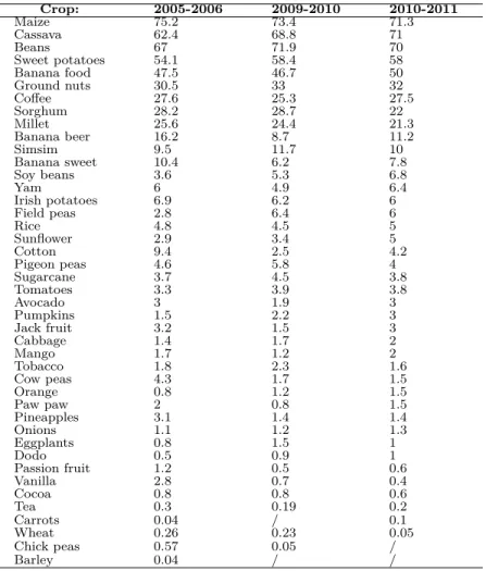
In order to better understand the crop choice patterns of Ugandan farmers, Table A.1 shows the share of households cultivating a given crop and Table A.2 shows the average contribution of each crop to the total value of each household’s production on the raw data (in Appendix). According to Table A.1, the major cereal crops are maize, cassava, millet and sorghum; important vegetables and fruits are beans, groundnuts, sweet potatoes and food banana; the traditional cash crops are coffee and to some extent cotton and sugarcane. What we observe is that, on average, other crops than cash crops are mostly included in the households’ portfolio even if their contribution to the average production value is lower than that of cash crops.

Given these descriptive statistics on the crop choices in the sample, I proceed with con-struction of the different types of dependent variables based on what households cultivate and how they allocate their land. Two different sets of dependent variables will be used in the analysis. The first set includes different diversification indices. The second dependent variable is the weighted portfolio beta which is an average of each beta from a Single Index

(42)

Model estimation for the crops cultivated by a given household. The construction of this variable is explained in detail in Section 1.2.2 and Appendix A.1.

2.2.1 Definition and descriptive statistics on the diversity indices

The first set of dependent variables is constituted of different diversity indices that are adapted from the ecological literature [Baumgärtner, 2006, Smale et al., 2003]. I limit the analysis to the inter-specific aspect of diversity, including the diversity measures of the different crops, but not the different varieties/seeds of a given crop. The diversity indices can be classified into three categories. The first category refers to the simplest measure of diversity, i.e., a richness/count index, and it represents the total number of crops cultivated by a household. The richness index assumes an equal contribution of each crop to the household’s crop diversity. One might argue that different crops should count differently for the degree of diversity. The second category of diversity index, the Berger-Parker index, takes into account the dominance of certain crops over other. According to the definition given in Table 2.1, the lower the share of the land dedicated to the most abundant crop, the higher the value of the Berger-Parker index. The third category of diversity indices, the Simpson index and the Shannon index, include in their definition the richness and the evenness of crops. The evenness refers to the level of equality of the abundance of different crops. A higher value of these indices is due to a higher number of crops but also to a higher equality of the abundance of the different crops. In the present analysis, the latter can be interpreted as equal land shares among different crops. A summary of the definitions is given in Table 2.1.

(43)

T able 2.1 – Definition of the div ersit y indices Index Mathematical calculation Explanation In this c hapter Coun t D = S S -the n um b er of sp ecies in the ec o system S-n um b er of crops c ultiv ated b y the farmer D ≥ 1 Berger-P ark er D = 1 /p max pmax -the most a bundan t sp ecies pmax -the highest land sha re dedicated to a crop D ≥ 1 The higher the abunda nce of the most abundan t sp ecies, the lo w er the index v alue. Shannon D = − P pi lnp i pi -prop ortion or relativ e abunda nce pi -the land share o ccupied b y crop i D ≥ 0 of sp ecies (in v erse) Simpson D = 1 / P p 2 i pi -prop ortion or relativ e abunda nce pi -the land share o ccupied b y crop i D ≥ 1 of sp ecies Sour ce: T able and calculations adapted from Smale e t al. [ 2003 ] and Baumgärtner [ 2006 ]

(44)

In order to construct the different dependent variables, it is necessary to have detailed information on the share of land that farmers dedicate to different crops. The LSMS-ISA data contain this information, but for some households the shares do not sum up to 100 percent.1 _{Thus I restrict the sample to households for which the crop shares, net of fallow}

land, sum up correctly. This implies that we might not have the information for both seasons for all households. I control for this issue by introducing a dummy for whether the agricultural data used are from both seasons, from the first season or from the second season. The attrition rate among the agricultural households between the first (2005/2006) and the second wave (2009/2010) is 11 percent, and between the second (2009/2010) and the third wave (2010/2011) is 9 percent. The number of households that are present in the three waves is 1742. I restrict the sample to those households for which land shares sum to 100 percent, and the final sample comprises 1538 households.

Table 2.2 describes the summary statistics of the dependent variables. The statistics on

the count index show that on average, households planted 5 crops in the period from 2009 to 2011. The average number of cultivated crops increased between the two periods from 4.98 to 5.17. 80 percent of the households cultivated two to six crops and only three percent of the households cultivated only one crop with the median being five crops during the whole period. The other diversity variables are lower than the count index which indicates that land is not equally distributed to different crops. All the three diversity indices are left-censored to zero or one for households that cultivate one crop and their mean value increases from one year to the other. This increase can be due to an increase in the number of cultivated

1_{This is most likely due to interviewer mistakes and therefore I can infer that the error is not correlated}

(45)

crops, but also from a more equal allocation among different crops.

2.2.2 Construction of the measure of riskiness

One of the purposes of the chapter is to construct a riskiness measure of each crop cultivated by a farmer and to compute the overall riskiness of the farmer’s crop production. To do so, I will use the Single Index Model (SIM) used, among others, byTurvey[1991] and by Bezabih and Di Falco [2012]. Unlike the Capital Asset Pricing Model (CAPM), SIM is

not an equilibrium model and can be applied to any portfolio. This is an argument for the application of the SIM on African agriculture where markets are incomplete.

The Single Index Model assumes that the revenues associated with various farm enter-prises are related through their covariance with some basic underlying factor or index. The risk correlated with this index is called non-diversifiable or systematic risk and the second risk component is the part of farm returns that is not correlated with the index, called spe-cific risk that can be completely diversified. The systematic risk can be determined by a reference portfolio defined as:

Ipht = n

X

i=1

wihtIiht (2.1)

where wiht refers to the land weights of crop i for household h in the time t and Iiht are the

stochastic crop revenues. A parameter that measures the anticipated response of a particular crop to the changes in portfolio returns needs to be estimated. This coefficient, βi, is given

by a panel regression of Iiht on the reference portfolio Ipht:

(46)

T able 2.2 – Summary statistics of the dep enden t v ariable s T otal 2009/2010 2010/2011 V ariable M ean SD Min Max Mean SD Min Max Mean SD Mi n Ma x R isk variable w eigh ted p ortfolio b eta 0.28 0.50 0 7.60 0.29 0.55 0 7.60 0.28 0.4 5 0 6 .0 8 Inter-sp ec ific diversity variables coun t index n 5.07 2.05 1 16 4.98 2.06 1 13 5.17 2 .0 4 1 16 in v erse Simpson 3.36 1.35 1 9.40 3.27 1.31 1 8.08 3.48 1.39 1 9.40 Shannon 1.28 0 .4 2 0 2 .3 0 1.25 0.43 0 2.27 1.32 0.42 0 2.30 Berger-P ark er 2.40 0.87 1 6.79 2.34 0.83 1 5.69 2.46 0.90 1 6.92

(47)

By definition βi = σipht

σ2

pht

which means that βi is a sufficient measure of marginal risk. Beta

coefficients are estimated with the Equation (2.2) by using a panel fixed effects model in order to account for the unobserved household characteristics. The portfolio beta coefficient is calculated as a weighted average of the beta coefficients estimated for each crop that the household cultivates. A more detailed explanation of the SIM is given in Appendix A.1.

Table 2.3 gives the estimates of different crop beta coefficients. We can interpret these coefficients in the following way: if we consider, for example, cotton and maize, we observe that an increase in the reference portfolio of 1 Ugandan Shilling (UGX) will induce a more than proportional increase of the cotton revenue of 1.22 UGX and no increase in the maize revenue. These estimates indicate that cotton is riskier than the average crop portfolio, whereas maize has a more stabilizing effect. The estimates of the beta coefficients are consistent with the agricultural and economic literature on riskiness of crops.

Table 2.3 – Estimation results: Beta Coefficients

Crop Coefficient Crop Coefficient

sweet potatoes 0 sorghum 0.22

cassava 0 beans 0.25 maize 0 avocado 0.36 millet 0 mango 0.43 pumpkins 0 simsim 0.50 dodo 0 tomatoes 0.50 vanilla 0 pineapples 0.52

paw paw 0.02 oranges 0.63

rice 0.03 banana 0.70

eggplants 0.04 tea 0.78

pigeon peas 0.08 irish potatoes 1.05

banana beer 0.10 cotton 1.22

soy beans 0.11 field peas 2.00

ground nuts 0.12 sunflower 2.00

yam 0.13 cabbage 2.31

onions -0.13 cocoa 3.23

banana sweet 0.14 passion fruit 3.69

coffee 0.15 tobacco 5.25

Jack fruit 0.20 sugarcane 7.96

According to Table 2.2 the mean portfolio beta is relatively low (0.28). The minimum

is 0, which means that the crop portfolio does not react to the variation of the reference portfolio. The maximum is 7.60 which means that an increase of 1 UGX in the reference portfolio provokes an increase of 7.60 UGX in the given portfolio.

(48)

2.2.3 Definition and descriptive statistics of the explanatory

vari-ables

Table 2.4 presents definitions and the summary statistics of the explanatory variables that are used in the estimations. Summary statistics are given for the whole sample, column (All HHs), for the share of households that do not receive remittances, column (Non-Rem HHs) and for the share of households that receive remittances, column (Rem HHs). A difference in means between these two groups is reported, to test for any differences of the characteristics between the two groups of households. The main variable of interest is the lagged level of remittances that a household receives from its migrants. About 35 percent of the households in the data-set reported that they received remittances locally or from abroad. The mean value of remittances is 101 000 UGX per household. Among the households receiving remittances, the average is 315 000 UGX. Intuitively, the district average of remittances is lower for households that do not receive remittances compared to those that receive remittances.

Based on the descriptive statistics of the whole sample, household heads have on average 48 years, are mostly male (about 70 percent) and have on average attended only primary school. The average number of male and female adult members of the households is around 3 and the average dependency ratio is 1.70, which indicates that for every adult worker there is 1.70 household members of non-working age. The average assets are around 5 780 000 UGX and the average non-agricultural income is higher than the average level of remittances which may question the strength of the role of remittances as insurance . About half of the households are credit-constrained. This variable takes value 1 if a household was refused to

(49)

T able 2.4 – Definition and descriptiv e statistics of the explanatory v ariables on the whole sample and b y group of HHs V ariable Definition All HHs Non-Rem HHs Rem HHs Dif in Means R emittanc es remittances receiv ed b y the hh from migran ts 101 0 315 -315*** lo cally or abroad in t-1 (UGX) ditlev elremit mean district lev e l of remittances t-1 (UGX) 101 94 126 -32*** Household char acte risti c s sex the gende r of the hh head 0.71 0.79 0.52 0.273*** equals 1 if the hh head is male age the age of the hh head 47.8 45.6 52 .4 -6.86*** education the highest sc ho o l lev el ac hiev ed b y the hh head 1.01 1.03 0.97 0.06 0-no education, 1-primary , 2-secondary edumax the n um b er of y ears of sc ho oling of the most e ducated 8.5 8.4 8.7 -0.3** hh mem b er in t − 1 a v erageduc a v erage n um b er of y ears of sc ho oling of all 4.75 4.67 4.89 -0.22*** hh mem b ers in t − 1 madults male hh mem b ers b et w een 16 and 65 y ears 2.89 3.02 2.61 0 .4 2*** fadults female hh mem b ers b et w een 16 and 65 y ears 3.04 3.13 2.85 0.28*** dep. ratio the dep endency ratio of the hh 1.70 1.60 1.76 -0.16 W ealth char acteristics non-agricultural income income fr om non agricultural activities (UGX) 588 678 397 281*** assets total assets in monetary v alue (UGX) 5 780 4 050 9 430 -5 380*** credit constrain t credit constrain t dumm y 0.50 0.50 0.50 0 equals 1 if the household is constrained, 0 otherwise L and char acte ris tic s land land o wnings in acres 3.21 3.41 2.80 0.61 qualit y index w eigh ted index of soil qualit y 1.43 1.43 1.44 -0.01 with: lev el 1 b eing go o d qualit y and lev el 3 b eing p o or qualit y W eather char acteristics rain rain deviation in t − 1 in district d from the long run mean 0.28 0.29 0.27 0.02** divided b y the long run stan dard deviation in absolute terms temp eratur e temp erature deviation in t − 1 in district d from the long run mean 2.39 2.36 2 .44 -0.08*** divided b y the long run stan dard deviation in absolute terms Observ ations 3 076 2 087 989 Note: All categories of rev en ues are in thousands of Ugandan Shillings (UGX). F or example the a v erage lev el of remittances for all ho use ho ld s are 101 000 UGX. The exc hang e rates of Ugandan Shillings p er US dollar for Jan uary 2009, 2010 and 2011 are resp ectiv ely 1 976, 1 936 and 2 332. The a v erage land o wnings corresp ond to 1.3, 1.4 and 1.13 hect a res.