HAL Id: dumas-01095979
https://dumas.ccsd.cnrs.fr/dumas-01095979
Submitted on 16 Dec 2014
HAL is a multi-disciplinary open access
archive for the deposit and dissemination of
sci-entific research documents, whether they are
pub-lished or not. The documents may come from
teaching and research institutions in France or
abroad, or from public or private research centers.
L’archive ouverte pluridisciplinaire HAL, est
destinée au dépôt et à la diffusion de documents
scientifiques de niveau recherche, publiés ou non,
émanant des établissements d’enseignement et de
recherche français ou étrangers, des laboratoires
publics ou privés.
Polarization: The Role of Productivity and Taxation
Sébastien Bock
To cite this version:
Sébastien Bock. Structural Transformation and Labor Market Polarization: The Role of Productivity
and Taxation. Economics and Finance. 2014. �dumas-01095979�
UFR 02 - Sciences Economiques
Master 2 Recherche Economie Théorique
et Empirique
Structural Transformation and Labor Market Polarization:
The Role of Productivity and Taxation
Directeur de soutenance : Monsieur François Langot Présenté et soutenu par : Sébastien Bock
Are productivity growth and taxation accountable for the
evolution of low skilled service hours worked in Europe and the
United States?
Sébastien Bock
Abstract
This article aims at deepening our understanding on three main facts in labor economics: the process of structural transformation, the labor market polarization and the deterioration of European labor market out-comes. The literature has focused on two main sources that explain these phenomena i.e. productivity growth and taxation. In order to under-stand the allocation and the evolution of hours worked, the literature has also insisted on the importance of studying more disaggregated features. The originality of our approach is to extend the literature by focusing on the role played by productivity growth and taxation in low skilled service hours of work. Indeed, this sector produces services that can be highly substitutable with home produced goods. One might expect that taxa-tion has a significant impact on hours worked in this sector. In order to study those relations, we built a general equilibrium task model with a good and a service sector. We allowed for Information and Commu-nication Technology (ICT) diffusion which is equivalent to productivity growth. We also introduced distortionary taxation on labor income and a home production sector which is not subject to taxation. Our model suc-ceeded at replicating some qualitative facts on variables as hours worked, relative prices and wage polarization. We also aimed at replicating the shares of hours worked in the good and the service sectors in the case of Europe suggesting that productivity growth and taxation are indeed key variables.
Contents
1 Introduction 4
2 Stylized Facts 6
2.1 Aggregate Hours of Work and Taxation . . . 6
2.2 Sectoral Hours of Work . . . 9
3 A General Equilibrium Task Model 16 3.1 The Supply Side . . . 16
3.1.1 The Good Supply Sector . . . 17
3.1.2 The Service Supply Sector . . . 19
3.1.3 The Equilibrium . . . 20
3.2 The Demand Side . . . 21
3.3 Market Clearing Conditions and the Government Constraint . . . 22
3.4 The General Equilibrium . . . 23
3.5 Asymptotic Allocation of Hours Worked . . . 24
3.5.1 Preliminary Computations . . . 24
3.5.2 Asymptotic Wages . . . 25
3.5.3 Asymptotic Allocation of Hours Worked . . . 25
3.5.4 Asymptotic Wage Ratios . . . 26
3.6 Intuitions . . . 28
4 Calibration 28 5 Results 29 5.1 Hours of Work and Taxation . . . 29
5.2 Wages, Prices and Consumption . . . 30
5.3 Wage Polarization . . . 30
5.4 Share of Hours Worked . . . 30
List of Figures
1 Hours Worked in Europe and the U.S. - Total . . . 7
2 Hours Worked by Country - Total . . . 8
3 Hours Worked compared to the U.S. . . 8
4 Labor Income Tax Rates . . . 9
5 Hours Worked - Good and Service Sectors . . . 12
6 Hours Worked by Country - Good and Service Sectors . . . 12
7 Shares of Hours Worked - Good and Service Sectors . . . 14
8 Shares of Hours Worked - All Sectors . . . 14
9 Shares of Hours Worked - Service Sector . . . 15
11 Model - Wage Polarization . . . 32
12 Theoretical Shares in Hours of Work . . . 32
10 Model - Rise in Productivity of Capital . . . 33
List of Tables
2 Sectoral Decompositions . . . 131
Introduction
During the second half of the 20th century, the European and the US labor markets have known significant changes. This paper aims at deepening our un-derstanding on three of them by looking at disaggregated features.
Firstly, there has been a process of structural transformation. Indeed, both Europe and the United States have seen their labor force reallocated from the manufacturing good sector to the service sector. This was mainly due to the evolution of productivity in each sector. As Kuznet (1966) has discovered, as a country becomes more and more productive, labor is reallocated from the man-ufacturing good sector to the service sector.
Secondly, those two entities (Europe and the U.S.) have also experienced job and wage polarization since the 80s. Hours worked and employment have in-crease both at the bottom and at the top of the skill and wage distributions. Wages have followed the same pattern even if European and U.S. institutions are different.
Thirdly, hours worked have decreased in Europe compared to the US. There has been a deterioration of European labor market outcomes. Given the Kuznet stylized facts, this last observation should be at odds with one’s expectations. Indeed, one might expect that the European and the U.S. labor markets should have converged in terms of hours of work and structure. In fact, other variables and mechanisms have to be taken into account such as the role of taxation and public spendings in order to deepen our understanding of the evolution of hours worked.
The literature has already been widely developed. In fact, we are at the intersection of two main frameworks: structural transformation and labor mar-ket polarization. On the one hand, the literature on structural transformation has focused mainly on the extension of the standard growth model in order to explain the allocation of labor from the agricultural sector to the manufacturing good sector and then from this last sector to the service sector. Indeed, those papers usually aim at reproducing the process of labor reallocation across sectors by either using the demand- or supply-side mechanisms with a growth device. Kongsamut, Rebelo and Xie (1998) have developed a multisector neoclassical growth model that preserves the balanced growth properties but also succeeds at replicating the unbalanced properties of growth, i.e. the reallocation of resources across sectors. Acemoglu and Guerrieri (2006) have focused on a supply-side mechanism in order to study the structural transformation. They developed a multisector growth model. Each sector uses relatively more or less capital in its production. The growth device of this model is capital deepening. There-fore, as capital accumulates, the relative output of the capital intensive sector increases but it also generates a reallocation of capital and labor away from this sector inducing a reallocation of resources towards more labor-intensive sectors. In constrast with the previous paper, Ngai and Pissarides (2008) focused on a demand-side mechanism. They developed a multisector growth model with a home production sector and total factor productivity growth in order to repli-cate both aggregate and sectoral evolutions of hours worked in the U.S.. Total factor productivity changes imply a rise of the relative price of services lead-ing to structural transformation whenever the elasticity of substitution between goods is different from one. Boppart (2011) also focused on a demand-side mechanism. He built a sectoral growth model with non-homothetic preferences
in contrast with the previous paper. By using non Gorman preferences, he could focus on the interaction between growth and preference specification. The main idea is that as households become richer with total factor productivity growth and relative prices changes, their consumption structure changes over time due to the interaction between income and substitution effects. Rogerson (2007) designed a model to provide the literature with a comparative analysis between Europe and the U.S.. He focused on the role played by productivity growth and taxation in order to explain both the structural transformation and the relative deterioration of the European labor market outcomes. He found that while the two entities have experienced structural transformation, Europe didn’t see its hours worked reallocated to the service sector to the same extent as the U.S.. According to him, this is due to the disincentive to work generated by the high tax rates on labor income implemented in Europe.
On the other hand, the literature on labor market polarization has focused on explaining more disaggregated features. It has focused on hours worked by sec-tors, skill levels and the evolution of wages. Autor, Katz and Kearney (2006) studied labor market polarization in the U.S.. They found that between the late 1980s and the 2000s employment shares increased both at the bottom and the top of the skill distribution. Furthermore, wage inequality at the top of the income distribution increased for more than twenty five years. However, it stopped for the bottom of the wage distribution since the late 1980s. One key explanation lays in demand shifts but also the diffusion of computarization technologies. Goos, Manning and Salomons (2009) investigated the same phe-nomenon but in European countries. They also found that as in the U.S. there has been both job and wage polarizations despite differences in institutions. Indeed, their results show that employment shares in Europe increased for the highest and the lowest pay distributions while decreasing for the middling pay distribution. Those findings were quite robust when they looked at each country separately. One main explanation is that technological progress led to the real-location of labor towards occupations at the bottom and the top of the income distribution. This is due to the computarization of middling occupations of the income distribution. Galbis and Sopraseuth (2011) confirmed those findings in the case of France and also added aging as an important factor to job polariza-tion. Autor and Dorn (2013) have also studied labor market polarizapolariza-tion. They have focused on the evolution of low skilled service jobs. They found that the diffusion of information and communication technologies (ICT) has led to the reallocation of the labor force from the good sector intensive in routine tasks to the personal service occupations which are intensive in manual tasks.
In this paper, we deepen the comparison made by Rogerson (2007) between Europe and the United States by investigating the role played by productivity growth and taxation in the reallocation of hours worked across specific sectors. Indeed, as suggested by the literature, we study more disaggregated features. More precisely, we focus on the influence of productivity growth and taxation on the evolution of hours worked in the personal service sector. In other words, are productivity growth and taxation accountable for the evolution of low skilled service hours worked in Europe compared to the United States?
In section 2, we document the reader with stylized facts and observations taken mostly from the EU KLEMS database used also by Rogerson in order to have comparable results with this study. In section 3, we build a general equilibrium task model that aims at replicating three main facts described in
labor economics and found in our dataset: structural transformation, labor market polarization and the relative deterioration of European labor market outcomes. In order to do so, we based our model on the work of Rogerson (2007) and Autor and Dorn (2013). In section 4 and 5, we expose respectively the calibration used and our results. Finally, in section 6, we conclude our study and explain some major questions that remain open in order to understand the reallocation of hours of work.
2
Stylized Facts
In this second section, we present some important stylized facts that we aim at replicating. In order to do so, we use sectoral data taken from the EU KLEMS database, population data from the OECD database and labor income tax time series from the work of McDaniel (2007). We also take some aggregated data from the Penn World Table database of the Groningen Growth and Development Centre. Furthermore, since we study the long run allocation of hours worked, we filter our data with the Hodrick and Prescott time series filter with a smoothing parameter of λ = 100 as recommended by the literature when we use annual time series. Firstly, we will focus on aggregate stylized facts and then we will look at more disaggregated features by looking at different sub-sectoral levels. We will mainly study two entities which are the United States and Europe in which we include Belgium, France, Germany, the Netherlands, Italy and the United Kingdom.
2.1
Aggregate Hours of Work and Taxation
In order to be able to compare hours worked between countries and entities, we have to study hours worked relative to the working age population:
h15−64 = Total Hours Worked by employees
Working age Population 15-64
In Figure 1, we report the evolution of total hours worked by the working age population. It is clear that from 1970 to 2007, there has been a decrease in hours worked in Europe while there has been an increase in hours of work in the United States. This evolution is not due to only one or few European countries. It is a global phenomenon that seems to be shared by most of the European countries that we are considering. Indeed, when we look at Figure 2, most countries have seen their hours of work relative to their working age population decrease over time. At least, the level of this ratio in 1970 is higher than in 2007 except for Italy. Furthermore, by observing Figure 3, we can see that relative hours worked in European countries taken individually decrease with respect to hours worked in the United States. For example, in the case of Belgium, France, Germany and the Netherlands, one can notice that in 1970, those countries had higher absolute hours worked with respect to those of the U.S.. They were approximately 1.02 to 1.1 times higher in Europe than in the United States. In 2007, hours worked in those countries were between 0.8 and 0.95 times those of the United States. Clearly, there has been a deterioration of labor market outcomes at least with respect to the United States as Rogerson (2008) reported. One plausible explanation among others is the rise in taxation
in France compared to the U.S.. In fact, according to Figure 4, one can observe that labor income tax rates are significantly higher in all the European countries than in the United States. Furthermore, almost all European countries have seen their labor income tax rate rise at a higher speed than the United States except for the Netherlands which still have a higher labor income tax rate. Since we want to study a European entity, we build a population-based labor income tax rate index the same way Rogerson (2008) did:
τEU = P i∈I P opiτi P i∈I P opi
with I = {Bel, F r, Ger, Nld, It, UK}. It is clear that Europe as we designed it, has a higher tax rate relatively to the U.S.. It starts from a value of 25% in 1970 to reach 35% in 2007 while for the U.S. those values are respectively 17% and 20%. Those differences in tax rates are clearly linked to the evolution of hours worked in Europe and the United States. Many papers have tried to identify those links as for example Rogerson (2006), Rogerson (2008), Prescott (2004).
1970 1975 1980 1985 1990 1995 2000 2005 900 950 1000 1050 1100 1150 1200 1250 1300
Hou r s Wor k e d by 15-64: Tot al
Ye ar Hou rs W o r k e d / P op 15-64 E u r op e US
Source: EU KLEMS Database
Source: EU KLEMS Database
Figure 2: Hours Worked by Country - Total
1970 1975 1980 1985 1990 1995 2000 2005 0.85 0.9 0.95 1 1.05 1.1
Av e r age Hou r s Wor k e d Re l at i v e To T h e US
Ye ar Re la t iv e A v e r a g e H o u r s W o r k e d B e l Fr G e r I t Nl d UK
Source: Penn World Table Database
Source: McDaniel (2007) Database
Figure 4: Labor Income Tax Rates
2.2
Sectoral Hours of Work
In this paper, we have choosen to focus on sectoral features in order to under-stand the evolution of hours worked. More precisely, we have decided to focus on the impact of productivity growth and taxation on the personal service sector which is a low-skilled service sector. In this sense, we deepen previous studies made on the polarization of the European and the U.S. labor markets and also on Structural Transformation. Indeed, we focus mainly on two of them: Roger-son (2008) and Autor and Dorn (2013). RogerRoger-son (2008) investigated the role of productivity growth and taxation in the process of structural transformation. However, when he built his service sectors, he used a very heterogeneous set of sub-sectors. Indeed, his service sector includes for example the financial sector, the personal service sector, the distribution and trade sectors. All those sectors do not produce close substitutes to home produced goods. Therefore, it is im-portant to build a relevant service sector. We have decided as Autor and Dorn (2013) did to focus on the low-skilled service sector and more precisely on the personal service sector which is probably the sector that produces the closest substitutes to home produced goods. In this sector, one can find restaurants, hotels, other community and personal services but also private households with employed personal. Figure 5 clearly shows that hours worked in the good and service sectors, as defined in Table 2, have decreased over time in Europe while they have increased in the United States. Thus, the deterioration of European labor market outcomes compared to the United States comes surely to some extent from the evolution of hours worked in the good sector. However, in the service sector as we define it, we can see that hours worked are increasing both in the United States and in Europe. We observe the process of structural
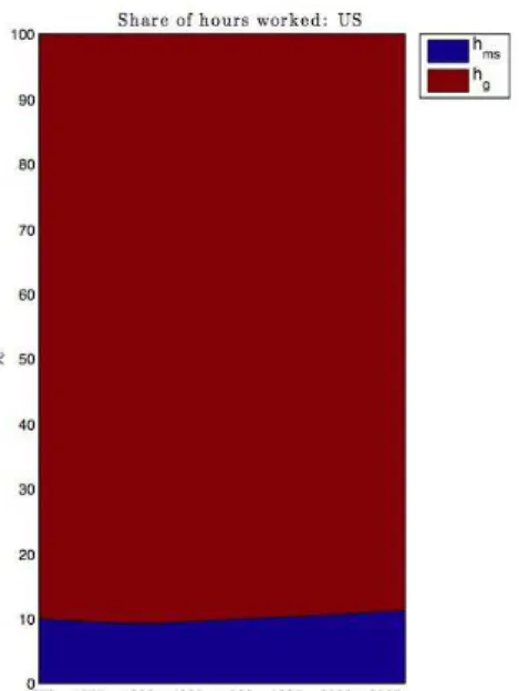
transfor-mation described by Rogerson. Indeed, there seems to be a reallocation of hours worked from the good sector to the service sector. However, we can also see that those hours worked are lower in Europe than in the United States showing again that labor market performance is higher in terms of hours worked in the United States than in Europe. As one can notice in Figure 6, this phenomenon is not country specific. Indeed, this reallocation process from the good sector to the service sector is shared by almost all of the sub-countries used to build our European entity. Nevertheless, even if we focus on common facts that seem to link those countries, there are still country-specific features which need to be studied in future research. For example, one can see that hours worked in the good sector in Italy are very low and even increase in 2007 compared to 1970 in contrast to other countries. One can also notice that Italy has seen its hours worked in the service sector increase much more than in any other country. Therefore, we decided to ignore those country-specific features in order to focus on more common trends. Figure 7 shows the evoluation of shares of hours of work in the good and the service sectors in both the U.S. and Europe. One can remark that in Europe, the share of hours of work in the service sector has risen from 5% in 1970 to 10.9% in 2007. In the United States, it is less visible but the service sector share has grown from 9.9% to 11.2%. Therefore, the share of hours worked in the service sector is higher in the United States than in Europe reflecting again the deterioration of European labor market outcomes but it still seems that there is some process of structural convergence in sectoral shares be-tween those two entities. In the next section, we build a model that aims at replicating both the relative deterioration of European labor market outcomes and the evolution of sectoral shares which describes more accurately the process of structural transformation.
Finally, we expose more disaggregated sector shares in order to see which of those subsectors drive those stylized facts. In Figure 8, we decompose hours worked in seven sectors as described in Table 2. It shows that in Europe most of the reduction in hours worked in the good sector as we define it comes from the manufacturing good sector and the other good production sectors which include for example the agricultural sector, the construction sector and the electrical machinery, post and communication services sector. Indeed, the share of those sectors falls from 55% to approximatively 30% of total hours worked. However, some subsectors in the good sector see their share of hours worked increase, such as the finance and business sectors or the non market sector which includes for
example education, the public administration1. Those sectors are usually taken
into account in the service sector but since we focus on the personal service sector which corresponds to our service sector, we include those sectors in our good sector. Finally, the share of hours worked in the personal service sector increases over time. One can observe a similar evolution of shares in the United States. Indeed, the share of the manufacturing good sector and the other good production sectors decreases from approximatively 48% to around 25% while the share of the service sector rises as previously shown. Finally, by disaggre-gating to an even lower level (20 sectors), we can see which are the sectors that drive the rise in the service sector share in total hours of work. In Europe, hours worked as a share of total services in hotels and restaurants (N) remained
sta-1
This last subsector includes the defense sector which we would have liked to suppress if more disaggregated data were available.
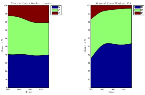
ble at approximatively 40% from 1970 to 2007. Meanwhile, the share of other community and personal services (O) has decreased from around 47% to 40% of total hours worked in the service sector. In contrast, the share of hours of work in the private households with employed persons has increased substan-tially from approximatively 12% in1970 to 20% in 2007. In the United States, service sectoral shares differ with respect to European shares. Indeed, hours worked as a share of total hours of work in the service sector rise in hotels and restaurants (N) from around 35% in 1970 to more than 50% in 2007 while the share for the private households with employed persons (P) falls from around 16% in 1970 to less that 5% in 2007. Again, one should not forget that the European entity might hide country specific entities even if less disaggregated features are generally shared by these countries.
1970 1975 1980 1985 1990 1995 2000 2005 800 850 900 950 1000 1050 1100 1150 Hou r s Wor k e d by 15-64: G o o d s Ye ar Ho u rs W o rk e d / P o p 1 5 -6 4 E u r op e US 1970 1975 1980 1985 1990 1995 2000 2005 60 70 80 90 100 110 120 130 140 Hou r s Wor k e d by 15-64: S e r v i c e s Ye ar Ho u rs W o rk e d / P o p 1 5 -6 4 E u r op e US
Source: EU KLEMS Database
Figure 5: Hours Worked - Good and Service Sectors
1970 1980 1990 2000 600 700 800 900 1000 1100 1200 1300 Hou r s Wor k e d by 15-64: G o o d s Ye ar Hou rs W or k e d /P op 15-64 B e l Fr G e r I t Nl d UK 1970 1980 1990 2000 40 50 60 70 80 90 100 110 120 130 140 Hou r s Wor k e d by 15-64: S e r v i c e s Ye ar Hou rs W or k e d /P op 15-64 B e l Fr G e r I t Nl d UK
Source: EU KLEMS Database
L IZE D F A CTS 13
2 Sectors 7 Sectors 20 Sectors
Goods
Electrical Machinery and ELECOM Electrical and Optical Equipment A Post and Communication Services Post and Telecommunications B Consumer Manufacturing C Total Manufacturing MexElec Intermediate Manufacturing D (excl. Electrical) Investment Goods, excluding Hightech E Other Production OtherG
Mining and Quarrying F Electricity, Gas and Water Supply G
Construction H
Agriculture, Hunting, Forestry and Fishing I Distribution DISTR Transport and StorageTrade KJ Finance and Business
FINBU
Financial Intermediation L Renting of m&eq and
M (excl. Real Estate) other business activities
Non Market Services NONMAR
Public Admin and Defense;
Q Compulsory Social Security
Education R
Health and Social Work S Real Estate activities T Services Personal Services PERS
Hotels and Restaurants N Other Community, Social and
O Sersonal Services
Private households with employed persons P Table 2: Sectoral Decompositions
Source: EU KLEMS Database
Figure 7: Shares of Hours Worked - Good and Service Sectors
Source: EU KLEMS Database
1970 1980 1990 2000 0 10 20 30 40 50 60 70 80 90 100 S h ar e of Hou r s Wor k e d : E u r op e T i me Sha r e in % N O P 1970 1980 1990 2000 0 10 20 30 40 50 60 70 80 90 100 S h ar e of Hou r s Wor k e d : U. S . T i me Sha r e in % N O P
Source: EU KLEMS Database
3
A General Equilibrium Task Model
In this section, we build a general equilibrium task model that aims to deepen our understanding of three main facts described in labor economics by looking at disaggregated features. The first one is structural transformation. Thus, our model must have a sectoral dimension in order to replicate the evolution of the share in hours worked in the good and service sectors. The second fact is job and wage polarizations. Indeed, usually structural transformation and job polarization have been treated separately in the literature. However, we believe that they are very closely related. Furthermore, in many papers, au-thors don’t study the relation between the reallocation of labor across sectors and the evolution of wages. Since the literature and the data have shown clear evidence on the heterogeneity of the evolution of wages, we believe that our model must take into account a certain measure of inequality in income and skills in order to replicate wage polarization. The third and last fact is the European deterioration of labor market outcomes compared with the US. With similar institutions and environment, the European labor market should have converged towards the U.S. in terms of sectoral hours worked according to the evolution of productivity. The reduction in hours worked in the good sector should have been compensated by an important increase in hours worked in the service sector. This has not happened with the same intensity as in the US labor market. The literature has underlined the potential important role of taxation and thus of fiscal policy. This leads us to the following question: are productivity growth and taxation accountable for the evolution of low skilled service hours worked in Europe compared to the United States? Therefore, in order to answer this question, we believe that our model should introduce some kind of distortionary taxation with a domestic production sector that absorbs hours of work. In order to do so, we based our model on the works of Rogerson (2007) and Autor and Dorn (2013). The former studies structural transforma-tion and in particular the impact of productivity and taxatransforma-tion while the latter focus on job and wage polarizations through the diffusion of Information and Communication Technologies (ICT).
3.1
The Supply Side
We consider three main sectors which are perfectly competitive: a good sector, a service sector and a home production sector. The service sector represents per-sonal services and uses intensively manual tasks. The good sector is composed of all other sectors. Therefore, there will be for example the manufacturing good sector and the finance and business sector. This decomposition allows us to focus on low skill service hours of work. We also consider three inputs: high skilled labor, low skilled labor and capital. Each worker is characterized by a set of skills {a, r, m} for respectively abstract, routine and manual tasks. High skilled labor is only used to do abstract tasks and consequently is characterized
by the set of skill levels {1, 0, 0}2. Low skilled labor is used to accomplish two
types of tasks which are routine and manual tasks. Low skilled workers have the same ability to accomplish manual tasks. However, they are heterogenous
2
We could have assume instead that high skilled workers have a set of skills {1, 1, 1} with wa> wr, wm. Thus, high skilled workers would always choose to produce abstract tasks.
according to their skill level in efficiency units η ∈ [0; +∞] for producing
rou-tine tasks. η is characterized by its density function f(η) = e−η as in Autor
and Dorn (2013). Consequently, each low skilled worker is characterized by a skill level {0, η, 1}. Capital substitutes for low skilled labor only in order to accomplish routine tasks.
3.1.1 The Good Supply Sector
The Production of Goods
Firms in the good sector maximize their profit subject to their production function. Their technology is characterized by the fact that they use abstract tasks, routine tasks and capital as inputs. Therefore, the good supply represen-tative firm program is:
Πg = max Yg− pkK− wrhr− waha
s.t. Yg≤ h1−βa [(Arhr)µ+ (AkK)µ]
β µ
with hr, ha hours worked in routine and abstract tasks, K and pk capital
and its price, and µ, β ∈ [0; 1]. We implicitly assume that the price of the good is normalized to one. The intuition is that in order to produce a good, the producer has to combine abstract labor with an intermediary good X = [(Arhr)µ+ (AkK)µ]
1
µ which is produced with routine labor and capital. The
elasticity of substitution between abstract tasks and total routine tasks both accomplished by low skilled workers and capital is equal to 1 while the elasticity of substitution between routine tasks accomplished by low skilled workers and
those produced by capital is σr = 1−µ1 . We will assume that low skill labor
routine tasks are close substitutes of capital which means that σr>1 or µ > 0.
This means that if the price of capital falls, then firms in the good sector will tend to substitute capital for labor routine tasks. Thus, there is a mechanism of reallocation of low skilled labor linked to the diffusion of capital. We will see that when this happens, the low skilled labor is reallocated from the good sector to the service sector. In other words, some of the low skilled workers will no more produce routine tasks but they will instead accomplish manual tasks. The first order conditions for routine and abstract tasks are respectively:
wa = (1 − β) h−βa [(Arhr)µ+ (AkK)µ] β µ wr = βAµrhµ−1r ha1−β[(Arhr)µ+ (AkK)µ] β µ−1
Thoses equations describe the wage rate for workers that accomplish respectively abstract tasks and routine tasks. The first order condition for capital is:
pk = βAµkKµ−1h1−βa [(Arhr)µ+ (AkK)µ]
β µ−1
Finally, since low skilled workers can choose to work either in the good or the service sectors and thus accomplish either routine or manual tasks, we need a condition in order to determine their labor supply for each of the two types of tasks. A low skilled worker will decide to accomplish routine tasks and thus work in the good sector if:
ηwr ≥ wm
Thus, we assume that there is a threshold level η such that when a low skilled worker has a skill level η > η, he will choose to accomplish routine tasks. When a low skilled worker is characterized by η < η, he will accomplish manual tasks. We can find the labor supply for the good sector as a function of η:
hr = ˆ +∞ η ηdF(η) = ˆ +∞ η ηf(η) dη = ˆ +∞ η ηe−ηdη = (1 + η) e−η
The threshold level η will be solved within the general equilibrium framework in interaction with the demand side of the economy. It is determined endo-geneously. Since high skilled workers can only work in the good sector and accomplish abstract tasks, we get that:
ha = 1
In other words, high skilled workers will allocate their entire time endowment to abstract tasks.
Capital
Capital is produced and supplied in a competitive framework exactly as in Autor and Dorn (2013). The production technology of capital is described by:
K = Yk
eδt
θ
with Yk the amount of goods used to produce capital, δ > 0 and θ = eδ an
efficiency term. We assume that capital fully depreciates at each period. In contrast with Rogerson (2007) technological progress comes from the term δ which represents the growth rate of productivity. The price of capital is:
pk =
Yk
K
One can note that at the beginning of time t = 0, the price of capital is equal to one. Then, as time passes, the price of capital decreases until it converges to zero.
3.1.2 The Service Supply Sector
This sector can be decomposed in two sub-sectors. There is a market service sub-sector which is perfectly competitive and a domestic home production good sub-sector which provides no wages but is not taxed since it’s a non market sector. This last information will matter when we will consider the demand side of the economy.
The Market Service Sector
The representative firm in the market service sector maximizes its profit sub-ject to its production function. Its technology is simpler than in the good sector. Indeed, it only uses low skilled labor in order to accomplish manual tasks. Its program is:
Πs = max pYs− wmshms
s.t. Ys≤ Amshms
with p the relative price of services relative to goods ps
pg since we have normalized
the good price to one. The first order condition for manual labor is:
wms = Amsp
This equation describes the wage provided for manual tasks in the market service sector. In order to find labor supply for manual tasks, we need to consider two things. Firstly, low skilled workers can choose to allocate their hours of work either to the service market sector or to the home production sector. Secondly, manual tasks are done by workers characterized by a skill level η < η. Therefore, we have:
hs = hms+ hmh
which states that the total hours allocated to the service sector is equal to the sum of the hours worked in the market and the home service sectors. We therefore have: hs = ˆ η 0 e−ηdη = ˆ η 0 f(η)dη = 1 − e−η
The intuition is that the allocation of hours worked is sequential. First, low skilled workers determine whether they will work in the good or the service
sectors and thus whether they will accomplish routine or manual tasks. Then, they will decide how to allocate their hours of work for services either to the market service sector or to the home production sector.
The Home Production Sector
We assume that household production technology only uses manual tasks. This assumption is quite realistic since this sector produces for example substi-tutes for restaurants or gardening.The home production sector is characterized only by a production function:
Yh = Ahhmh
with hmh hours worked in home production manual tasks. Hours worked in
the home production sector can vary. For example, if we assume that Yh is
constant and that the productivity parameter Amhincreases exogenously, there
must be less hours worked in the home production sector in order to achieve the same level of output. The role of this sector is to produce a close substitute to market service sector production. While the wage obtained by working in the market service sector is subject to taxes, the home production activity doesn’t pay any wage but is entirely protected from taxation. Consequently, we can conjecture that when the tax rate increases then low skilled workers will tend to reallocate some of their worked hours from the market service sector to the home production sector. This mechanism can help us to replicate the relative fall in hours worked in European countries compared with the US.
3.1.3 The Equilibrium
The supply side equilibrium is characterized by eleven equations: wr = βAµrhµ−1r ha1−β[(Arhr)µ+ (AkK)µ] β µ−1 wa = (1 − β) h−βa [(Arhr)µ+ (AKK)µ] β µ pk = βAµkKµ−1h1−βa [(Arhr)µ+ (AkK)µ] β µ−1 wms = Amsp η = ws wr hms+ hmh = 1 − e−η hr = (1 + η) e−η ha = 1 pk = θe−δt Yms = Amshms Yh = Ahhmh
For now, we have eleven equations for eleven unknown variables "wr, wms, wa, pk,
3.2
The Demand Side
On the demand side of the economy, the representative consumer chooses its levels of consumption for services, goods and home produced goods given prices and wages. He also has to choose its labor supply which we partly defined in the previous sub-section. Indeed, we defined the condition under which a low skilled worker will prefer to accomplish routine or manual tasks and thus whether he will work in the good sector or the service sector. We also defined high skilled worker’s labor supply. In this section, we describe another choice that the representative agent has to make. Indeed, he has to choose the amount of time he is willing to dedicate to market work and to home production work. This choice is central in this model due to the presence of taxation. The representative household can either work in the market sector and then receive a net wage diminished by distortionnary taxation or he can dedicate some of his time to home production and receive no wage but the gain obtained from this sector is not taxed. Therefore, we assume that the consumption good is a CES composite good composed of goods and services.
C = ⇥agCgε+ (1 − ag)F (Cs, Ch)ε
⇤1ε
where ε < 1, Cg, Cs and Ch are respectively consumption of goods, market
services and home produced goods. The service good is also a CES composite good. Its is composed of both market services and home production goods:
F(Ys, Yh) = [asCsν+ (1 − as)Chν]
1 ν
where ν < 1. Consequently, we have two CES within one another. The elasticity of substitution between goods and services both in the market and the domestic
sectors is σc =1−ε1 while the elasticity of substitution between market services
and home production goods is σs= 1−ν1 . We will assume that σc >1 and σs<1
or equivalently that ε < 0 and ν > 0. Those assumptions mean that the goods and the composite service goods are complements while market services and home production goods are close substitutes. The program of the representative agent is: max {Cg,Cs,hmh} ⇥agCgε+ (1 − ag)F (Cs, Ch)ε⇤ 1 ε s.t. Cg+ pCs= (1 − τ ) (waha+ wrhr+ wmshms) + T 1 − e−η = hms+ hmh hs= hms+ hmh Yh= Ahhmh
Given prices, wages and lump sum transfers from the government, the
repre-sentative agent chooses the path of the following variables {Cg, Cs, hmh}. The
lagrangian of the program is:
with the additional constraints:
1 − e−η = hms+ hmh
hs = hms+ hmh
Yh = Ahhmh
and λ the lagrangian multiplier of the budget constraint. Therefore, the first
order conditions for respectively Cg and Cs are:
agC1−εCgε−1 = λ (1)
as(1 − ag)C1−εF(Cs, Ch)ε−νCsν−1 = λp (2)
By using the home production function and the decomposition of total low
skilled hours worked, we can obtain the first order condition for hmh:
(1 − ag)(1 − as)C1−εF(Cs, Ch)ε−νChν−1Amh = λ(1 − τ ) wms (3)
By combining equations (1) and (2), we get:
p = as(1 − ag)
ag
F(Cs, Ch)ε−νCsν−1
Cgε−1
This equation states that the marginal rate of substitution between goods and market services is equal to the marginal rate of transformation between goods and market services. By combining equations (2) and (3), we obtain the follow-ing condition: (1 − τ ) wms p = (1 − as) as ✓ Ch Cs ◆ν−1 Amh
This equation states that the marginal rate of substitution between market services and home production goods is equal to the distorted marginal rate of
transformation between market services and home production goods3
.
3.3
Market Clearing Conditions and the Government
Con-straint
Finally, to obtain the general equilibrium values of the variables, we need market clearing conditions in order to close it. Therefore, we know that the good sector, the market service sector and the home sector are at equilibrium:
Yg = Cg+ pKK
Ys = Cs
Yh = Ch
3
The distortionary effect of taxation can be easily identified by the fact that it appears in the first order conditions. The tax rate has an impact on the equilibrium level of consumption and on the time allocation of labor.
It is important to note that since capital is generated from a fraction of output, the market clearing condition of the good sector states that the output is divided between consumption for this good and capital formation. Finally, we assume that the government constraint holds such that it has no deficits:
T = τ(wrhr+ wmshms+ waha)
3.4
The General Equilibrium
It order to verify that our model is closed and correctly defined, we now enu-merate and count our variables and equations for both the supply and the demand sides of the economy. We also consider market clearing conditions and the government budget constraint. The general equilibrium is defined as a set of sequences that describe the path of variables across time. Thus, we need to define fifteen deterministic sequences for the set of fifteen variables "Cg, Cs, Ch, hr, hms, hmh, ha, p, wr, wms, wa, η, K, pK, T t. Our model can also
be summarized in fifteen equations combining both the demand and the supply sides: wr = βAµrhµ−1r ha1−β[(Arhr)µ+ (AkK)µ] β µ−1 (4) wa = (1 − β) h−βa [(Arhr)µ+ (AKK)µ] β µ (5) pk = βAµkKµ−1h1−βa [(Arhr)µ+ (AkK)µ] β µ−1 (6) wms = Amsp (7) η = wms wr (8) hs= hms+ hmh = 1 − e−η (9) hr = (1 + η) e−η (10) ha = 1 (11) p = as(1 − ag) ag F(Cs, Ch)ε−νCsν−1 Cgε−1 (12) (1 − τ ) wms p = (1 − as) as ✓ Ch Cs ◆ν−1 Amh (13) Cg+ pCs = (1 − τ ) (waha+ wrhr+ wmshms) + T (14) pk = θe−δt (15) Ys= Cs = Amshms (16) Yh= Ch = Ahhmh (17) T = τ(wrhr+ wmshms+ waha) (18)
Therefore, our model seems to be correctly defined. In order to obtain qualita-tive and quantitaqualita-tive results, we need to solve the model numerically. It seems indeed impossible to solve it analytically.
3.5
Asymptotic Allocation of Hours Worked
3.5.1 Preliminary Computations
As in Autor and Dorn (2013), we now turn to the asymptotic wages and alloca-tion of hours worked in order to understand how our economy will behave in the long run with respect to our parametric assumptions. In our case, we cannot use the social planner program. Since there are distortions, we have to rely on the decentralized equilibrium. We first start with the fact that:
lim
t→+∞p
k = 0
lim
t→+∞K = +∞
Indeed, as time passes, the price of capital tends to 0 because of ICT diffusion. Therefore, capital is less expensive and good producers will buy more capital.
Since routine labor is bounded from above4
and is a substitute for capital, as time passes, producers will substitute capital to routine labor. Therefore, the production of X = [(Arhr)µ+ (AkK)µ]
1
µ will be asymptotically determined by
capital:
X ∼ AkK (19)
According to the definition of Yg and (11), we also know that:
Yg = [(Arhr)µ+ (AkK)µ]
β µ
Yg ∼ (AkK)β
Using equation (6), we know that:
pk = βAµkKµ−1Xβ−µ
Thus, this implies that:
pk ∼ βAβkK
β−1
pkK ∼ β(AkK)β
Given the definition of good consumption Cg= Yg− pkK, we obtain:
Cg ∼ (1 − β) (AkK)β (20)
In order to find asymptotic wages and hours worked, we have to rewrite some of the equilibrium conditions and variables. Firstly, we will write hours worked for each task and sector as a function of market service hours worked. Using
market clearing conditions and equations (13) and (7), we can express hmhas
a function of hms and parameters:
hmh = Θhms
4
with Θ =⇣Ams Amh ⌘ν−1ν ha s(1−τ ) 1−as iν−11
. We can also rewrite hs, η, hr as a function
of hms by using equations (9) and (10):
hs = (1 + Θ) hms (21)
η = −ln (1 − (1 + Θ) hms) (22)
hr = [1 − ln (1 − (1 + Θ) hms)] [1 − (1 + Θ) hms] (23)
3.5.2 Asymptotic Wages
We can now turn to asymptotic wages in order to compute the asymptotic allocation of hours worked and wage ratios. Using equation (10), we can see that:
wr = βAµrhµ−1r Xβ−µ
wr ∼ βAµr[1 − ln (1 − hs)]µ−1[1 − hs]µ−1(AkK)β−µ (24)
with hs= (1 + Θ) hms. For abstract wages, we obtain:
wa = (1 − β) Xβ
wa ∼ (1 − β) (AkK)β (25)
For manual task wages, we use equation (12) and (13):
wms = Ω−1hε−1msCg1−ε (26)
wms ∼ Ω−1hε−1ms (1 − β)
1−ε
(AkK)β(1−ε) (27)
By using (22) and substituting wr from equation (24), we can also write that:
wms = −ln (1 − hs) wr (28)
wms ∼ −ln (1 − hs) βAµr[(1 − ln (1 − hs)) (1 − hs)]µ−1(AkK)β−µ (29)
with hs= (1 + Θ) hms.
3.5.3 Asymptotic Allocation of Hours Worked
By rearranging equation (26), we obtain:
hε−1ms = ΩCgε−1wms with Ω = ag as(1−ag)A −ν ms[asAνms+ (1 − as) (AmhΘ)ν] ν−ε ν . Using equation (20)
and (28), we find that:
hε−1ms = −ΩβAµr(1 − β)
ε−1
ln(1 − hs) [(1 − ln (1 − hs)) (1 − hs)]µ−1(AkK)βε−µ
with hs = (1 + Θ) hms. By solving this last equation when K → +∞, we will
obtain the asymptotic allocation of market service hours worked hms. As in
Autor and Dorn (2013), it will depend on the value of production and
consump-tion elasticities of substituconsump-tions5. Indeed, using the previous equation, we can
5
The asymptotic allocation of hswill indeed depend on ε, β and µ. Then, hmsand hmh
solve the asymptotic level of hsand thus hms and hmh: lim t→+∞hs = 8 > < > : 1 if ε < µ β ]0; 1[ if ε = µ β 0 if ε > µ β (30) lim t→+∞hms = 8 > < > : 1 1+Θ if ε < µ β 1 1+Θhs with hs∈ ]0; 1[ if ε = µ β 0 if ε > µ β (31) lim t→+∞hmh = 8 > < > : Θ 1+Θ if ε < µ β Θ 1+Θhs with hs∈ ]0; 1[ if ε = µβ 0 if ε > µ β (32) with Θ =⇣Ams Amh ⌘ν−1ν h as(1−τ ) 1−as iν−11
. One can thus remark that ε, β and µ are crucial parameters for determining the asymptotic allocation of hours worked for total services. In contrast to Autor and Dorn (2013), because of the existence of a home service sector, the allocation of market service hours worked will depend on Θ. In other words, the asymptotic allocation of hours worked to the market service sector and the home production sector will depend on ε, β and µ but
also on ν, τ , as, Ams and Amh. In this paper, we are mostly interested in ν
and τ . The allocation between the two sub-service sectors will be influenced
by both the elasticity of substitution σs = 1−ν1 between market services and
home production goods and the labor income tax rate τ . Since we assumed that market services and home produced goods are substitutes (ν < 0), one
can remark that Θ is an increasing function of τ and as. Therefore, a higher
tax rate implies that there will be more hours worked in the home production sector and less in the market service sector asymptotically. Even if there is no taxation (τ = 0), there will still be hours worked in the home production sector.
This is due to the relative weight of market services (as) and home produced
goods (1 − as) within the utility function. The representative agent consumes
home produced goods for two reasons. Firstly, they are a good substitute to market service goods and they will be preferred when the tax rate is high and thus makes market services relatively expensive. Secondly, the representative agent will still consume home produced goods even if τ = 0 because he has a
taste for diversity. The more he values home produced goods (low as), the more
he will consume home produced goods.
3.5.4 Asymptotic Wage Ratios
Finally, we can turn to asymptotic wage ratios. The behaviour of the following wage ratios is important because they represent an indicator of inequality and wage polarization. We know from equation (28) that:
wms
wr
with hs= (1 + Θ) hms. Using (30) and the previous equation, we find that: lim t→+∞ wms wr = 8 > < > : +∞ if ε < µ β −ln (1 − hs) if ε = µβ 0 if ε > µ β (33) For the wage ratio between abstract tasks and manual tasks, we obtain asymp-totically by using (25) and (27):
lim
t→+∞
wa
wms
= Ω (1 − β)ε(AkK)βεh1−εms
We will focus first on the case where ε < µ
β which means that hms =
1 1+Θ. In
fact, we can distinguish three sub-cases depending on the value of ε:
lim t→+∞ wa wms = 8 > < > : +∞ if ε > 0 Ω 1+Θ if ε = 0 0 if ε < 0 (34) The previous case is the one that we will consider for our analysis. Furthermore, according to the literature, it is the empirically relevant case with respect to the process of structural transformation and labour market polarization. When
ε > µβ , ε ∈ [0; 1] and hms= 0. Therefore, we find that asymptotically
6 : lim t→+∞ wa wms = 0 (35)
Finally, we turn to the last wage ratio between abstract and routine tasks: lim t→+∞ wa wr = (1 − β) (AkK) µ βAµr[1 − ln (1 − hs)]µ−1[1 − hs]µ−1 When ε < µ β, hs= 1 and we obtain: lim t→+∞ wa wr = 0 (36) When ε ≥ µ
β , hs∈ [0; 1[. Since µ ∈ [0; 1], we will have:
lim t→+∞ wa wr = +∞ (37) 6
This case is not relevant empirically. Indeed, in this case, consumption goods and services (both market and home produced) are substitutes. Rogerson (2007) and Autor and Dorn (2013) are two examples in which in order to reproduce the data they find that ε < 1 which means that goods and services are complements. Since ε < µβ implies that ε ∈ [0; 1], this case is not theoritically relevant. However, in this case one should be careful to set µ and β such that µβ <1.
3.6
Intuitions
In this section, we will develop the economic intuitions behind the underlying mechanisms of our model. In order to do so, we will focus on the empirically
relevant case. It is the one where ε < µ
β with ε < 0 and µ, β ∈ [0; 1]. As time
passes, the price of capital falls. Capital becomes less and less expensive. Since capital and hours worked in routine tasks are substitutes, i.e. µ ∈ [0; 1], it thus becomes cheaper to produce the intermediate good X with capital rather than routine tasks. Demand for hours worked in routine tasks falls. This could have led to the disappearance of low skill hours of work and thus of manual and routine tasks if goods and services were substitutes. However, on the demand side, since goods and services are complementary, i.e. ε < 0 , the demand for services increases with the demand for goods. Therefore, in order to produce more market services, producers have to increase wages paid for manual tasks relatively to routine tasks so that they can absorb low skilled hours worked from the good sector in the market service sector. Under our assumptions, the wage ratio between manual tasks and routine tasks will tend to grow while the wage ratio between abstract tasks and manual tasks will tend to decrease. This is known as the phenomenon of wage polarization. If the tax rate is relatively small, the market service sector will absorb most of the low skilled hours worked of the good sector. This is well known as the process of structural transforma-tion. On the contrary if the tax rate is relatively high, a significant amount of low skilled hours worked from the good sector will be absorbed by the home sector leading to the decrease in market hours worked. In this case, we will still observe the process of structural transformation. However, we will observe a deterioration of market hours worked with respect to the previous case. This is what Rogerson (2007) has underlined in his comparative analysis of market hours of work between Europe and the United States. To summarize, under our particular assumption, productivity growth through the diffusion of ICT will lead to the rise of low skilled service hours worked if the tax rate is relatively small. Otherwise, it will still lead to the rise of low skilled hours worked but also to the deterioration of the labor market outcomes.
4
Calibration
We now turn to the calibration of the model in order to produce both qualitative and quantitative predictions on the evolution of hours worked, their shares and other variables of the model. In order to identify the role of taxation which seems to have been a key variable at explaining differences in structure and in hours worked between Europe and the United States, all our parameter values will be set equal for both entities except for the distortionary labor income tax rate parameters. Indeed, we set the labor income tax rate to 0.2 for the U.S. and 0.35 for Europe as in the data for 2007. As we already said, the growth device of our model is an exogenous rise of the productivity of capital which is equivalent to the diffusion of ICT. We assume that the growth rate of productivity δ is set
to 6% per year. For the capital share Ak and the routine hours worked share
Ak, we follow the same calibration as Galbis and Sopraseuth (2011) who also
developed a general equilibrium task model with aging. Therefore, we set both
factor productivity Amsto 1 and we assume that the home production sector has
the same productivity as the market service sector thus 1. However, one might keep in mind that productivity in those sector might in reality be different from
one another. We set the weight of goods agin the utility function to 0.6 as Galbis
and Sopraseuth (2011) and we set the weight of market services asto 0.4 which
is very close to the value used by Rogerson (2008) which is 0.46. Last but not least, we need to set the values of the production and consumption elasticities of substitutions which is equivalent to set µ, β, ε and ν. Since we assumed that goods and services are complements, market services and home produced goods are substitutes and that routine tasks hours of work and capital are substitutes, we already know that µ > 0, ε < 0 and that ν > 0. Furthermore, studies suggest that there has been both job and wage polarizations in Europe and in the United States. Consequently, with respect to the conditions we obtained in
section 2, we need to have ε < µ
β and ε < 0. Therefore, we set ε to −0.5, µ to
0.6, β to 0.5 and finally ν to 0.6. The calibration used for the U.S. and Europe are both summarized in Table 3.
τ δ Ar Ak Ams Ah as ag µ β ε ν U.S. 0.2 0.06 0.5 0.5 1 1 0.4 0.6 0.6 0.5 −0.5 0.6 Europe 0.35 Table 3: Calibration
5
Results
In order to obtain some qualitative and quantitative prediction on variables of the model as hours worked and sectoral shares in hours worked, we solve the model numerically for fifty periods. The model can be solved for each period independently. Indeed, at each period t, the productivity of capital increases
leading to a specific value of the price of capital pk which decreases as time
passes. For each value of pk there is a specific value for K and for all other
variables since we have a set of fifteen equations for fifteen variables. Therefore, all the results reflect the impact of a progressive rise in the productivity of capital over time which is equivalent to ICT diffusion or a fall in the price of capital.
5.1
Hours of Work and Taxation
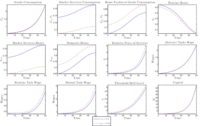
Figure 10 exposes the evolution of the model variable as the productivity of capital increases. On the supply side, as time passes, the price of capital falls which leads to a rise in the capital stock. Since capital becomes cheaper and since it is a substitute to routine hours of work, routine hours of work fall in Europe as in the United States. They are reallocated to the service sector which is composed of the market services sector and the home production sector. Thus, hours worked in manual tasks in both of those sectors increase. We have therefore replicated qualitatively the process of structural transformation which states that as productivity increases resources and thus hours of work are reallocated from the good to the service sector. However, one should notice that in the case of Europe, hours worked in the market service and the good sectors are lower than in the U.S. while domestic hours of work are higher. This is due
to the distortionnary effect of taxation. Indeed, the tax rate is higher by 15% points in Europe than in the U.S. with respect to our calibration. According to our model and our assumptions, households in Europe will choose to reallocate hours worked in the good and the market service sectors to the home production sector in order to avoid as much as possible the distortionnary effect of taxation on their income. It seems that our model allows us to replicate qualitatively the relative deterioration of European labor market outcomes as described in section 2.
5.2
Wages, Prices and Consumption
Since labor demand for market services increases relatively to labor demand for routine tasks, the wage rate for manual tasks increases and eventually exceeds the wage rate for routine tasks; this leads to a rise in the price of market services while the price of goods falls since the price of capital decreases due to productivity growth. Therefore, the relative price of services p increases as in standard multisector growth models described in the introduction. On the demand side, since goods and services are complements, as time passes, both consumption in goods and in market services increase. However, the level of consumption for market services is much lower in the case of Europe due to the high tax rate on labor income. Indeed, as the relative price of market services increases, it becomes more expensive for households to consume market services. Since market services and home produced goods are close substitutes, households will substitute home produced goods for market services.
5.3
Wage Polarization
Figure 11 aims at replicating qualitatively the polarization of wages. As we ex-plained in section 3, wage polarization occurs when the manual to routine wage ratio increases while the abstract to manual wage ratio either remains constant or decreases. The wage ratio between manual and routine tasks increases mono-tonically while the wage ratio between abstract and manual tasks increases and then decreases. Nevertheless, it seems that both lower-tailed and upper-tailed polarizations occur asymptotically since the manual versus routine wage ratio increases while the abstract versus manual wage ratio decreases asymptotically. Taxation doesn’t really have any impact on wage polarization in this model. In-deed, the levels of the wage ratios differ between the United States and Europe. However, what is important is the rate at which they increase and decrease. The rate at which wage ratios vary isn’t affected at all by taxation. Consequently, wage polarization isn’t really affected by taxation. This last observation seems to be compatible with empirical observations. Indeed, the empirical literature observed wage polarization both in Europe and in the United States despite differences in institutions. In our case, we can say that despite differences in labor income tax rates, wage polarization occurs in both entities.
5.4
Share of Hours Worked
Figure 12 presents quantitative results. Indeed, we aim at replicating the share of hours worked in the good and the service sectors. Regarding Europe, the share of services starts at 5.5% of total hours of work; it converges to 9.6%. For
the United States, it starts at 8% and converges to 14.1% of total hours of work. For Europe, the model replicates approximatively the shares in hours of work while for the United States it seems that it overevaluates the evolution of the share of services in total hours of work. Indeed, Europe’s service share increases by almost 6% points in the data while in the model it increases by 4.1% points. For the United States, the service share increases by 1.3% points while the model predicts an increase of 6.1% points. Therefore, the model seems to capture some key mechanisms that drive the evolution of hours worked and their shares at least for Europe. However, there seems to be also other important variables and mechanisms that might drive those variables.
Figure 11: Model - Wage Polarization
S U L TS 33 0 10 20 30 40 50 1 1.5 2 T ime Cg 0 10 20 30 40 50 0.1 0.12 0.14 T ime Cs , Ys 0 10 20 30 40 50 0.65 0.7 0.75 0.8 T ime Ch , Yh 0 10 20 30 40 50 0.1 0.2 0.3 0.4 T ime hr 0 10 20 30 40 50 0.1 0.12 0.14 0.16 Mar ke t Se r v ic e s H our s T ime hms 0 10 20 30 40 50 0.65 0.7 0.75 0.8 0.85 Dome s t ic H our s T ime hmh 0 10 20 30 40 50 1 2 3 4 5 R e lat ive P r ic e of Se r v ic e s T ime p 0 10 20 30 40 50 0.5 1 1.5 2 A bs t r ac t Tas k s Wage T ime Wa g e s 0 10 20 30 40 50 0.5 0.6 0.7 0.8 0.9
R out ine Tas k Wage
T ime Wa g e s 0 10 20 30 40 50 1 2 3 4 5
Manual Tas k Wage
T ime Wa g e s 0 10 20 30 40 50 2 2.5 3 3.5 4 4.5 5 T hr e s hold Sk ill Le ve l T ime η 0 10 20 30 40 50 5 10 15 20 25 30 35 40 C apit al T ime K τU S= 0. 2 τE U= 0. 35
6
Conclusion
As a conclusion, this article aims at deepening our understanding of the process of structural transformation and the phenomenon of labor market polarization. In order to do so, we focused on disaggregated features of hours of work as advised by the literature. Indeed, we studied the role played by productivity growth and taxation in the evolution of hours worked particularly in the low skilled service sector which is the personal service sector according to our sectoral decomposition. In fact, this paper aims at answering the following question: Are productivity growth and taxation accountable for the evolution of low skilled service hours of work?
In order to answer this question, we firstly exposed some stylized facts using the EU KLEMS database of the Groningen Growth and Development Center. We have found that total hours of work decreased in Europe while they increased in the United States. It seems that taxation has played a key role as highlighted by the literature. By looking at more disaggregated data, we have notsed that there has been a process of reallocation of hours worked from the good to the service sectors but hours worked are still lower in Europe in both those sectors. Therefore, we indeed observed the process of structural transformation and the relative deterioration of European labor market outcomes.
Secondly, we built a general equilibrium task model with distortionary taxa-tion and an extra home productaxa-tion sector by following principally the work of Rogerson (2008) and Autor and Dorn (2013). By solving the model numerically, it seems that the model succeeds at replicating some qualitative predictions on the evolution of hours of work, wage polarization, relative prices but also quan-titative predictions on shares of hours worked in the case of Europe. As for the United States, we also succeeded to replicate some major facts but to a smaller extent. However, it seems that we failed to replicate the rise in hours of work in the good sector. Furthermore, the share of the service sector increases sig-nificantly more than in the data. This indicates that productivity growth and taxation are indeed accountable for the evolution of hours of work in the low skilled service sector.
Nevertheless, it also indicates that there must be other key variables and mechanisms that are accountable for the evolution of hours of work. For in-stance, we should focus on mechanisms that explain the rise in hours worked in the good sector in the United States while there has been a decrease for those hours in Europe. The failure of our model to replicate this comes from the fact that the good sector is only subject to one main mechanism i.e. the rise of productivity in capital which reallocates low skilled hours worked from the good sector to the service sector. ICT diffusion might not only drive hours of work away from the good sector. It might also have an impact on education and thus hours of worked by high skilled workers. Moreover, government taxes are used for public expenditures. In our model, we have used lump sum transfers in order to make government spendings neutral. However, the way government resources are used might clearly have an impact on sectoral hours of work. We let those issues to potential future research.
References
[1] Acemoglu, D., & Autor, D. (2010). Skills, Tasks and Technologies: Impli-cations for Employment and Earnings (NBER Working Paper No. 16082). National Bureau of Economic Research, Inc.
[2] Acemoglu, D., & Guerrieri, V. (2008). Capital Deepening and Nonbalanced Economic Growth. Journal of Political Economy, 116(3), 467–498.
[3] Autor, D. H. (2013). The “Task Approach” to Labor Markets: An Overview (NBER Working Paper No. 18711). National Bureau of Economic Research, Inc.
[4] Autor, D. H., & Dorn, D. (2013). The Growth of Low-Skill Service Jobs and the Polarization of the US Labor Market. American Economic Review, 103(5), 1553–97.
[5] Autor, D. H., Katz, L. F., & Kearney, M. S. (2006a). The Polarization of the U.S. Labor Market. American Economic Review, 96(2), 189–194. [6] Autor, D. H., Katz, L. F., & Kearney, M. S. (2006b). The Polarization
of the U.S. Labor Market (NBER Working Paper No. 11986). National Bureau of Economic Research, Inc.
[7] Boppart, T. (2011). Structural change and the Kaldor facts in a growth model with relative price effects and nonGorman preferences (ECON -Working Paper No. 002). Department of Economics - University of Zurich. [8] Cahuc, P., & Zylberberg, A. (2004). Labor Economics (MIT Press Books).
The MIT Press.
[9] Goos, M., Manning, A., & Salomons, A. (2009). Job Polarization in Europe. American Economic Review, 99(2), 58–63.
[10] Kongsamut, P., Rebelo, S., & Xie, D. (1997). Beyond Balanced Growth (CEPR Discussion Paper No. 1693). C.E.P.R. Discussion Papers.
[11] Moreno-Galbis, E., & Sopraseuth, T. (2012). Job Polarization in Aging Economies (Working Paper No. halshs-00856173). HAL.
[12] Ngai, L. R., & Pissarides, C. A. (2007). Trends in Hours and Economic Growth (IZA Discussion Paper No. 2540). Institute for the Study of Labor (IZA).
[13] Ngai, L. R., & Pissarides, C. A. (2008a). Employment Outcomes in the Welfare State (CEP Discussion Paper No. dp0856). Centre for Economic Performance, LSE.
[14] Ohanian, L., Raffo, A., & Rogerson, R. (2008). Long-term changes in labor supply and taxes: Evidence from OECD countries, 1956-2004. Journal of Monetary Economics, 55(8), 1353–1362.
[15] Piketty, T. (1998). L’emploi dans les services en France et aux États-Unis : une analyse structurelle sur longue période. Économie et Statistique, 318(1), 73–99.
[16] Pissarides, C. A. (2007). Unemployment And Hours Of Work: The North Atlantic Divide Revisited. International Economic Review, 48(1), 1–36. [17] Prescott, E. C. (2004). Why do Americans work so much more than
Euro-peans? Quarterly Review, (Jul), 2–13.
[18] Rogerson, R. (2006). Understanding Differences in Hours Worked. Review of Economic Dynamics, 9(3), 365–409.
[19] Rogerson, R. (2007). Structural Transformation and the Deterioration of European Labor Market Outcomes (NBER Working Paper No. 12889). National Bureau of Economic Research, Inc.
[20] Rogerson, R. (2008). Structural Transformation and the Deterioration of European Labor Market Outcomes. Journal of Political Economy, 116(2), 235–259.