Spatial resolution of prism-based surface plasmon resonance microscopy

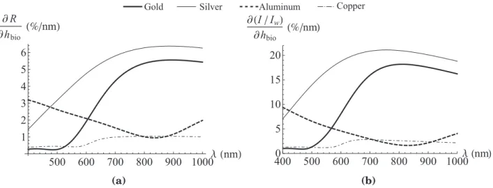
As seen in the Figure S7, with the experimental layer thicknesses (d 2 = 2.4 nm for Cr and d 2 = 3.6 nm for Ti), both theoretical sensitivities are similar reinforcing the validity

The main ad- vantage of our approach is that using a (continuous time) stochastic logic and the PRISM model checker, we can perform quantitative analysis of queries such as if

Dans le cas de notre étude, aucun événement connu ne permet de suspecter une surchauffe postérieure à la formation des inclusions, qui de plus ne présentent aucune

Prismatic adaptation modulates line bisection performance in both healthy individuals and patients and we suggest that LPA likely modulates the left PPC-M1 functional connectivity

For the last goal to analyze the importance of individual reaction on downstream signaling molecules, we compute the steady state probabilities of Akt and MEK12 in 31 different

The current testing method such as the vicat needle for cement paste and penetration resistance test for concrete methods measure at intervals.These methods can be applied before

To distinguish between existing collaborative mechanisms that are supporting agro- ecological transitions in the Global South, we have adopted two criteria pertaining to the

In this article we analyze the links between the spatial distribution of cashew-nut farming, which is a new agricultural product in southern Burkina Faso, and the