Macro-continuous dynamics for hyper-redundant robots: application to locomotion bio-inspired by elongated animals

HAL Id: hal-00761258

https://hal.archives-ouvertes.fr/hal-00761258

Submitted on 5 Dec 2012

HAL is a multi-disciplinary open access

archive for the deposit and dissemination of

sci-entific research documents, whether they are

pub-lished or not. The documents may come from

teaching and research institutions in France or

abroad, or from public or private research centers.

L’archive ouverte pluridisciplinaire HAL, est

destinée au dépôt et à la diffusion de documents

scientifiques de niveau recherche, publiés ou non,

émanant des établissements d’enseignement et de

recherche français ou étrangers, des laboratoires

publics ou privés.

application to locomotion bio-inspired by elongated

animals

Frédéric Boyer, Shaukat Ali, Mathieu Porez

To cite this version:

Frédéric Boyer, Shaukat Ali, Mathieu Porez. Macro-continuous dynamics for hyper-redundant robots:

application to locomotion bio-inspired by elongated animals. IEEE Transactions on Robotics, IEEE,

2012, 28, pp.303 - 317. �hal-00761258�

Macro-Continuous Dynamics For Hyper-Redundant

Robots: Application to Kinematic Locomotion

Bio-Inspired by Elongated body Animals

Frédéric Boyer, Shaukat Ali, and Mathieu Porez

Abstract—This article presents a unified dynamic modeling

approach of (elongated body) continuum robots. The robot is modeled as a geometrically exact beam continuously actuated through an active strain law. Once included into the geometric mechanics of locomotion, the approach applies to any hyper-redundant or continuous robot devoted to manipulation and/or locomotion. Furthermore, exploiting the nature of the resulting model as being a continuous version of the Newton-Euler model of discrete robots, an algorithm is proposed which is capable of computing the internal control torques (and/or forces) as well as the rigid net motions of the robot. In general, this algorithm requires a model of the external forces (responsible for the self propulsion), but we will see how such a model can be replaced by a kinematic model of a combination of contacts related to terrestrial locomotion. Finally, in this case, that we name "kinematic locomotion", the algorithm is illustrated through many examples directly related to elongated body animals such as snakes, worms or caterpillars and their associated bio-mimetic artifacts.

Index Terms—Beam theory, bio-inspired locomotion,

contin-uum robots, geometric mechanics, hyper-redundant robots, kine-matic constraints, Newton-Euler dynamics.

I. INTRODUCTION

Engineers have always been inspired by nature. In the beginning of robotics, robots resembling to human arm were designed using discrete mechanisms devoted to the manip-ulation tasks of industrial manufacturing processes. These discrete mechanisms consist of serial chains of rigid bodies connected by lumped degrees of freedom (DoFs) and are today included into the wider class of multibody systems. With the passage of time, the researchers in this field started developing mechanisms with more and more DoFs, thus introducing a new generation of robots called as hyper-redundant robots (HRRs) since they may be considered as having an infinite degree of redundancy with respect to the six dimensional task consisting of moving a rigid body in space. In case of locomotion, these systems are usually inspired by vertebrate elongated body animals such as snakes [1] and anguilliform fish [2], where the vertebrae correspond to the rigid bodies of the associated multibody system. From this point of view, these animals can be effectively considered as continuous, the Manuscript received Month Day, Year; revised Month Day, Year. The associate editor coordinating the review of this paper and approving it for publication was ...

The authors’ are with the Ecole des Mines de Nantes, Nantes, France. (email: frederic.boyer@mines-nantes.fr, shaukat.ali@mines-nantes.fr, mathieu.porez@mines-nantes.fr)

Publisher Item Identifier .

european eel having more than 130 vertebrae, while some

species of big snakes have more than500. Nowadays, thanks to

the research on bio-mimetic robots, the concepts of continuum robots and soft-bodied robots are extending robotics even further. In fact, unlike traditional robots, these robots, inspired by the invertebrate organisms known as muscular-hydrostats, do not contain any rigid organs. Also, their shape changes are continuous along their body length similar to that of an elephant trunk [3], the mammalian tongue [4], caterpillars [5], earthworms [6], octopus arms [7] etc. Finally, all these systems today form the general class of continuous-like robots. Regarding their potential impact, let us first note that using the same single chain morphology, elongated body continuous like robots would offer a wide spectrum of applications ranging from manipulation to locomotion on earth as well as in water. Moreover, once connected to a discrete mechanism, they could be used as versatile manipulators as well as grippers. Finally, due to their slender morphology, they could play a crucial role to achieve rescue missions in unstructured, highly cluttered and confined environments e.g. collapsed buildings, narrow spaces etc.

With the progress of these researches, the extension of the basic robot models (geometric, kinematic and dynamic mod-els) to these new systems became a crucial step towards their future success. Regarding this point, several researchers have done extensive work related to HRRs or continuous robots in order to investigate the usual problems of robotics such as motion planning, gait generation, kinematic and dynamic modeling, design and control etc. We refer the reader to [8] which surveys the state of the art on soft robotics. Historically, the initiative was undoubtedly taken by Hirose through his pioneering work related to the design and control of snake-like devices [1].

Based on these seminal works, many contributions to kine-matic modeling have been proposed [3], [9]–[12]. Concerning dynamics of continuum robots, a few works on this topic have been proposed [13]–[16]. In fact, the existing approaches can be categorized into two main sets depending on whether the robot is considered as a multibody system with a large number of DoFs [17], [18], or directly as a continuous deformable medium. In the first case, the modeling is facilitated by the fact that mathematical tools from usual discrete robotics are already available. On the other hand, adopting a continuous model from the beginning can greatly facilitate the formula-tion, analysis and resolution of the robotics problems related to manipulation [15], [19] and locomotion [1], [10], [20].

However, applying this second type of approach necessitates giving a material reality to the continuum kinematics. For instance, the backbone curves of references [9], [10] have to be completed with a material lateral extension enabling the inertia of the robot to be defined as achieved in [15], [19] for planar robots. Alternatively, the Geometrically Exact Beam Theory (GEBT) of J.C. Simo [21], [22] has been used for the modeling of passive steerable needles in the context of medical robotics [23],[24], while in [8] and [25], it has been applied to the real soft robot OctArm [26]. In the GEBT, a beam is modeled as a one dimensional Cosserat medium [27], i.e. a multibody system made of an infinite number of rigid bodies, or cross sections, of infinitesimal length assembled along the line of their centroids, each cross section being able to move with respect to the others due to some strain time-variations. Starting from this point of view, in [2] a continuous eel-like robot is modeled as a strain (curvature) - actuated ge-ometrically exact beam. Pursuing a macroscopic modeling approach, each Cosserat cross section of the actuated beam mimics a vertebra of the animal (here the eel), while the imposed strain law models the actuated infinitesimal joints of the corresponding continuous rigid robot. Once related to the general theory of locomotion on principal fiber bundles [28], such a model can be used to solve the following two problems both using the curvature time law as control input: 1) compute the control internal torques (and/or forces), i.e. solve the inverse torque dynamics. 2) compute the net motion of a reference cross section (for instance attached to the head) propelled by the external forces exerted by the surroundings (i.e., solve the forward locomotion dynamics). The approach was termed macro-continuous since, like the Variable Geom-etry Truss evoked in [19], it is suitable for modeling hyper-redundant robots at a macroscopic scale where they can be approximated as a beam. It is naturally adapted to the highest levels of the mechanical design as well as the generation of complex gaits involving a lot of DoFs as this is usually the case of HRRs [20].

In the article here presented, we reconsider this approach for locomotion and extend it to cases where: 1) The configuration space of the cross sections is an arbitrary Lie group. 2) The control strain law is arbitrary (curvature, twist, stretching...). 3) The external forces responsible for the propulsion are not forced to be those produced by a fluid but can be imposed by the contact with the ground and modeled through kinematic constraints.

In this case, like discrete multibody systems [29], when the number of independent constraints is larger than the number of net motions DoFs, the locomotion dynamics are replaced by a kinematic model entirely governed by the constraints. Geomet-rically, these forward locomotion kinematics are nothing but a continuous version of the finite-dimensional kinematic connec-tions of nonholonomic mechanics [28], [30]. As a consequence and contrary to the case of eel swimming, the locomotion dynamics are not required to deduce the net motions but are used in their inverse form to compute the resultant and moment of external forces produced by the contacts. Once these elements are computed, they are distributed on the contacts in order to fix a possible set of external reaction

forces and couples which are used in a second step by the algorithm to compute the internal actuation torques and/or forces. Finally, the kinematic constraints are deduced from the model of a few types of contacts, which will allow us to apply the macro-continuous approach to terrestrial locomotion of several elongated body animals as earthworms (crawling worm), inchworms (measuring caterpillars), snakes in planar and three-dimensional lateral undulations.

This article is structured as follows. In section II, we take an in-depth look at the parametrization of GEBT particularly, the strain field definitions and their relation to discrete joint kinematics. Section III presents a comparative study of the beam kinematics and HRRs. Based upon the parametrization of section II, the continuous kinematic and dynamic models are stated in section IV. In section V, the continuous Newton-Euler computed-torque algorithm of [2] is presented in a more general context. In section VI, the common types of terrestrial contacts are modeled as kinematic constraints. Based upon the model of contact, a modified algorithm is developed in section VII. Finally, in section VIII the proposed approach is illustrated by examples related to terrestrial locomotion robots bio-inspired by elongated body animals.

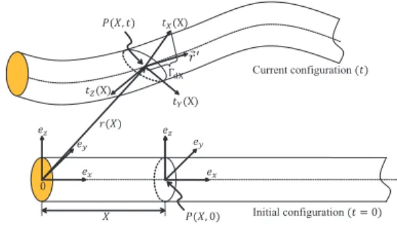
Initial configuration Current configuration

Fig. 1. Frames and parametrization

II. BASIC NOTATIONS AND DEFINITIONS

In the subsequent sections, we use the language of geomet-ric mechanics [31] as this has already been adopted by [2], [23], [32] in the context of continuum robots. In this regard, G ⊆ SE(3) is a n dimensional Lie group of transformations of the ambient space provided with an orthonormal fixed frame

Fs= (O, ex, ey, ez). The Lie algebra of G is denoted by g and

defined as the space of infinitesimal transformations or twists,

i.e. the tangent space to G at g = 1 endowed with the Lie

bracket[, ]. Introducing the internal product on g, we define g∗

, the vector space of 1 forms on g, or wrenches. Differentiating

the group automorphismh ∈ G #→ ghg−1 _{ath = 1, gives the}

action map Adg of G on g. Then differentiating Adg with

respect to g at g = 1 defines the adjoint map ad(.) of g

on g. Dualizing ad(.) defines the co-adjoint map of g on g∗

whileAd∗

(.) is the co-action ofG on g

∗

. See Appendix A for more usual definition of these operators as well as their matrix

expressions in SE(3).

For any vector V ∈ R3_{, V}∧

(or ˆV ) denotes the

V∧ ₌ ! ˆ ω v 0 0 " , where ω ∈ R3 _{and ( ˆV )}∨ _{= V . In}

agreement with [2], a hyper-redundant robot may be modeled

by a Cosserat beam in finite 3D transformations and small

strains with the backbone curve of the robot assimilated to the beam centroidal line. In this approach, each cross section

of the beam (of length l), supposed rigid, is labeled by its

abscissa X in the initial configuration in which the beam is

straight and aligned on (O, ex) (see Fig. 1). At any rigid

cross section X, a mobile orthonormal frame is attached

t #→ Fm(X, t) = (P, tX, tY, tZ)(X, t) whose origin P (X)

and the first vector tX(X) coincide with the center of the

cross section and its unit normal vector, respectively. With this choice, the configuration of any mobile frame is defined by the

action of an element ofg ∈ SE(3) applied to the fixed frame

Fs. It thus becomes possible to introduce the first definition of

the robot configuration space as a functional space of curves

inSE(3), parameterized by the material abscissa, i.e.:

C1= {g : ∀X ∈ [0, l] #→ g(X) ∈ SE(3)}. (1)

Later, we will introduce a second definition of configuration space as a principal fiber bundle. The derivative operators ∂(.)/∂X and ∂(.)/∂t will be indicated as a "prime" and a "dot", respectively. On the robot, two vector fields are defined

inse(3). The first is the time-twist field:

ˆ

η : X ∈ [0, l] #→ ˆη(X, t) = g−1˙g ∈ se(3), (2)

where η(X, t) defines the infinitesimal transformation

under-gone by the cross section X between two infinitely close

instantst and t + dt. The second is the space-twist field such

that: ˆ

ξ : X ∈ [0, l] #→ ˆξ(X, t) = g−1g%

∈ se(3), (3)

where ξ(X, t) defines the infinitesimal transformation

un-dergone by the cross section X at fixed time t when the

material axis slides from X to X + dX. Now depending

on the considered robot, certain degrees of freedom between any two contiguous cross sections are actuated while others are constrained to constant values through the design of internal joints (that are assumed ideal). Mathematically, this

corresponds to identify ˆξ to a desired control field explicitly

dependent on the time and noted ˆξd(t), i.e.:

ξ(X) = ξd(X, t), ∀(X, t) ∈ [0, l] × R+. (4)

Finally, ξd parameterizes the internal kinematics of the robot,

i.e. the continuous infinitesimal homologous of the usual internal joints of discrete multibody systems.

III. BEAM-KINEMATICS ANDHRRS

We now list the different possible actuations of ξ and

comment their relations to continuum robotics and beam theory. For this, we start from definition (4) which we detail as follows: g−1_g% = ! RT_R% _RT_r% 0 0 " = ! # Kd(t) Γd(t) 0 0 " = #ξd(t), (5) where Kd = (KdX, KdY, KdZ) and Γd = (ΓdX, ΓdY, ΓdZ).

The components of these two vectors have the following

meanings: KdX is the rate of twist per unit of material

beam length while KdY and KdZ represent the curvatures

of its centroidal line in the planes(P, tX, tZ) and (P, tX, tY)

respectively. In the same way,ΓdX− 1 is the rate of stretching

of the centroidal line (see Fig. 1) whileΓdY andΓdZ are the

local transverse shearing rotations around the axes(P, tZ) and

(P, tY) respectively. Now, depending on whether these scalar

strain fields are actuated or not, different cases, relevant to robotics, are possible, from that where the internal kinematics are the most actuated to where they are the least actuated as summarized in table I:

TABLE I

ACTUATEDDOFS VSBEAM THEORY

Case Constraints DoFs Beam Theory Remarks

1 No constraints 06 Timoshenko-Reissner Full actuated beam 2 ΓdY = ΓdZ= 0 04 Extensible Kirchoff Cross sections stay perpendicular to vertebral axis 3 Case 2 with ΓdX= 1 03 Inextensible Kirchoff infinitesimal ver-sion of a spheri-cal joint 4 Case 3 with KdX= 0 02 No corresponding beam In passive beams, 3D bending always produce torsion 5 Case 4 with KdY = 0 01 Inextensible planar Kirchoff

Planar case with Yaw DoF actua-tion

Remarks:

• Each of these internal DoFs finds an application in nature

for elongated body animals’ locomotion. In fact, one of

the two curvaturesKY andKZ actuates the yaw in the

plane of propulsion, while the other actuates the pitch for

complex3D maneuvers involving the body. The torsion

KXhas a direct action on the roll whose control is crucial

to stabilize the orientation of the head of robots

bio-inspired by eels for instance. As for linear DoFs, ΓX

actuates the traction-compression as used by large snakes

whileΓY andΓZcan be actuated through the movements

of the skin and scales with respect to the backbone.

• A similar relation to (5) exists in the case of any

sub-group ofSE(3). Also, in the following, we will consider

(5) withg belonging to any subgroup G of SE(3) of Lie

algebra g.

IV. THE CONTINUOUS MODEL OFHRRS

From now on,go, ˙go and ¨go denote the position, velocity

and acceleration of the cross sectionX = 0 on G, respectively.

The continuous dynamic model of a HRR splits into 5 sub-models detailed in the following subsections.

A. Continuous model of transformations

This is immediately derived from definition (5) of internal DoFs:

g%

= g ˆξd(t), (6)

B. Continuous model of velocities

By taking derivative of (2) with respect to space (i.e. X),

and by invoking (5), we obtain:

η%= −adξd(t)(η) + ˙ξd(t), (7)

with boundary conditions:η(X = 0) = ηo= (g−1o ˙go)∨.

C. Continuous model of accelerations

This is inferred by taking derivative of the previous model (7) with respect to time:

˙η%= −adξd(t)( ˙η) − ad_ξ˙d(t)(η) + ¨ξd(t), (8) whose solutions are fixed by the boundary conditions:

˙η(X = 0) = ˙ηo= (g−1o g¨o− go−1˙gogo−1˙go)∨.

Remark 3: On reconsidering the continuous kinematic model (6), it becomes clear that it is always possible to reconstruct the configuration of the beam from the knowledge

ofgoand that of the strain fieldξd. Thus, a second definition of

the configuration space of a robot can be given as the principal fiber bundle:

C2= G × S, (9)

whereG stands for the configuration of the head frame, while

S is the shape space here defined as the following functional space of curves in the Lie algebra:

S = {ξ : ∀X ∈ [0, l] #→ ξ(X) ∈ g}. (10)

In this second definition of the robot configuration space, the

cross section X = 0 plays the role of reference body, i.e.

a body whose motion defines the reference of rigid overall motions with respect to which the shape deformations are measured. In bio-mimetics, this reference body is usually attached to the head of the bio-inspired robot.

D. Dynamics onC1: continuous model of the internal torques

By applying on C1the Hamilton principle for a continuum

robot subject to a density of imposed external wrenches per

unit of beam length F on ]0, l[ and two punctual external

wrenches F− and F+ imposed on X = 0 and X = l

respectively, one obtains the following Partial Differential Equations (PDE) [33]: ∂ ∂t ! ∂L ∂η " − ad∗ η ! ∂L ∂η " + ∂ ∂X ! ∂L ∂ξ " − ad∗ ξ ! ∂L ∂ξ " = F , (11) whose solutions are fixed at each instant by the boundary conditions:

∂L

∂ξ(0) = −F− , and:

∂L

∂ξ(l) = F+, (12)

where the Lagrangian density of a continuum robot has been

defined by L= T−U = (1/2)(ηT_(Mη)−ΛT_(ξ−ξ

d(t)), with:

M ∈ g∗

⊗ g, the inertia tensor density, and ∂U/∂ξ = Λ ∈ g∗

, the density of internal wrenches ensuring the forcing of the

Lagrangian internal kinematic constraints: ξ = ξd(t). Let us

note here thatΛ is a field of Lagrange multipliers and that, for

the actuated internal DoFs, the associated multipliers are forces

or/and torques exerted by the actuators while for the passive DoFs, the multipliers are internal reaction torques or forces. Note also that with such a choice, the internal kinematics are assumed to be inelastic and the robot turns out to be a

continuous rigid robot1_{. Now, if we note ∂T/∂η = Mη the}

density of kinetic wrench along the robot, we find:

M ˙η − ad∗

η(Mη) − Λ

%

+ ad∗

ξd(t)(Λ) = F , (13)

with boundary conditions:

atX = 0: Λ(0) = −F− and atX = l: Λ(l) = F+. (14)

Finally, (13) and (14) are considered in the following as the dynamics of the internal wrenches or more simply as the "internal dynamics".

E. Dynamics onC2: dynamics of the reference body

The dynamics onC2are derived from those onC1by forcing

the virtual and real velocity fields in the Hamilton principle (which previously led to (13-14)) to verify the following constraint:

η = Adk(ηo), (15)

where, k = g−1_g

o. Note that, the defined field (15) is simply

the time-twist field on the beam induced by the movement of the head alone, while the body is frozen in its current shape. In these conditions, the internal wrenches do not work in such a field and the balance of virtual work reduces to:

$ l 0 Ad∗k(M ˙η − ad ∗ η(Mη) − F )dX = Ad ∗ k+F+− F−, (16)

where ˙η is replaced by the acceleration field compatible with

(15), i.e.:

˙η = Adk( ˙ηo) + adη(Adk(ηo)) + Adk(ηo2) − (Adk(ηo))2

= Adk( ˙ηo) + ζ, (17)

which defines ζ(X) as the material (or body) acceleration of

cross section X induced by the body shape motion and the

movement of the head except for its pure acceleration (i.e. ˙ηo).

Finally, when the calculations are done and the kinematic

reconstruction equation ˙go = goηˆo is taken into account, the

dynamic equations onC2 can be written as:

! ˙ηo ˙go " = ! M−1 o (ξd)Fo(ξd, ˙ξd, ¨ξd, go, ηo) goηˆo " , (18)

with:Fo = Fin+ Fext, and where we introduced the inertia

tensor of the whole robot reduced to the reference cross section

i.e. inX = 0: Mo= $ l 0 Ad∗ kMAdkdX, (19)

as well as the external wrenches, reduced to the reference cross section: Fext= −F−+ Ad∗_k +F++ $ l 0 Ad∗ k(F )dX, (20)

1_{Alternatively, the model of internal dynamics can be enriched by adding} elastic and viscous terms in U

and the inertial wrenches reduced to the reference cross section: Fin= − $ l 0 Ad∗ k(Mζ − ad ∗ η(Mη))dX. (21)

In the following, (18) will be considered as the dynamics of the reference body net motions controlled by the shape time variations, i.e. the "locomotion dynamics".

V. DYNAMICALGORITHM OF THECONTINUUMROBOTS

By defining the kinematic state vector X1 = (g, η, ˙η), the

kinematic models (6,7,8) can be easily grouped together into a single spatial Ordinary Differential Equation (ODE):

X%

1= f1(X1, ξd(t), ˙ξd(t), ¨ξd(t)). (22)

Similarly, the internal dynamics (13) can be stated in the form

of the following spatial ODE, of the state vectorX2= (X1, Λ):

X% 2= f2(X2, ξd(t), ˙ξd(t), ¨ξd(t)), (23) with:f2= ! f1 ad∗ ξd(t)(Λ) + M ˙η − ad ∗ η(Mη) − F " . (24) Then, the terms appearing in the locomotion dynamics (18) can also be calculated by spatial integration of a single ODE

of the state vector X3= (X1, Mo, Fo):

X% 3= f3(X3, ξd(t), ˙ξd(t), ¨ξd(t)), (25) with:f3=   Ad∗f1 kMAdk Ad∗ k(ad ∗ η(Mη) + F − M ˙η)   , (26)

where theζ of (21) can be replaced by ˙η in (26) if the initial

spatial conditions of (25) verify ˙η(X = 0) = ˙ηo= 0. In fact,

in this case (17) shows thatζ = ˙η all along the beam. Finally,

as we will now see, in every case the algorithm integrates (25) in these conditions, so that (26) makes sense.

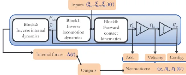
All the above ODEs form a general algorithm as shown in

Outputs

Acc. Velocity Config. Internal forces Inputs: Block2: Inverse internal dynamics Block1: Forward locomotion dynamics Net motions: (ξ ξ ξd,! !!d, d)( )t ( )t Λ (go,η η!o, o)( )t o g o η o η! ∫ ∫

Fig. 2. General algorithm of HRRs

Fig. 2 to solve the dynamics of a HRR. The execution of algorithm is summarized as follows:

1) In block 1, integrate the spatial ODE (25) fromX = 0 to

X = l initialized by X3(0) = (go, ηo, 0, 0, F−), to give

Mo andFo.

2) In block 1, calculate ˙ηo and then integrate (18) between

t and t + ∆t in order to deduce the new reference state

(for the following time-step):(go, ηo)(t + ∆t)

3) In block 2, integrate the spatial ODE (23) fromX = 0

toX = l initialized by X2(0) = (go, ηo, ˙ηo, F−) to give

Λ (and F+ by way of verification).

Remarks:

• Let us remark that the above algorithm is nothing else

but a continuous version of the Newton-Euler discrete algorithm of mobile multibody systems of [29], where (22) stands for the forward recursive kinematics, (23), for the backward recursive computation of inter-body wrenches, and (25) stands for the recursive computation of the locomotion dynamics.

• The algorithm solves the forward dynamics by computing

the net (reference) acceleration from a model of the external forces. In general, such a model can be very complex as in the case of swimming in which, in the ab-solute, it requires to integrate the Navier-Stokes equations of the surrounding flow [34]. In the case of terrestrial locomotion, the above algorithm can be used with exter-nal forces modeled as physical laws, e.g. friction laws. However, for the sake of simplicity of analysis, it can be useful to consider the contacts as ideal. In this case, they can be modeled as constraints instead of forces as discussed in the following section. In the next step, we will see that when the number of constraints is sufficient, locomotion dynamics can be replaced by kinematics and the locomotion is named as "kinematic locomotion".

VI. KINEMATIC MODELING OF CONTACTS

In this work, we consider two types of contacts: anchorages and supports. Anchorages are modeled as bilateral holonomic constraints while supports are modeled as non-holonomic constraints. In both cases the contacts are distributed along the body axis. In the case of anchorages, two types are envisaged: either the anchorage is fixed on the material axis of the robot

on an abscissa, noted C, constant in relation to time or, in

contrast, this abscissa, notedC(t), is explicitly dependent on

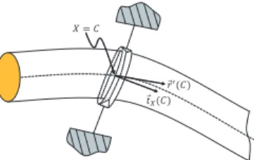
time. The former is known as a locked anchorage and the latter is a sweeping anchorage. Concerning supports, the contact is always sweeping, as the robot can slide freely thanks to an annular type contact (see Fig. 3). Anchorages and supports are assumed to be attached to rigid bodies submitted to imposed relative motions in the fixed earth frame. Finally, as we will

Fig. 3. Annular contact (CSFS)

practical interest for modeling numerous locomotion modes as illustrated in table II.

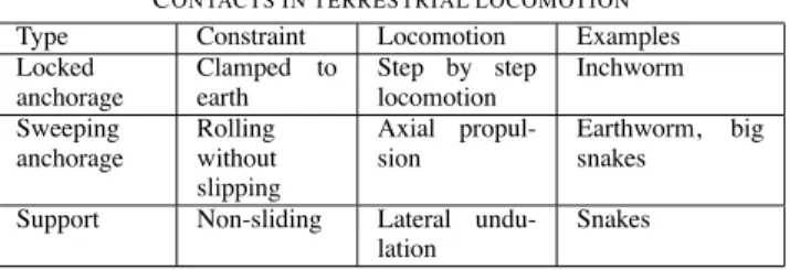
TABLE II

CONTACTS IN TERRESTRIAL LOCOMOTION

Type Constraint Locomotion Examples

Locked anchorage Clamped to earth Step by step locomotion Inchworm Sweeping anchorage Rolling without slipping Axial propul-sion Earthworm, big snakes

Support Non-sliding Lateral

undu-lation

Snakes

A. Anchorages

For a locked anchorage as shown in Fig. 4(a), where the

robot is anchored at a fixed material pointC ∈ [0, l], we write

the geometric model as:

g(C) = gc(t), (27)

(a) (b)

Fig. 4. (a) Locked anchorage; (b) Sweeping anchorage

where t #→ gc(t) denotes a function of time in G which

represents the imposed motion of the anchored rigid body.

In particular, if gc is independent of time, then this body

is fixed, as in the case of a manipulator robot anchored in the ground or more simply a cantilevered beam (see Fig. 4(a)). For a sweeping anchorage as shown in Fig. 4(b)), the geometric model of contact cannot distinguish it from a locked

anchorage, both considered at the same instant t. In fact, in

the second case, we still have:

g(C(t)) = gc(t), (28)

which coincides with (27) when C = C(t). In contrast,

the kinematic model can make the distinction since, for the sweeping anchorage, by taking total derivative with respect to

time (denoted asd(.)/dt) of (28):

d

dtg(C(t)) = ˙g(C(t)) + g

%

(C(t)) ˙C(t) = ˙gc(t), (29)

which is multiplied by g−1_{(C(t)) to obtain, invoking (28)}

again, the sweeping anchorage constraints in g:

η(C(t)) + ξd(C(t), t) ˙C(t) = ηc(t), (30)

where ηc(t) = (gc−1˙gc)∨(t), (ηc(t) = (VcX, VcY, VcZ,

ΩcX, ΩcY, ΩcZ)T(t), when G = SE(3)) is the time-twist

imposed on the rigid body supporting the anchorage and where (30) allows one to recover the kinematic form of a locked

anchorage:η(C) = ηc(t) when C is time-independent. Finally,

let us note that (30) produces a set of dim(g) independent

scalar constraints.

B. Supports

Before describing the details of their modeling, let us recall that supports are sweeping by nature so they can only be accounted for by kinematic constraints. Here, we consider supports named as Cross Sectional Follower Supports (CSFS). Such supports follow the cross sections in their lateral motions (see Fig. 3). A CSFS is an annular joint preventing all relative translation velocities (of the beam with respect to the support)

in the plane of a given cross section of abscissa X = C.

Thus, for a movement in the space R3(i.e.G = SE(3)), such

a contact exerted in anyC ∈ [0, l] is modeled by the relations:

( ˙r(C) − ˙rc(t)) × tX(C) = 0 , (ω(C) − ωc(t))TtX(C) = 0

(31)

where ω(X) = ( ˙RRT₎∨_{(X) denotes the spatial angular}

velocity of the X-cross-section while ( ˙rT

c, ωcT)T(t) is the

spatial twist imposed on the rigid support. After computation, (31) leads to the following three non-holonomic constraints

VY(C) = VcY(t), VZ(C) = VcZ(t), ΩX(C) = ΩcX(t),

(32)

whereVcY(t), VcZ(t) are the lateral velocities expressed in

the cross section frame whileΩcX(t) is the axial component

of the angular velocities. All of them being imposed on the

C-cross-section by the movement of the obstacle, these velocities

are null if the obstacle in question is fixed. Finally,C can itself

move along the material robot axis following a time law of the general form:

˙

C = VcX(t) − VX(C), (33)

where VcX is imposed by the axial motion of the support

while VX(C) is ruled by the locomotion. Lastly, let us note

that when the given support follows the cross section not only

laterally but also axially, then ˙C = VcX(t) − VX(C) = 0.

C. Models of contact forces

As the contacts are ideal, the reaction (contact) forces are identified as Lagrange multipliers associated to the scalar

constraints taken from (30) and (32). When G = SE(3), an

anchorage introduces six multipliers (i.e. the six components of a complete reaction wrench) while a support transmits two lateral forces and one axial torque for a three-dimensional movement and only one lateral force for a planar motion. When the anchorages and/or the supports are imposed at the ends, the reaction forces associated with them enter into the calculation of the dynamics via a contact component of

the apical external wrenches F± that we note Fc,± (where

"c" means "contact"). As long as the contacts are defined

inside the domain of the beam, i.e. if C ∈]0, l[, then each

of them adds a set of kinematic constraints in g and an

associated reaction wrench (defined in g∗), that enters into

the model via F which then contains a contact term of

the form: Fc(C)δ(X − C), where δ denotes the Dirac

distribution. Finally, according to (20), any distribution of

contacts produces a contribution to Fext which is noted Fc

VII. ALGORITHM IN KINEMATIC CASE

When the number of constraints (imposed by the contacts)

is equal or higher than the dimension of the fiber of C2, the

system is said fully or over constrained and the net motions are entirely ruled by the kinematic model of the contacts which takes the most general explicit form:

˙go= goηˆo= gof (gˆ o, ξd(t), ξd%(t), ξ %%

d(t), ..., ˙ξd(t)), (34)

where the model of reference accelerations can be obtained

by simple time differentiation of f . In this case, the

locomo-tion is called "kinematic locomolocomo-tion" (to distinguish it from the previous dynamic locomotion case) and the locomotion dynamics (18) are used in their inverse form to calculate the contact wrench induced by the external constraints, i.e.:

Fc= Mo˙ηo− Fin− Fother, (35)

whereFother, denotes the contribution toFextbrought by the

distribution of external forces of other origin than contact.

Such a distribution will be denoted by(Fother,±, Fother) and

models external loads as gravity, pressure and viscous forces etc.

Outputs

Acc. Velocity Config. Internal forces Block2: Inverse internal dynamics Block1: Inverse locomotion dynamics Net motions: ( )t Λ (go,η η!o, o)( )t o g o η o η! _{∫ ∫} Block0: Forward contact kinematics , c c F F ± Inputs:(ξ ξ ξd,! !!d, d)( )t

Fig. 5. Algorithm of a HRR with kinematic constraint model

Going further, when the number of constraints is strictly

higher than the dimension of the fiber of C2, the overall

motions of the robot are over-constrained which means that:1)

the internal movements must be compatible2_{,2) the reaction}

unknowns Fc,± and Fc are under-determined as they are

only required to verify the locomotion dynamics (35). Finally, taking these considerations into account, the new constrained algorithm as shown in Fig. 5 can be summarized as follows:

1) In Block0, calculate (ηo, ˙ηo) from a kinematic model of

contacts of the form (34) and its time derivative, and

integrateηobetweent and t + ∆t in order to deduce the

new configuration of the reference cross section (for the

following time-step):go(t + ∆t).

2) In Block1, integrate the spatial ODE (25) fromX = 0 to

X = l initialized by X3(0) = (go, ηo, 0, 0, Fother,−) and

withF = Fother, to giveMo,Fin,Fother(andFother,+

by way of verification).

3) In Block1, calculate thanks to (35), the resultant of the

reaction wrenchesFc induced by the contacts.

2_{with the risk, if this is not the case of preventing mobility and, due} to the hyper-statism, of producing internal stress resolved by replacing the constraints induced by the internal joints, assumed ideal, by rheological passive laws.

4) After a distribution3 _{of F}

c at the p contact points

Ci=1,..p, integrate in Block2 the spatial ODE (23)

subjected to the distribution of reaction wrenches (Fc,±, Fci) applied at the contact points, and initialized

by X2(0) = (go, ηo, ˙ηo, F−) to calculate the internal

wrenchesΛ.

Remarks:

• In the following we do not specify the form of the

loco-motion kinematics beyond its expression (34), preferring to investigate it, case by case, for particular examples.

Let us just say here that the function f in (34) must be

calculated fromf1of (22) and from considerations related

to the way of locomotion studied (particularly based on biological observation) as well as the contact model as introduced in section VI.

• Hyper-redundant manipulators can be considered as a

subclass of fully constrained case. In fact here, the

reference cross section X = 0 is clamped in a rigid

basis enduring an imposed motion (in particular, null)

defined by X1(0) = (go, ηo, ˙ηo)(t). In this case, steps 1,

2 and 3 of the above algorithm can be avoided. Indeed, the reference motions require no calculations as they are known by their time laws.

• Note that if f is linear in ˙ξ_d and independent of g_o,

the kinematic model under the constraints of contacts defines a principal kinematic connection on the principal

fiber bundle C2, i.e. a continuous version of the discrete

connections studied in the mechanics of non-holonomic systems [30].

VIII. ILLUSTRATIVE EXAMPLES

We now consider several examples of terrestrial locomotion where the net motions are ruled by kinematic locomotion deduced from the model of contacts summarized in table II.

A. burrowing worm in 1D

(a)

Anchorage

(b)

Fig. 6. (a) Initial reference configuration; (b) Deformed configuration

This is a burrowing robot inspired by earthworms. The earthworm is assumed to have a homogenous volumetric mass ρ. Based on biological knowledge [35], the radial dilation of the cross sections caused by axial compression ensures the worm’s anchorage in its surroundings: a tunnel burrowed by prior digestion of the earth in front of the head. Locally, the radial anchorage is achieved by rigid setae which push into the earth radially when the cross section is at maximal dilation (see Fig. 6(b)). The beam model is that of a rod actuated

3_{Univocal if the number of constraints equal the dimension of the fiber,} multivocal, if it is higher.

in traction-compression. The forward gait is produced by a backward wave of traction-compression of the form:

ΓdX(X, t) = 1 + ǫ sin(ω(t − X/c)). (36)

The dilation (striction) of the cross sections is controlled by the traction by adding to the Cosserat theory presented earlier the axial volume preservation constraint written as:

A(X, t) = A(X, 0)/ΓdX(X, t), (37)

which is simply derived from: A(X, t)dS = A(X, 0)dX

whereA(X, t) is the area of the cross section X at the instant

t, while dS = ΓdXdX is the length at current t of the part of

the worm of initial lengthdX initially located at X.

In this scenario, the previous general construction applies by

replacing G (as well as g and g∗

) by R identified with the

commutative subgroup of translations along thex-axis (which

also coincides with its Lie algebra and its dual). It follows that the adjoint maps disappear from the expressions and we can

propose more simply g = x, go = xo,η = ˙x, ξd(t) = ΓdX,

F = )i=pi=1nci δ(X − Ci(t)), Λ = n where Ci denotes the

material abscissas of the p anchorage points (see Fig. 6(b))

defined at each instant by the condition of the local maximal contraction:

Ci(t) ∈ [0, l], such that: ΓdX(Ci(t), t) = 1 − ǫ. (38)

With these considerations, the worm’s continuous kinematic model takes the form (22) with:

X% 1= (x % , ˙x% , ¨x% )T _{= (Γ} dX(t), ˙ΓdX(t), ¨ΓdX(t))T, (39)

whose solutions are fixed by the anchorage points. In partic-ular, it should be noted that any cross section anchored to the ground by the setae imposes a constraint on the movement in the fiber, identified here to R. It follows that the net movements are derived from a kinematic model. Such a model can be simply obtained by imposing that, at any anchorage point

Ci(t), the velocity of slipping is null, i.e. Ci(t) represents

a sweeping anchorage point. Also, by invoking the contact

kinematics (30) with C(t) = Ci(t), η(C(t)) = ˙x(Ci(t)),

ξd(t) = ΓdX(t), and ηc(t) = 0 (as the obstacles are fixed),

then:

˙x(Ci(t)) + ΓdX(Ci) ˙Ci(t) = 0, (40)

so that, by taking the velocity of the cross section of the

abscissa Ci(t) from the second line of (39), one obtains:

˙x(Ci(t)) = ˙xo+

$ Ci(t)

0

˙ΓdXdX, (41)

which can be entered into (40) to give the kinematic model of the earthworm:

˙xo= −

$ Ci(t)

0

˙ΓdXdX − ΓdX(Ci) ˙Ci(t). (42)

Moreover, it is easily shown that, for the law of propagation (36), (42) is independent of the anchorage point considered.

In fact, ˙Ci is the speed c of the traction-compression wave.

Thus the locomotion kinematics can be rewritten after

time-derivation of (42) with i = 1: ¨ xo= −ΓdX(C1(t)) ˙c − ˙ΓdX(C1(t))c − $ C1(t) 0 ¨ ΓdXdX, (43)

which enables x¨o to be calculated. After that, it becomes

possible, thanks to the external dynamics (35), to calculate the resultant of the reaction forces transmitted by the environment to the worm via the anchorage points:

nc= i=p * i=1 nci = $ l 0 m dX ¨xo+ $ l 0 m $ X 0 ¨ ΓdXdχ dX, (44)

wherem = m(X, t) denotes the mass per unit of worm length

(and replacesM(X)) while the ζ of the general construction

is now calculated through space-integration of the continuous

model of accelerations (8) initialized by x¨o = 0. Finally,

when p > 1 the under-determination of the reaction forces

prevents the integration of the internal dynamics. However, if an arbitrary distribution of these forces is assumed such that their resultant verifies (44), for example adopting an equal

distribution, i.e. nci = nc/p, then it becomes possible to

integrate (13) which is written here: n% = m(X, t)¨x − i=p * i=1 nciδ(X − Ci(t)), (45)

with boundary conditions: n(0) = n(l) = 0 if one assumes

that the medium presents no force to the front and back of the worm (ingestion and excretion moving the earth matter

from in front to behind), and where x is deduced through¨

space-integration of the kinematic model (39) initialized by: (xo, ˙xo, ¨xo).

Numerical results: For the numerical illustration of the dynamic locomotion of the worm, a forward gait of the type

(36) with ǫ = 0.004 and ω = 2πc/λ, is introduced into the

general algorithm applied to the worm. Simulating for10s, we

get the straight line 1D motion of the worm in the xy plane

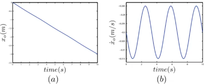
as shown in Fig. 7. The Fig. 8(a-b) plot the axial position and

x

y

Fig. 7. Worm locomotion in xy plane

velocity of the worm’s head with respect to time, respectively.

0 1 2 3 4 5 6 7 8 9 10 −3.5 −3 −2.5 −2 −1.5 −1 −0.5 0 time(s) xo (m ) (a) 0 2 4 6 8 10 −0.315 −0.31 −0.305 −0.3 −0.295 −0.29 −0.285 time(s) ˙xo (m/ s) (b) Fig. 8. (a) Time vs head position; (b) Time vs head velocity

The inverse locomotion dynamics and the inverse internal dynamics of the system are solved to get the reaction forces

at the anchorage points and the internal control forces,

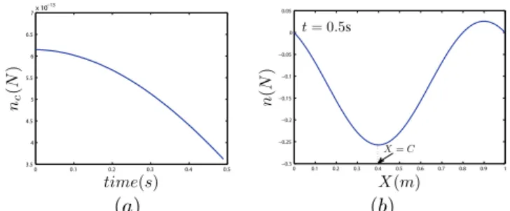
re-spectively. By taking the speed c = 0.3m/s as constant, it

is noted that the axial contact force is zero at the anchorage

point as shown in Fig. 9(b) at X = C where no force jump

renders the internal force profile discontinuous. This scenario may be compared to that of a wheeled body with constant velocity where the wheels (and hence the body) experiences no external (axial) forces so undergoing a pure inertial mo-tion. Furthermore, by introducing the time dependent speed

0 0.1 0.2 0.3 0.4 0.5 3.5 4 4.5 5 5.5 6 6.5 7 x 10−13 time(s) nc (N ) (a) 0 0.1 0.2 0.3 0.4 0.5 0.6 0.7 0.8 0.9 1 −0.3 −0.25 −0.2 −0.15 −0.1 −0.05 0 0.05 X(m) n (N ) t = 0.5s X = C (b)

Fig. 9. With constant speed: (a) Contact force; (b) Internal force distribution over the length

c(t) = at + b (with a )= 0), it is noted that, due to the worm

accelerations, the axial reaction force (nc) at X = C is not

zero anymore as shown in Fig. 10(a), and hence introduces a

jump on the internal control force at X = C. This appears

on Fig. 10(b) which gives the desired internal control force profile applied between cross sections over the whole length.

0 0.1 0.2 0.3 0.4 0.5 −10.5 −10 −9.5 −9 −8.5 −8 time(s) nc (N ) (a) 0 0.1 0.2 0.3 0.4 0.5 0.6 0.7 0.8 0.9 1 −6 −5 −4 −3 −2 −1 0 1 2 3 X(m) n (N ) t = 0.5s X = C (b)

Fig. 10. With variable speed: (a) Contact force; (b) Internal force distribution over the length

B. Caterpillar (Inchworm) in 2D

We now consider the case of a climbing robot bio-inspired from inchworms. Such an animal can be modeled as a bending

actuated beam with one localized clamping in C alternating

from one end to the other at each "step". Such a continuum robot can be modeled by a Kirchhoff planar beam actuated in curvature, i.e. by invoking the previous general construction

withG = SE(2) and ξd(t) = (1, 0, KdZ)T which in this case

(planar configuration) is an integrable variable as KdZ = θ%

where θ is the angle that parameterizes the absolute orientation of the cross sections in the plane. Having said that, the loco-motion of the caterpillar can be modeled by considering it as a continuous manipulator whose "base" and "terminal" change places at each half-period of its gait. In these conditions, the

previous algorithm (with the anchorage point fixed inX = 0)

can be run again by changing X into l − X in the spatial

ODE and at each half-period such that C = l. The gait can

be simply defined by the angle θ as:

θ(X, t) = α sin2(ωt) sin ! 2π l (X − l) " , (46)

from which the curvature law is derived:

KdZ(X, t) = α sin2(ωt) ! 2π l " cos ! 2π l (X − l) " . (47)

This law ensures that, at each instant: θ(t, X = 0) = θ(t, X = l) = θ(t, X = l/2) = 0 whereas the curvature is minimal

at the two ends and maximal at X = l/2. Finally, the time

function as a factor of this internal shape law ensures the periodic relaxation and bending of the robot. Its period is π/ω and it assures the amplification of the bending over a

half-period and its attenuation (down to 0) in the following

half-period. Thus, assuming that the caterpillar starts att = 0

in a stretched position, there will be anchorage atX = 0 at

all the intervals [2kT, 2kT + T /2] and anchorage at X = l

at the intervals [2kT + T /2, (2k + 1)T ]. In these two cases,

the external movements are null as they are fixed by the

anchorage conditions: X1(C) = (1, 0, 0). Moreover, the

external dynamics enable the reaction at the anchorage point to be calculated. Finally the internal dynamics can be easily

integrated (in this case ζ= ˙η) to give the internal wrenches.

x

y −→g

Fig. 11. Caterpillar locomotion in xz plane

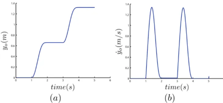
Numerical application: Some numerical results are obtained for caterpillar climbing under gravity by applying the curvature (shape)

law (47) as input, with α = 1.8

and ω = 2π0.25. Simulating for

14 sec, we get the motion of

the caterpillar in the xy plane

as shown in Fig. 11. The Fig. 12(a-b) plot the axial position and velocity of the caterpillar’s head with respect to time, respectively. The inverse locomotion dynamics and the inverse internal dynamics of the system are solved to get the reaction forces at the anchor-age points and the internal con-trol torques, respectively. The Fig. 13(a) shows the reaction torque

cz(X = 0) at head with respect

to time. For illustrative purpose, the torque distribution along the length is presented in Fig. 13(b)

att = 4.5s.

C. 2D snake in lateral undulation

A snake in lateral undulation is modeled by either a

Kirch-hoff or a Reissner 2D beam whose discrete counterparts are

drawn in Fig. 14(a-b), respectively (the beam cross sections being the continuous infinitesimal counterparts of the axles of the discrete mechanisms). In a first time, we choose the

0 1 2 3 4 5 6 0 0.2 0.4 0.6 0.8 1 1.2 1.4 time(s) yo (m ) (a) 0 1 2 3 4 5 6 0 0.2 0.4 0.6 0.8 1 1.2 1.4 time(s) ˙yo (m/ s) (b) Fig. 12. (a) Time vs head position; (b) Time vs head velocity

0 1 2 3 4 5 6 0 0.5 1 1.5 2 2.5 3 time(s) cz (Nm ) (a) 0 0.1 0.2 0.3 0.4 0.5 0.6 0.7 0.8 0.9 1 −2.5 −2 −1.5 −1 −0.5 0 0.5 X(m) t = 4.5s τ (Nm ) (b)

Fig. 13. (a) Reaction torque at head; (b) Internal torque distribution over the length

Kirchhoff-snake kinematic model because it is the simplest and it corresponds to the ACM robots of Hirose [1] whereas the second, as proposed by Ostrowski [36], although more complex, has advantages that we will mention later. In lateral undulation, the snake supports itself laterally in its environ-ment to self propel in an axial direction, i.e. by moving along the length of its backbone. Mathematically, these supports are modeled by non-holonomic constraints preventing the cross sections of the snake to slide laterally. In the case where the contact with the ground is continuously distributed along the body length, there are obviously enough of these constraints for the external movements to be completely fixed by the internal kinematics of the snake according to the kinematic context of section VII. In order to establish this kinematic model, we begin by writing the continuous model of velocities

(7) in the case ofG = SE(2) and ξd(t) = (1, 0, KdZ)T. Thus,

with η= (g−1_˙g)∨_{= (V} X, VY, ΩZ)T, we have:   V % X V% Y Ω% Z   =   VYKdZ ΩZ− VXKdZ ˙ KdZ   . (48)

By modeling the contact at each point X by a CSFS model

(section VI-B), the constraints are simply writtenVY(X) = 0,

for∀X ∈ [0, l] (the obstacles being fixed to space). Now, by

forcing these (non-sliding) constraints in (48), one obtains the relations which must verify every motion compatible with the

supports: _  V % X ΩZ Ω% Z   =   0 VXKdZ ˙ KdZ   . (49)

From the first line of (49), we see that the axial speed of

the snake is constant relative to X and thus equal to that

(a) (b)

Fig. 14. (a) Kirchhoff-snake; (b) Reissner-snake

of its head, which we will denote more simply Vo (every

function evaluated in X = 0 is indicated with a subscript

zero). From the second line, we see thatΩZ = VoKdZ, i.e. the

angular velocity along the snake’s backbone is only governed

by the forward speed Vo and the body curvature KdZ. Next,

taking account of lines 1 and 2 in the third, one obtains the fundamental relation:

˙

KdZ = VoKdZ% , (50)

which must be verified all along the snake so that its mobility (axial propulsion) is assured. Finally, the solutions of (50) take the general form:

KdZ(X, t) = f (X +

$ t

0

Vo(τ )dτ ), (51)

which corresponds to the propagation of a given curvature profile along the backbone at a generally time-variable speed

Vo(t) (see Fig. 15). It follows that such a choice of the

0 !1.5 !1 !0.5 0 0.5 1 1.5 2 2.5 3 X Kdz Vo Vo Vo l

Future Present Past

Fig. 15. Curvature profile along the snake’s backbone

curvature law ensures the thrust in the direction of−tX(0) at

the space-constant speed Vo(t). Moreover, for all X ∈ [0, l],

one can write:

ηo= ! Vo Ωo " = ! 1/K% dZ KdZ/K_dZ% " (X) ˙KdZ(X, t), (52)

and, particularly, forX = 0:

ηo= ! Vo Ωo " = ! 1/K% o Ko/Ko% " ˙ Ko, (53)

which generalizes the connection of the discrete case which encodes the follower-leader kinematics of snakes in lateral undulation. It is worth noting that, just as in the discrete case where the first three axles (starting from the head) fix com-pletely the motion of the head and that of the following links; in the continuous case, the connection (53) involves at most

the third derivative of the position field (i.e.K%

dZ(0) = r

%%%

(0)). In the continuous setting, the principle of the follower-leader kinematics can be stated as follows: once the curvature and its

derivative in∀X are specified, the velocity of curvature must

the cross section X at the speed Vo(t). Thus, every cross

sectionX reoccupies at t∗

such that+_tt∗Vodτ = X, the same

configuration as that occupied by the head at t. This explains

the impression of lateral stasis and axial movement observed in snakes, which makes their motion resemble a fluid line of a steady flow. In addition, (53) shows that if the axial propulsion

is assured by ˙Ko/Ko% it isKothat steers the snake in the plane.

Thus, we can approach the2D snake by analogy with another

non-holonomic system, more familiar to the robotics engineer: the car-like platform. In this case, the angular steering of

the (virtual) front wheels is ensured by Ko while the thrust

produced by the engine is assured by the relation ˙Ko/Ko%.

Turning back to biology, in nature, the curvature along the body of a snake changes according to the choices made by its head, choices that depend on the obstacles that the snake avoid and on which it laterally pushes to propel itself forwards. Consequently such a situation may be represented by a steady

profile of curvature moving at the speedVo(t) along the body,

represented here by the material segment [0, l] (see Fig. 15

where such a context is illustrated). Finally, for illustration

purpose, let us consider the case where ˙Vo= 0, then (50) turns

to be the one-dimensional propagation equation whose general

solutions areKdZ(X, t) = f (t + X/Vo), with Vothe constant

speed of the curvature waves. Then, for environments without obstacles but where the ground plane has good properties to prevent lateral sliding, the law of curvature:

KdZ(X, t) = a cos(ω(t + X/Vo)) (54) + b exp ! − (t − (to+ To/2) + (X/Vo)) 2 (t − (to+ To/2) + (X/Vo))2− (To/2)2 " ,

ensures, up to t = to, an axial speed −VotX(0) of average

constant direction, and from t = to generates a turning

maneuver of duration To. Next, note that these kinematics

are singular when KdZ = cte/X because, in this case, the

conditions of mobility (50) are not verified except in the irrelevant case where the snake has a null motion. To overcome this situation, one can consider the continuous homologue of the discrete kinematics of the Fig. 14(b), i.e. by adding a transverse shearing to the present context. In this case, the kinematics become those of an actuated Reissner planar beam and the continuous model of velocities is rewritten from (48), replacing the first line by the following:

VX% = −KdZVXΓdY, (55)

so that we now haveVX(X) = Vo e(

−!X

0 KdZΓd YdX) and the

mobility condition (50) becomes the following: ˙

KdZ = (KdZ% − KdZ2 ΓdY)VX, (56)

where the presence of the control parameter ΓdY as a factor

of KdZ ensures the mobility of the snake in all cases where

KdZ(.) )= 0. Thus, we recover that the continuous homologue

of the discrete kinematics of the Fig. 14(b) is only singular for the straight configurations as it is only in this case that the internal movements of the odd and even joints cannot produce external movement. Finally, in the case of snakes, the transverse shearing models the movements of the skin and the scales relative to the skeleton whose own movement

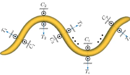
C1 C2 C 3 Ci Cp Ti T1 T2 T 3 Tp

Fig. 16. 2D snake with p contacts

is modeled by the field of curvature. Also, if a snake finds itself in a perfectly straight configuration, it can remove itself

from this singularity by: 1) sliding laterally, 2) leaving the

ground. However, if these two possibilities are forbidden (for example, if the snake is made to pass through a straight narrow tube), then only a mode of locomotion like that studied for the earthworm in traction-compression becomes possible.

Finally, as for the net motions computation, taking account of (53), the locomotion kinematics (34) of block0 (Fig. 5) can

be written as the system in SE(2):

˙go= goηˆo= go   1/K % o 0 Ko/Ko%   ∧ ˙ Ko. (57)

For the forces, the algorithm integrates at each time-step t,

the system (25) from X = 0 to X = l initialized in space

by (go(t), ηo(t), 0, 0, 0). Then, knowing ˙ηo(t) from the time

derivative of (53), the algorithm computes in block1 (Fig. 5) via (35) the resultant of the contact wrenches reduced to the

head i.e. Fc. Knowing this resultant, we must formulate a

hypothesis for the distribution of the contact forces in order to compute the distribution of the internal forces and torques. For example, assuming that the snake is permanently in contact

with the ground via p supports whose positions are fixed in

space as indicated on Fig. 16. Then the load is generally

hyper-static (whenp > 3), and the determination of the lateral

contact forces distribution:Ti=1,2,..p, requires the generalized

inversion of the under-determined system:

Fc = i=p * i=1 Ad∗ k(Ci)   T0i 0   , (58)

where we recall thatk(Ci) = g−1(Ci)go(t), and we consider

the motion while thep points of contact C1,2,..p are contained

in ]0, l[ (see Fig. 16). Once these p forces are known, the

algorithm can integrate in block2 (Fig. 5) the internal dynamics

(23) with initial spatial conditions:(go(t), ηo(t), ˙ηo(t), 0) and

a distribution of external forces4_{:F =})p

i=1(0, Ti, 0)Tδ(X −

Ci).

Numerical results:In case of the 2D snake, an undulatory gait of the type (54) is imposed as input of the algorithm

(of section VII). The undulation is provided with b )= 0 for

4_{This can be achieved by piece-wise integrating the internal dynamics on} [0, C1] ∪ [C1, C2] ∪ ...[Cp, l], using the jump conditions: N (Ci−) = −Ti+ N(Ci+) and M (Ci−) = M (Ci+) where (NT(Ci−), MT(Ci−))T and (NT_(C

i+), MT(Ci+))Trespectively denote the material wrench of internal forcesΛ evaluated on the left and the right sides of the cross section Ci.

certain period of time To which quantifies the amplitude of a

turning maneuver inSE(2), where a = 10, ω = 2πVo/λ and

Vo = −0.5m/s. Simulating for 10s, the 2D motion of the

snake in the xy plane is shown in Fig. 17. Furthermore, the

x

y

Fig. 17. Snake turning locomotion

locomotion and internal dynamics of the system are solved for p = 5 to obtain the cross sectional reaction wrenches applied

at the contact pointsC1, C2, ...C5(see Fig 16) and the internal

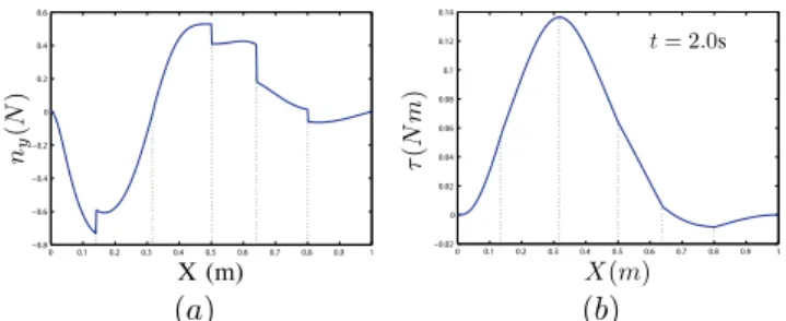
control torques, respectively. The Fig. 18(a) plots the reaction

force (ny) over the length. The Fig. 18(b) shows the torque

distribution over the length of snake at t = 2.0s.

0 0.1 0.2 0.3 0.4 0.5 0.6 0.7 0.8 0.9 1 −0.8 −0.6 −0.4 −0.2 0 0.2 0.4 0.6 X (m) ny (N ) (a) 0 0.1 0.2 0.3 0.4 0.5 0.6 0.7 0.8 0.9 1 −0.02 0 0.02 0.04 0.06 0.08 0.1 0.12 0.14 X(m) t = 2.0s τ (Nm ) (b)

Fig. 18. (a) Contact force (ny) over the length; (b) Internal torque distribution over the length

D. 3D snake in lateral undulation

Here we consider only the kinematic aspects of 3D

crawl-ing. The 3D snake is a priori modeled by Kirchhoff

kine-matics with torsion. In this case, we have G = SE(3) and

ξd= (1, 0, 0, KdX, KdY, KdZ)T so that the kinematic model

(7) is now written:         V% X V% Y V% Z Ω% X Ω% Y Ω% Z         =         VYKdZ− KdYVZ ΩZ+ KdXVZ− VXKdZ −ΩY + KdYVX− KdXVY ˙ KdX+ ΩYKdZ− ΩZKdY ˙ KdY + ΩZKdX− ΩXKdZ ˙ KdZ+ ΩXKdY − ΩYKdX         . (59)

On the basis of this model, we shall first research the3D

ho-mologue of the gaits previously exhibited in2D. This requires

establishing the constraints of non-sliding in 3D, which is simply achieved by proposing that, for every material abscissa

X, the contact is modeled by a cross sectional follower support

so that using (32) withΩcX = VcY = VcZ= 0, one has:

VY(X) = VZ(X) = 0 , ΩX(X) = 0, ∀X ∈ [0, l], (60)

which are 3 non-holonomic constraints that must verify each of the cross sections in movement. Next, we introduce these relations into the general kinematic model (59). As a straight-forward consequence, the first three equations of (59) allows one to write:

VX = Vo ,ΩY = VoKdY ,ΩZ = VoKdZ, (61)

whereVo is again the axial uniform speed along the backbone

while the two last of these relations translate the fact that the internal angular velocity of the cross sections is entirely due to the axial movement along a given profile of fixed curvature. Now taking into account the above relations in the fourth

equation of (59) in whichΩX= 0 is forced, we simply find:

˙

KdX = Ω%X+ ΩZKdY − ΩYKdZ

= 0 + Vo(KdYKdZ− KdZKdY) = 0. (62)

Thus, if we assume that the robot starts (at t = 0) from a

straight untwisted configuration, one haveKdX = 0 all along

its length and at any instant of the motion. Introducing this last constraint as well as all the others into the two last relations of (59) allows one to write with (62), the three independent relations on the strain laws:

  ˙ KdX ˙ KdY ˙ KdZ   =   0 K% dYVo K% dZVo   , (63)

where the first of these relations can be ensured by the design (un-twistable kinematics) while the two others are imposed by the curvature control laws. Finally (63) defines the 3D counterpart of the planar mobility condition (50). Continuing

in the same way as for the2D case, we find the 3D external

kinematic model in the form of the follower-leader connection:

˙go= go     Vo 03×1 ΩoY ΩoZ     ∧ = go     1/K% o 03×1 KoY/Ko% KoZ/Ko%     ∧ ˙ Ko, (64) with ˙Ko= *Kd*!(0) et K% o= *Kd*%(0).

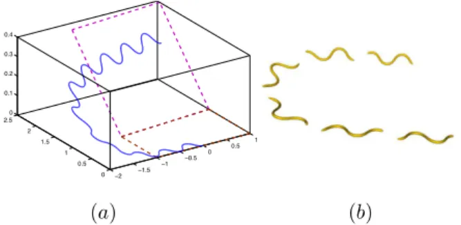
Numerical results: In case of 3D snake, the undulatory motion (54) along with:

KdX(X, t) = 0, KdY(X, t) = by exp ! − (t − (to+ To/2) + (X/Vo)) 2 (t − (to+ To/2) + (X/Vo))2− (To/2)2 " ,

is given as input to the general algorithm, with a = 10, ω =

2πVo/λ, by = 0.5 and V o = −0.5m/s. Simulating for 10s,

the 3D motion of the snake in the xyz space is obtained as

!2 !1.5 !1 !0.5 0 0.5 1 0 0.5 1 1.5 2 2.5 0 0.1 0.2 0.3 0.4 (a) (b)

Fig. 19. (a) Head turning locomotion; (b) Snapshots of snake3D turning locomotion

IX. GENERALDISCUSSION ANDCONCLUSION

In this article, we have proposed a general abstract frame-work for modeling continuous style like robots at a macro-scopic scale. The solution turns out to be a continuous coun-terpart of the Newton-Euler dynamics of discrete multibody systems, where the robot is here considered as a strain-actuated Cosserat beam i.e. a serial continuous multi-body system. Once embedded in the framework of locomotion theory on fiber bundles, the approach is exploited to derive an algorithm capable of computing the torques as well as the rigid net motions involved in any locomotion task. The approach as a whole is applied to the case of on ground locomotion where the model of external forces is replaced by the kinematic holonomic and/or nonholonomic constraints of a set of models of contact of practical interest in terrestrial locomotion. It is then applied to several examples inspired by natures. Through these examples, it shows that it can be a useful tool of investigation when it is applied to the analysis of mobility or gait generations of snakes. In the case of earth-worm, the Cosserat assumption of beam cross sections rigidity is removed and replaced by the axial volume preservation constraint. This allows with small efforts to extend the approach and the algorithm to one dimensional hydrostats. The problem of manipulation is illustrated indirectly through the example of the climbing inchworm where at each step of the "walking" the robot is a manipulator clamped into the ground.

Finally, in a second step the question of how applying these results to real designs naturally arises. About this point, the proposed approach being general, the cost to pay for this generality is a certain idealization of the model. This

idealization essentially concerns two points: 1◦) the model

of the body as an internally actuated Cosserat beam. 2◦

) the model of the contacts between the body and its surroundings. As regards the first point, we today suggest to proceed case by case. For instance, for a specific technology among the numerous designs of snake-like robots today developed [37], [38], one could first ask the starting questions: does the basic Cosserat assumption of rigid cross sections have a physical reality? And also, how this assumption can be adapted to a particular technological principle? As a first answer, let us remark that in the case of designs inspired from vertebrate animals where one can identify lateral rigid elements attached to a body line axially articulated and mimicking the backbone, the Cosserat model is more and more well adapted as the number of vertebrae increases (big snakes like pythons can have more than several hundred). In a design more inspired

from hyper-redundant arthropods, the rigid segments can also be considered as being the cross sections of their macro-continuous model. Finally, for robots inspired from hydrostats, although the application of the approach seems less natural since these animals do not contain any rigid element in their principle, we saw in the article, how we could release the Cosserat basic assumption of rigid cross sections in order to adapt the model to a simplified version of one dimensional hydrostats. Furthermore, some groups today exploring new designs in soft robotics have chosen to mimic hydrostats as a set of rigid cross-sections interconnected and through actuated cables and refer explicitly to the Cosserat model as a source of inspiration for their design [7]. Finally, as elasticity plays an important role in continuous robots, the body model proposed in the article could be improved in this sense. About the second point (the model of the contacts), let us remind that in the case of snake-like robots, we have modeled the contacts through bi-lateral annular joints introducing a null axial friction (along the vertebral axis) as well as an infinite lateral friction force (perpendicular to the vertebral axis). In spite of its ideal character, such a model is not so far from what one can observe on real snakes. Indeed, the scales of the snakes give to their skin a strong frictional anisotropy, the axial friction being far lower than its lateral counterpart. In our case, we pushed this tendency to its ideal asymptotic limit, and also replaced the usual unilateral contacts by bi-lateral constraints. This second simplification, which can be released in future, requires a further discussion on the feasibility of a motion. Indeed, once the net motions known by solving the external kinematics, one has to check whether the real contacts can generate the desired external wrench? Technically, the answer to this question depends on the solutions of a linear

system of the form5 _{(58). In particular, if the joints are in}

reality unilateral contacts (as this is the case of obstacle-aided locomotion [37]), the reaction forces solutions of (58) should have to keep a given sign all along the motion. At last, once such a loading has been found, so validating the model of contacts, one has to check whether the actuators can supply the desired motions under such a loading. In order to address this last problem, one can use the inverse dynamics of control torques. Now, coming back to nature, for a snake moving in a tree for instance, the animal permanently exploits the redundancy of (58) in order to satisfy supplementary more sophisticated conditions as maximizing the adherence while minimizing the consumed energy... Among the degrees of freedom of these solutions that the snakes exploit, they can change the configuration of the contacts with time and play with the internal control forces which do not produce any net motion. Finally, if we seek a design of snake-like robot ideally adapted to our model of robot and contacts, starting from [39], this would be a multi-body system with a very high number of very small length links connected through universal joints. Each of these links would be equipped with many wheels aligned along its greater length and placed radially on the links, so bio-mimicking the scales of a 3D snake (see Fig. 20). Finally, as the number of the links increases, it becomes