.t ... LfU..,rAr 28-S2."0::,
. , ..
E. MASAC..HUSES INSTITUTE OF TECHNOLOGY
CA~lBlljGE 89, MASSACMUS2TTS, U.S.A&
L
A 6/
Y
3
AN ANALYSIS AND SYNTHESIS PROCEDURE
FOR FEEDBACK FM SYSTEMS
ANDRZEJ WOJNAR
TECHNICAL REPORT 415
SEPTEMBER 30, 1963
MASSACHUSETTS INSTITUTE OF TECHNOLOGY RESEARCH LABORATORY OF ELECTRONICS
CAMBRIDGE, MASSACHUSETTS
,
The Research Laboratory of Electronics is an interdepartmental laboratory in which faculty members and graduate students from numerous academic departments conduct research.
The research reported in this document was made possible in part by support extended the Massachusetts Institute of Technology, Research Laboratory of Electronics, jointly by the U.S. Army (Signal Corps), the U.S. Navy (Office of Naval Research), and the U.S. Air Force (Office of Scientific Research) under Contract DA36-039-sc-78108, Department of the Army Task 3-99-25-001-08; and in part by Signal Corps Grant DA-SIG-36-039-61-G14.
Reproduction in whole or in part is permitted for any purpose of the United States Government.
MASSACHUSETTS INSTITUTE OF TECHNOLOGY RESEARCH LABORATORY OF ELECTRONICS
Technical Report 415 September 30, 1963
AN ANALYSIS AND SYNTHESIS PROCEDURE FOR FEEDBACK FM SYSTEMS
Part A: Conventional FM Systems Part B: Feedback FM Systems
Andrzej Wojnar
(Manuscript received February 27, 1963)
Abstract
An investigation of frequency-compressive feedback FM systems has been made, with emphasis placed on threshold behavior.
In Part A, following a survey of the existing noise analysis of FM systems, use is made of a recent evaluation of the impulsive noise component which is due to Rice. It is shown that this excess-noise component predominates in the threshold region of most conventional FM systems. A new analytical expression (which agrees with experimental evidence) has been found for the location of the noise threshold.
In Part B, two possible mechanisms causing noise threshold in a feedback FM sys-tem are examined. It is shown that the feedback threshold results in an abrupt break-down of system performance, and therefore should not be approached too closely. It is therefore recommended that feedback systems be designed with the conventional threshold predominant. In this case, the analysis of feedback systems approaches that of conventional systems. Some modified formulas for feedback FM system performance at threshold are proposed; new bounds on the performance of the systems with optimum feedback filters are derived. The maximum obtainable threshold power-bandwidth trade-off implied thereby is also determined. Experimental results with certain feedback FM configurations are reported. The experimental investigation verifies some synthesis rules and certain of the analytical results, but some aspects of the system threshold behavior still require further investigation.
TABLE OF CONTENTS
PART A: CONVENTIONAL FM SYSTEMS
1. Noise Performance 1
2. Simplified Analysis of the Strong-Carrier Case 3
3. Simple Approach to the Threshold Problem 6
4. Analysis of the Impulsive Noise 8
5. Evaluation of Threshold 11
6. Performance Analysis of Conventional FM Systems 14
PART B: FEEDBACK FM SYSTEMS
7. The Concept of Frequency-Compressive Feedback 19
8. Noise Threshold in the Feedback System 20
9. Analysis of the Feedback Threshold 22
10. Analysis and Catalog of Feedback Filters 25
11. Synthesis of the Feedback System 28
12. Optimization of the Feedback FM System 33
13. Experimental Program and Apparatus 36
14. Summary of Experimental Results 40
Acknowledgment 47
PART A: CONVENTIONAL FM SYSTEMS 1. Noise Performance
Ultimate limitations in the performance of communication systems are imposed by random noise at the receiving end. In the first part of this report we shall present an analysis of conventional FM systems disturbed by additive fluctuation noise. In the
sec-ond part, we consider the frequency-compressive feedback case.
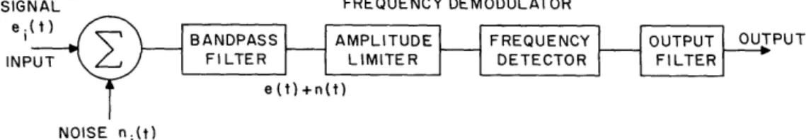
In order to analyze an FM system, we shall use an idealized mathematical model. The model (Fig. 1) consists of a symmetrical narrow-bandpass filter, an ideal broad-band limiter with zonal filter, and an ideal frequency detector that operates in quasi-stationary fashion and is followed by a lowpass filter.
Under certain plausible assumptions2 the input noise can be considered to be derived from a white Gaussian noise source, and the input to our frequency demodulator to be the sum of an FM signal and narrow-band Gaussian noise. The analysis is then reduced to differentiation in time of the phase angle of the composite wave.
After the detector output wave has been expressed as an implicit time function, the Fourier transform of its correlation function yields the spectrum of the demodulated noise. A straightforward filtering operation then gives the output spectrum and the total output noise power.
A great deal of information has resulted from analyses of this sort by Rice,3 Stumpers,4 and Wang5 with regard to the rectangular and normal-law bandpass filter cases. Extended analysis by Middleton6 - 8 has also covered more general cases of nonideal amplitude limiting and several different filter structures.
The nonlinear interaction between signal message and noise has been carefully inves-tigated, in this same way, but leads to prohibitively complicated mathematical expres-sions. Some important cases have been evaluated by numerical computation and shown in graphs of input-output relations.4'7'8 The analysis of limiting cases has always been quite well advanced; thus a general picture of the whole area emerges as a composite of several different regions, each characterized by different components of output noise. For this reason, different definitions of the noise threshold are also possible. 2'9
Early attempts to translate the analysis into system-oriented signal-to-noise ratio formulas and charts7 ' 1 0 were adequate to meet some needs of conventional FM
SIGNAL FREQUENCY DEMODULATOR
e.i INP
NOISE n (t)
Fig. 1. Model of the FM receiving system.
1
engineering until the advent of feedback FM systems. New problems are now arising from new system principles and, thanks to phenomenological investigations, more insight into the physical character of output noise has been gained. Therefore a strong trend toward modifying the conventional (correlation function) analytic approach - which is more suitable for linear-modulation systems - parallels the research on hitherto unex-plored (or unsatisfactorily exunex-plored) areas. As a result, important new contributions that are concerned with the structure of the nonlinearly processed noise are beginning to appear.
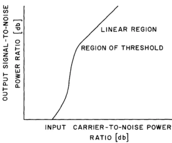
In this report, we shall first survey and explore certain new results of an analysis which facilitate the resolution of output noise into different components. Looking upon the input-output relations in an additively disturbed FM system, we propose consider-ation of the following regions of interest (Fig. 2):
(a) Strong carrier, weak noise: The output noise is nearly Gaussian, and linear superposition with message holds. This is the only region of unrestricted practical usefulness.
(b) Region of noise threshold: Two sharply rising components (quasi-Gaussian and impulsive) of output noise are superimposed on the output signal. Practical interest is confined to the boundary between regions 1 and 2.
Below the threshold, superposition does not hold any more; a pronounced fall in out-put signal power occurs until the message is fully captured by the disturbance. The well-defined limiting case of noise alone (no carrier) is sometimes used as a reference point (cf. the noise-quieting sensitivity).
For the model considered above, the input carrier-to-noise power ratio (CNR) is the only major parameter influencing the system performance. Conventionally, the latter has been expressed in terms of the output signal-to-noise power ratio (SNR). But it does not seem meaningful to cover both regions of interest with this single measure
of performance. w () 0 z _J z (. 09 o, I-0
INPUT CARRIER-TO-NOISE POWER RATIO [db]
Fig. 2. Input-output relation in an FM system.
2
Additional hazard is also involved in plotting the signal-to-noise ratio over a wide range of variables, when the available numerical results are, in fact, limited to small
ranges of values. For example, exploiting the analysis and computations by Rice,3 Skinner in an unpublished memorandum10 aimed at graphical presentation of the system performance over a wide range of CNR. Unfortunately, his plot was obtained by fairing together the different available graphs for fragments of the individual regions. In the
important region of threshold, the necessary accuracy was missing. As a result, the threshold curve derived therefrom by Replogle 1 is far from accurate and can be
mis-leading, as we shall see in Fig. 5.
This report will, in general, be confined to the analysis of regions 1 and 2 described above, both of which are characterized by the absence of first-order interaction between noise and signal. After recapitulation of known data, some extension of the existing noise analysis will be presented. The effective disturbance in these regions can be attributed to an additive noise rather than involving nonlinear distortion of the message also.
2. Simplified Analysis of the Strong-Carrier Case
Consider our idealized FM system in Fig. 1 to be disturbed by white Gaussian noise with spectral power density equal to N so that, after bandpass filtering, narrow-band Gaussian noise of the form
n(t) = nc(t) cos wct - ns(t) sin Oct (1)
enters the frequency demodulator. The FM signal at the same point may be expressed as
e(t) =Q cos [ct + (t)] (2)
where the carrier amplitude Q and the carrier frequency oc = 2Zfc are constants. The message is bandlimited and is contained in the time derivative of the signal phase
angle, ' (t).
Assuming that the filtered noise is weak relative to the carrier, and denoting the demodulator input sum as
e(t) + n(t) = V(t) cos [ct + (t) + e(t)], (3)
we are interested first in determining the additive disturbance 0'(t) at the output of the demodulator. Assume that part of the output filter suffices to pass all the message, but
sharply cuts off the higher frequency components of 8'(t), in order to improve the out-put SNR. We shall evaluate the effect of this filtering in terms of output noise spectrum
and power.
Let us further denote the (positive frequency) power density spectrum of the I-F noise by w(f) which (within a multiplicative constant) equals the squared magnitude response of the bandpass filter. With the demodulator input average CNR denoted by r,
3
we have the obvious relation
Q2/2 Q2
r = _ - (4)
z(t)
z
JO w(f) dfn t)
which holds with arbitrary modulation (and also for O = 0).
We first state that region 1 is characterized by r >> 1 so that the noise magnitude
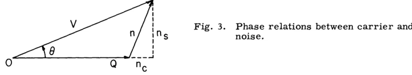
Fig. 3. Phase relations between carrier and
inS noise.
In(t) is nearly always much smaller than Q. In the simplest case of an unmodulated carrier, the input signal and noise combine as visualized in Fig. 3, and we easily find that
-1 n(t) ns(t)
e(t) = tan Q (5)
Q + n (t)
Rigorously, this approximation holds true within an additive multiple of 2r.
When the filter response is symmetrical about fc, the power density spectrum of nc(t) and ns(t) has been found3 to be Zw(fc+f). Therefore the normalized* power den-sity spectrum of the derivative ns(t) equals f . 2w(fc+f), and the power denden-sity spec-trum, W(f), of the disturbance '(t) ns(t)/Q can be expressed approximately as
W(f) f2 X 2w(fc+ f)/Q 2 , (6)
provided that r >> 1.
The above-mentioned treatment of FM noise was initiated by Crosby,l2 who con-sidered the simplest case of rectangular filters and white noise. Denoting the input (intermediate-frequency) filter passband by B and the output lowpass band by fa, we may repeat Crosby's integration in order to find the output power N of the (weak) Gaussian noise. We obtain
f f3
N = W(f) df =a (7)
3rB
Here normalization consists in assuming that the demodulation constant and the load
4 resistance are unity and dimensionless.
-BANDPASS FREQUENCY OUTPUT
FILTER DETECTOR FILTER
CARRIER Q OUTPUT
IINPUT "
NOI o S E/ |' NOISE
UNITY SLOPE
LOWPASS FILTER DIFFERENTIATOR OUTPUTFILTER
INPUT OUTPUT
NOISE 2No/r NOISE
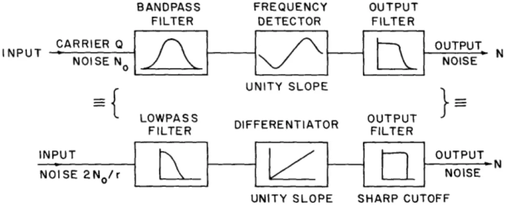
UNITY SLOPE SHARP CUTOFF Fig. 4. Linear model for noise transmission.
in normalized units.
It is clear that the noise output (7) from an FM system in region 1 is identical to that produced at the output of the three linear filters shown in Fig. 4, in which the demodulator has been replaced by a differentiator weighting the original spectrum by (f-fc)2. Thus, as far as noise analysis (with large CNR) is concerned, we can replace the actual nonlinear receiver of Fig. 3 by the linear model of Fig. 4, operating upon a white spectrum of input noise.
Although a rectangular bandpass filter may be regarded as a rough approximation for a chain of double-tuned intermediate-frequency filters (used in most conventional systems), it is not the only good noise-filtering arrangement. Let us define the equiv-alent noise bandwidth B of the input filter as
B
0
w(f) df, (8)w(fc )
and consider a family of different symmetrical narrowband input filters characterized by varying w(f) under the constraint that B remains fixed. It is conjectured from FM distortion theoryl3 that over a broad class of reasonable variations, the message trans-mission does not undergo significant changes. On the other hand, it is easy to see that a slow roll-off filter spreads the energy of FM noise outside of the output band, and thus contributes to the decrease of output noise power.
One convenient measure of the noise-power transfer through the first two units of the filter chain in Fig. 4 can be conceived2 in terms of p, the radius of gyration about the symmetry axis, defined by
2 I (f-fc) w(f) df
p =
(9)
fo
w(f) dfHere, the denominator describes the noise entering the demodulator, and the numerator
5
-the noise output from -the demodulator.
In the complete filter chain of Fig. 4, the effect of the sharp-cutoff output filter is to chop off the output spectrum at fa' This, however, can also be accounted for by imposing a finite limit of integration in the numerator of Eq. 9. We therefore define for the baseband analog another coefficient Pa, describing the noise transfer in the entire chain: f 2 foa 2f2w(fc+f) df D= . (10) a 0 w(f)df 0
All of these definitions apply to the output of any symmetrical bandpass filter. They have been introduced primarily because the output noise power of the system can then be expressed by means of the simple relation
N = p2/2r, (11)
which follows directly from (7), with appropriate substitution of (4), (6), and (10). Notice 1
that for f >> a2 -B we have in the limit Pa a p; more important is the case of narrow-band lowpass filtering with fa << 2 B because, then, to a first-order approximation, the
noise output does not depend greatly on the shape of the bandpass spectrum w(f), pro-vided that the former is symmetrical and flat in the middle.
It will prove useful in the sequel to present in Table 1 a compilation of the properties of some filtering arrangements. The normal-law filter has been included as a good approximation to the cascade of many identical single-tuned filters; the single-tuned filter was evaluated because of its importance for the feedback FM systems. With our
1
interests limited to the region fa < 2 B, we have a well-defined Pa and the output power is bounded, even for the single-tuned filter. Also, the single-tuned filter really has good filtering capability in FM systems, as can be observed by comparing the values
of Pa' Or, still better, consider the ratio pa/B, which is one figure of merit for the filtering of noise, provided that B is regarded as a measure of the bandwidth required
for tolerable transmission of the signal message. 3. Simple Approach to the Threshold Problem
The exact graphical representation of noise output power as a function of input CNR 3-8
(see, for instance, the work of several authors ) clearly exhibits a relatively sharp break region. The question arises whether we can sensibly describe the location of the break, called the threshold, in the linear input-output characteristic of the system by one discrete value of input CNR. This approach, although mathematically questionable, nevertheless has important advantages in the analysis and synthesis of systems, and therefore seems to be worth following.
We are therefore in search of a border line to the linear (weak-noise) region. Recall
that the approximated linear equation (5),
0(t) ns(t)/Q,
holds in region 1, provided that r >> 1. Actually, three simplifying steps (corresponding to various excess-noise components) have been made in the approximation:
tan 1 n(t) ns(t)/Q, if and only if n << Q ns << Q Q + nc(t)
The first approximation consists of neglecting the relatively small summand in the denominator; the second replaces the arc tangent function by its argument - without adding the multiple of 2r, which is the third approximation. The usual procedure would be to determine the most restrictive of these three approximations, and to find its region
of validity. All three simplifying approximations may be significant, and considering but one of them may be misleading.
Let us, for the moment, follow the classical approach, disregarding the multivalued-ness of the arc tangent function. In order to find a significant departure from linearity, we shall choose an expansion for which the right-hand side of (5) represents the leading term. Such a result may be derived in terms of the mean-square values from Rice's asymptotic expansion3 of the autocorrelation function of , given in 1948. This expan-sion is expressed in terms of the autocorrelation function of the noise waveform n(t) n(t+T); at the origin (T = 0), by virtue of (4), we have
n2 = n2 = n2 Q2/2r (12)
in terms of the average carrier-to-noise power ratio r.
Evaluating Rice's equation (his Eq. 7.3) at the origin, we have in our notation: (n2)2
82n 1 +n +8 +
or
The same result can be obtained from the expansion of the arc tangent function in a power The same result can be obtained from the expansion of the arc tangent function in a power series, whereby the argument itself is represented by an expansion (compare also Eq. 10 in a recent paper by Baghdady14). Note that if the input is Gaussian, the first term of
(13) represents Gaussian output noise. The first-order correction term is an important component of excess noise; it is not Gaussian, but we may call it quasi-Gaussian. Obvi-ously, this noise term (when significant) will cause the input-output relation to depart from linearity. Now a simple inequality can be used to define the border of the linear
7
region, or the threshold caused by the quasi-Gaussian excess noise, say
1 1
1 >> 2 or rT > -c, (14)
where c is an arbitrary constant parameter, and the subscript "T" marks the threshold as a point rather than a region. A reasonable value for c, whereby (14) is satisfied, is c = 0.1; then we obtain rT = 5.
In accordance with this choice of c, a carrier-to-noise power ratio of approximately 5 times, or 7 db, would be needed to pass the threshold. The reader may be skeptical that such a low value will suffice, but it must be borne in mind that (13) does not neces-sarily show all sources of excess output noise. When entering the threshold region from the linear region, we do, of course, encounter this first-order nonlinear term, derived from Gaussian noise; however, another noise term of quite different character will also appear, which we shall now discuss.
4. Analysis of the Impulsive Noise
A very important contribution by Rice1 5 has recently provided a different approach to the analysis of noise in FM systems. In order to justify the significant conclusions drawn from Rice's argument, let us briefly summarize his new results.
Even well above the threshold, it sometimes occurs that over a short interval of time the magnitude of the random-noise vector in Fig. 3 exceeds the length of the car-rier vector and, simultaneously, the noise phase angle (tan-1 [nc(t)/ns(t)]) passes through +1r. We can then expect that the sum of carrier and noise will encircle the origin, and that the phase angle will rapidly be increased by ±+2r. Thus an impulse is produced in the 0'(t) waveform with an area of approximately ±2rr radians per second. After low-pass filtering, broadened impulses of either polarity appear in the output and are heard as clicks in the audio band, or seen as lengthy spots on the screen of an FM television system. Noise of this sort is related to the multivalued nature of the arc tangent func-tion (which has been neglected in secfunc-tion 3).
Rice succeeded in determining the expected number of "clicks" per second in terms of the input carrier-to-noise power ratio and of the parameters of the input filter. Assuming a Poisson distribution of the arrival times of the pulses, Rice also computed the corresponding power spectral density and the output power in the output band.
Above the threshold region, the two excess output-noise components (quasi-Gaussian and impulsive) seem to be uncorrelated. This being the case, a comparison with earlier results obtained by autocorrelation analysis could be performed by addition of noise terms on the power basis. This reasoning has been checked by Rice with numerical computations extending slightly into the threshold region. It must, however, be borne in mind that the impulsive noise is very specific in character and spectral distribution.
On the other hand, it appears that Rice's evaluation of impulsive noise can be explored in another way, and leads to a new measure of noise threshold. The
fundamental formula1 6 of Rice
2 00r 2
v = p(1-erf4Tr) = p eY dy, (15)
where p is the radius of gyration defined by Eq. 9, gives the expected total number, v, of (upward and downward) clicks per second in the threshold region and above it, with unmodulated carrier. The gyration radius of the symmetrical bandpass filter is, in general, proportionally related to its noise bandwidth (Table 1) so that, for a given fil-ter, v/B depends only on the carrier-to-noise power ratio, r.
The random succession of upward and downward impulses has a spectrum that is substantially flat at lower frequencies, whereas the Gaussian output noise spectrum is proportional to the square of the baseband frequency. In order to stress this difference, Rice denoted the constant power spectral density of the impulsive noise by W(O), and by straightforward reasoning obtained the result
W(O) z 2v = 2p(1-erf4J). (16)
With sharp-cutoff frequency of the output filter denoted by fa' the output power of the impulsive noise is evidently
-r
Ni 2Pfa( l-erfrr ) 2pfa e (17)
with no modulation present. Note, by comparing (17) with (13), that the impulsive excess-noise component differs substantially from the quasi-Gaussian one, which changes with input CNR as 1/r2
In a further step, Rice computed the effect of modulation on the impulsive noise, and found a significant interaction between message and noise. The number of clicks increases considerably with the signal-frequency deviation. Rice made an approximate evaluation for the case of sinusoidal modulation, whereby the frequency is deviated over the entire band of a rectangular bandpass filter. Simplifying Rice's result (his Eq. 2.26), we find that a first approximation to the value of impulsive-noise output power is given by
Ni 2 e rBfa, (18)
provided that r >> 1. A small correction term, diminishing the quasi-Gaussian noise in the same case, is also given by Rice.15
We shall now consider the location of the threshold in terms of the parameters of the impulsive noise. It will be shown that even with the noise power as a measure of
For the mathematical model of the single-tuned circuit we have a singularity because the gyration radius increases without bounds; no method of overcoming this difficulty has been found (S. O. Rice, private communication, 1963).
N E 'n rlm ml i ! .111 1-tt N mat I
I
mlI-I
1. t · t I. I__ ,.
m 10n klv I-IC Im m ID IF M 1 [t -< _; 0 z of alm a o -50 s'Rm I ,x 2 :Sai
N.0 rt + IL X X 3°J-a g Z(d 1_< II t I U, E to o o 0 r to 0 k .1 D " ii --W.O_ 04 0 44 am In 10 _ __ _ _ __ _ _ I-L-IM cq I: + .disturbance, the impulsive component is very significant, and, in fact, determines the extent of the linear region.
5. Evaluation of Threshold
Rice's results facilitate the physical interpretation of the threshold as being caused by the exponentially increasing impulsive component of output noise. As the first-order quasi-Gaussian excess-noise component is generally proportional to 1/r2 , it will be pre-dominant with a very strong carrier. As r decreases into the threshold region, how-ever, we find that the impulsive contribution imposes a more severe limitation on the extent of the region of linearity. Also, its character is especially annoying with some types of messages.
Let us examine the simplest case of rectangular input filter and unmodulated carrier. We shall first determine that value of r for which the power of the impulsive noise is no longer negligible in comparison with the linear Gaussian noise (11).
The threshold inequality, approximated by setting
1-erfrz 1 e- r (19)
now is
2 1 -r P
2pfa I- e r<< (20)
For the rectangular filter, we find from Table 1 that f3
B 2 2 a (21)
P - a 3B' (21)
so that the condition of Eq. 20 becomes
er (B Z -2 >> f (T_) B B
~~~~~~~~~~~~~(22)
The inequality can be treated similarly to (14), and this yields
r 2
c er . a) (23)
With c = 0.1, as before, we obtain a transcendental equation determining the threshold CNR:
2rT
e j/rT f B (24)
a
with the rectangular bandpass filter.
Note, first of all, that the location of the impulsive-noise threshold is now a
mono-B
tonically increasing function of B/fa . For the lowest practicable value, B = 2, we find a
that rT(2) = 4.35, which is actually below the bound imposed by the over-simplified argument (14). With B/fa as small as 2.58, however, the two terms of excess noise
B
have equal power (cf. Eq. 14). It follows that (with customary values of f > 3) prac-a
tically every FM system of interest will be limited by the impulsive-noise threshold. For certain types of messages, the noise power is not the best measure of disturbance, especially if the noise consists of two components of different character. It is then not meaningful to manipulate with SNR below the threshold of an FM system.
This argument defines the threshold in terms of the departure from the linear power relation caused by the impulsive noise. As the masking effect of impulsive noise may be very annoying, even if the corresponding noise power is still low, 14 it may also be sensible to define the threshold in terms of the average number of clicks per second. Observe that Eq. 24 can be used for this purpose, and defines threshold as vT =fa/60rB clicks per second.
The analysis for the rectangular filter can also be carried out for the normal-law filter. From Table 1 we have
B 2 2 a 3 a
p = Pa = 3 B (25)
Neglecting the correction term in parentheses, we find to a first-order approximation 1
'2rT B200rf T
e r -2OOr_ (26)
a
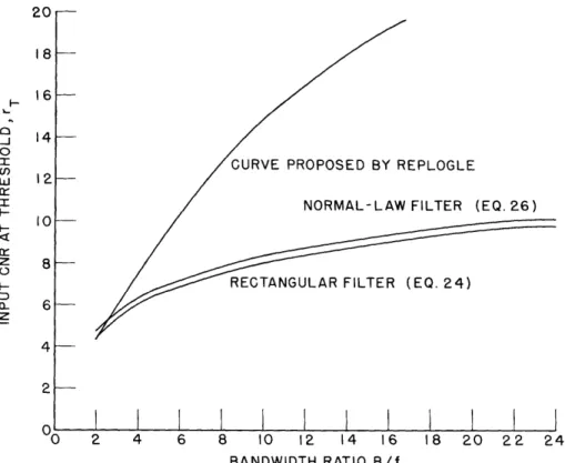
Both Eqs. 24 and 26 have been numerically solved by the author; the result is plotted in Fig. 5. (The threshold curve by Reploglel2 is also shown for purposes of compari-son.) Our curves are believed to be quite accurate over the entire range of values rT 5; below this region, that is, near the origin, our simplified analysis yields only a rela-tively crude estimate of the location of threshold.
Perhaps the most significant result is the threshold curve derived from the sinusoidal-modulation case, as given by Eq. 18. Using Eqs. 18 and 7 [or (11)], we obtain for the threshold condition with a rectangular bandpass filter
f3
e -rBfa < Br a (27)
Then, from reasoning identical to that leading to EBr
Then, from reasoning identical to that leading to Eq. 24, we have
PROPOSED BY REPLOGLE
NORMAL-LAW FILTER (EQ. 26)
RECTANGULAR FILTER (EQ. 24)
l
I I I I I I I I I I I
Vo 2 4 6 8 10 12 14 16 18 20 22
BANDWIDTH RATIO,B/fa
Fig. 5. Noise threshold curves for an unmodulated carrier.
24 RECTANGULAR FILTER,(EQ.28) APPROXIMATION (31) APPROXIMATION (40) 24 13 20 18-16 14 12 10 8 6 4 2
,L
I-0 0 I U) w a I cr z 0 z 16 14 I-j 12 0 n I I 8 Z 6 o a_ 4 z 2 C' Vo 2 4 6 8 10 12 14 16 18 20 22 BANDWIDTH RATIO,B/faFig. 6. Noise threshold curve for a modulated carrier.
---~II--`- - ''
1
e2 T TB . (28)
Tf
It is interesting to note that in this case rT exceeds 5 for any value of f 2, and is
~~~~~~B
avery close to 10 for -f = 10. Thus, the widely held belief that approximately 10 db CNR a
is needed to pass the threshold in a conventional FM system finds confirmation.
In the sequel we shall use the solution of Eq. 28, shown in Fig. 6, as the location of the noise threshold in conventional FM systems. By itself, however, Eq. 28 does not facilitate a direct algebraic approach to the evaluation of the performance of such sys-tems, and some further approximations will be needed.
6. Performance Analysis of Conventional FM Systems
It seems reasonable to assume that no FM system can satisfactorily operate below its (impulsive) noise threshold, since a sharp performance degradation is immediately noticed both with regard to the noise output power and to the appearance of noise clicks. Thus the performance of FM systems at and above threshold, as well as the location of the threshold in terms of received signal-power and noise-power spectral density, is of great interest. Since the minimum output signal-to-noise ratio, say, Rmin' is usually specified for the system, it seems reasonable to compare Rmin with the performance of the system at threshold, denoted here by RT. Other quantities of importance that must be specified in advance are: the message bandwidth fa' the system noise figure or noise power density No. The principal unknowns to be determined in system syn-thesis are: the modulation index m for the signal design, the minimum carrier power C for the transmitter design, and the filter bandwidth B for the receiver design.
The filter design will always be a compromise between minimizing the message dis-tortion and obtaining the best noise filtering. Without entering the controversial area of nonlinear message distortion in linear FM systems, we shall confine our attention to the relation between the FM signal bandwidth and the filter bandwidth. Specifically, the maximum signal bandwidth will be considered to be determined by the modulation
D
index m = f-, where D denotes the maximum signal-frequency deviation with modu-a
lating frequency fa' For purposes of engineering, it appears that the Van der Pol-Carson formula for the signal bandwidth,
Bs 2fa(m+l), (29)
is accurate enough.
*For the sake of precision, (29) may be extended as proposed by Manayev 17 so that it will account for all sidebands with amplitude exceeding 1 per cent of the unmodulated carrier amplitude. Then Bs = 2fa(1+m+ 4m).
With large modulation index (m>> 1), the term 1 in Eq. 29 can be neglected. Assume as a first measure for relatively undistorted signal transmission that the bandwidths of the signal and the bandpass filter are equal: B = B. Note also from Fig. 6 that, for large B/f a, a fixed value is a good approximation for the threshold CNR in the range 7 fB < 17, which corresponds to a modulation index in the range 2.5 < m < 7.5. We
a
therefore take
rT : 10. (30)
With actual systems, usually the input-noise power density No is fixed, rather than the power of noise filtered by the bandpass filter. We then have
CT
rT = N B = 10, (31)
o
where CT denotes the value of signal power C at the threshold. It is sometimes con-venient to refer the CNR to the baseband width, fa' in which case we define
C B
ra Nfa - (32)
Observe that in the linear region the normalized signal-output power is
S = D2, (33)
and with (7) we arrive at the well-established formula for the output signal-to-noise ratio
RS = 3rBD 3 2 (34)
2f3 2 a
a
Thus, for the broadband FM system with nearly rectangular filters "matched" to the signal bandwidth (so that B = 2m), we have
a
3 ZB 3 2
R -m2r m r 2m,
2 3 2
a
and at the threshold with (31),
RT 30m3. (35)
The "zero-order" solution of our system problems will then be
(36a) (36b) (36c) 15 m = RT/30 CT = 20Nomfa B = 2mf a -_-·1111111_1 3 _
Such a system exhibits a well-known inherent limitation of output performance, if carrier-power and noise-power density are fixed. From (31) and (32), we find
C
ra = N f - constant, (37)
oa
so that the maximum value of
C C
m Nf C r f (38)
oaT oa
is also limited. Consequently, for the maximum value of output SNR, we have
R max 3 3 ( Nf C \) 0.0 3 ( Nf (39)
This bound may be exceeded only by decreasing the noise-power density or by increasing the signal power.
For other systems, in which the modulation index is not necessarily much larger than one, say m < 5, we must take into account two corrections. The first must account for the significant fall in the threshold curve (Fig. 6); the second must allow for the sig-nal bandwidth being larger than the full frequency swing 2D = 2mfa . In this case we use Eq. 29 without neglecting the unity term.
The transcendental character of the threshold equation (28) impedes a straightforward analytic approach. In looking for algebraic fits, it is convenient to select an expression leading to a manageable system analysis along the lines presented in Eqs. 30-36. We therefore suggest the following algebraic approximation for use in place of Eq. 28 in the
range
-
~ 8: a25B 2
r 25 B( a ) (40)
T - 32 fa B +
Hence, substituting Eq. 29, after simplification we have (m+2)2
25
_(41) rT 16 m + 1 ' which is valid with m 3.The threshold CNR measured in the baseband width fa according to (32) is
r 25 (m+2)2, (42)
ra,T =-8
and the (linearized) output SNR at threshold (34) becomes
R=3 -2 I 75 m2(m+2). (43)
RT m ra,T 16 (43)
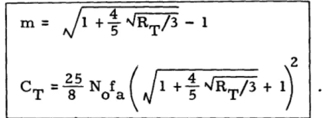
The following system equations follow immediately:
(44a)
(44b)
In addition, as usual, the filter bandwidth equals the signal bandwidth (29), so that
B = Zfa(m+l) = Zfa + 5 4RT/3 (45)
In order to represent all matched (B=Bs ) systems in the wide range of modulation indices by one graph, we combine both approximations: (35) for m > 3, and (43) for m < 3. In our plot the input is represented by ra, and the output R(ra,m) by a family
of straight lines with m as a parameter (Fig. 7). They are cut off by the threshold locus (36b) or (44b), respectively, for m <> 3.
The results, thus far, have been obtained under the assumption that the filters are
a-o z< w or 0 0. 60 55 50 45 40 35 30 25 20 15 In 10 INPUT ,T) r 15 20 25 30 35 40 CARRIER-TO-NOISE POWER RATIO,
(REFERRED TO BASEBAND)
45
ra (db)
Fig. 7. Performance of matched FM systems.
17 / 4 m =1 +(5 RT/3-1 CT Nofa 1 + -T-/ _ I I I I I I I , . j -I - I- -_ _ _ _ _ ! .v I
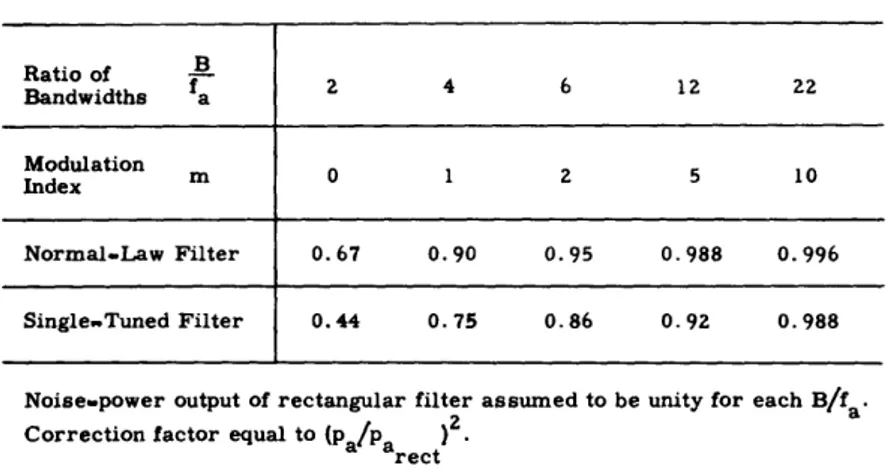
TABLE 2. Correction factor for noise-power output. Ratio of B Bandwidths fa 2 4 6 12 22 Modulation Modulation m 0 1 2 5 10 Index Normal-Law Filter 0. 67 0. 90 0. 95 0.988 0. 996 Single-Tuned Filter 0.44 0.75 0.86 0. 92 0. 988
Noise-power output of rectangular filter assumed to be unity for each B/fa. Correction factor equal to (pa/Pa )2
rect
nearly rectangular. As a final step, we should proceed to the general case for arbitrary filter shape. We have already investigated the noise-power output as influenced by the
bandpass filtering (section 2). With the matching of bandwidths, B = B, still assumed to be valid, we do not introduce any significant changes in the signal-output power. Thus,
modification of the gyration radius suffices to provide necessary correction terms for evaluating the output power of Gaussian noise, as well as the output SNR above the threshold.
Table 2 presents some results for cases of practical interest. Note that, in general, the correction factors are not very significant, except for the hypothetical limit B = 2,
a which corresponds to m - 0. Therefore, most conventional systems can be analyzed in accordance with (40), (41), (42), (43), and/or Fig. 7. For FM systems with a single-tuned bandpass filter, a check with the aid of Table 2 is recommended, since the cor-rection factor in some cases of small modulation index may be important.
18
PART B: FEEDBACK FM SYSTEMS 7. The Concept of Frequency-Compressive Feedback
The idea of a tracking FM system is not new; it originated, curiously enough, as a substitute for amplitude limiting in an FM receiver.18 But important noise-combating properties were soon noticed, 1 9'2 0 and some successful applications were reported.2 1 - 2 3 Later, realistic bounds on system performance were introduced2 4 ' 1 4 by taking into account the deficiencies inherently existing in a stable feedback loop.
The most important variety of a tracking FM system is the frequency-compressive feedback loop, which somewhat resembles a well-known feedback frequency-dividing scheme. In this report our interest will be strictly confined to the frequency-compressive FM demodulator as a device for decreasing the noise threshold in an FM system. Its mechanism is capable of reducing the bandwidth of threshold-causing noise without affecting the signal transmission and the output signal-to-noise power ratio. Thus an exchange between the power and the bandwidth of the input FM signal, or an increase in the usable range of a long-distance communication system with fixed signal power, is possible.
The frequency-compressive feedback loop of the usual type (see Fig. 8) has been looked upon either as a "frequency demodulator," 2 4'14 ' 2 5 or an "FM receiving
system." 2 ' 2 6 ' 2 7 Less customary varieties have sometimes been mentioned in the liter-ature, for instance, a loop without any amplitude limiterl8 or a loop driven from an amplitude limiter.l4 But these have been reported as being substantially inferior to their conventional counterpart.
Within the general structure of the frequency-compressive feedback loop (Fig. 8) some modifications are possible with respect to the location and the form of the output filter. It seems that it is most convenient to have the output filter independent of the
feedback filter; both can be connected across the output of the frequency demodulator.
AMPLITUDE AND ANGLE- MODULATED SIGNAL INI F SIGNAL 'UT
Fig. 8. Block diagram of a frequency-compressive feedback FM system.
19
Alternative arrangements introduce only a trivial difference in analysis and can be dis-regarded.
Even with the well-established form of the system under consideration, its analysis
presents many essential difficulties. These are due partly to the general complexity
of exponential modulation, which is a nonlinear transformation. Also, various
regen-erative phenomena exist within the loop, and affect its stability and the noise threshold
of the system. It is, therefore, easy to understand why the analysis of this system has
been less successful than its engineering applications, which were revealed in 1958,21
1960,2 2 and 1961.23 Important analytic progress by using linear approximations was
initiated in 1962. 2414
It seems advisable to point out again that the validity of the linear analysis, in which a baseband analog is utilized, is restricted to cases of approximately linear modulation. Small rms index angle modulation resulting from a useful message or a weak noise dis-turbance is nearly linear and can be rigorously treated with the aid of the linear model. On the other hand, the linear model is invalid for the analysis of the message distortion in a practical feedback system, because the I-F signal - in spite of the frequency
com-pression - is not small-index-modulated.
One more word of caution might be of use at the beginning of a study of this system. The noise threshold in the frequency-compressive feedback loop may be caused by two entirely different mechanisms: the conventional threshold, and the feedback threshold. Any system as a whole never exhibits more than one of these two noise thresholds. The question arises whether systems should be designed in which the feedback threshold
dominates. In our opinion, the answer is no, since in this case it has been found
experimentally that anomalies occur as a result of which the system performance is
sharply degraded. Furthermore, when the conventional threshold does dominate, the
behavior of the feedback system is, in fact, similar to the behavior of the same system
with open loop, that is, of a conventional system with a specific type of bandpass filter.
Therefore, an approach to the analysis of feedback systems, whereby the areas of validity of the conventional theory are determined and the feedback threshold is branded
as an anomaly to be avoided, is recommended here. This contention is largely backed
up by our experiments. Our analysis concentrates on the optimum design of the
feed-back filter and on the determination of the obtainable power-bandwidth trade-off. How-ever, an important area is still not covered by analysis: i.e., the regeneration of impulsive noise with strong feedback, although we have obtained some interesting experi-mental evidence regarding this phenomenon.
8. Noise Threshold in the Feedback System
It is now fully recognized that the random noise injected at the input to the frequency-compressive feedback loop (Fig. 8) can affect the system output in two different ways. Let us recall the normal behavior, common to all FM systems whether with or without
feedback. We shall consider the case in which the input consists of a carrier wave and
a band of Gaussian noise.
If the feedback system is above its noise threshold with the loop open and certain gain-phase conditions for proper noise tracking are met, then closing the loop will reduce both the output signal and the output noise in the same way, that is, by the compression factor F for the instantaneous values. Therefore, the output signal-to-noise power ratio remains unchanged as the feedback factor F increases from 1 up to a certain limit.
When the input carrier power is diminished, some excess terms of the output noise begin to appear in addition to the linear Gaussian term. Ultimately, the impulse excess noise (which appears as impulsive "clicks") predominates and produces a sharp noise in the noise output: the point at which this occurs is defined as the conventional threshold.
This threshold occurs at a specific value of the demodulator input CNR; it depends on the bandwidth B of the bandpass filter, but does not depend upon the feedback factor
F (at least not up to a specific value Fmax ; see section 11). On the other hand, since the frequency compression in the feedback system allows us to make the I-F filter nar-rower than it is in the conventional FM system with the same input signal, a reduction
of the threshold is possible. This is the main adavantage of the feedback system. From the argument above, we shall see that the conventional theory of noise in FM systems, specialized for the case of the single-pole filter with a relatively narrow band-width, is sufficient to predict the performance of the feedback system above the conven-tional threshold. This is obvious for small values of the feedback factor; it will be
shown, partly by experimental evidence, that the same type of behavior characterizes the frequency-compressive systems with stronger feedback. This occurs up to a cer-tain value Fmax , at which there is a rapid break of performance. Very pronounced bursts of impulsive output noise appear and at once degrade the message quality. The mechanism of this feedback threshold is not yet completely understood, but it appears that a cumulative action launches self-regenerating noise in the loop.
As in the conventional case, the precise definition of the threshold as a point rather than as a region is arbitrary: It can be approximately located as a specified departure from the linear input-output relation.
It should be clear from our description that any practical feedback system should not be brought up to the edge of breakdown; that is, the amount of feedback should be bounded by F max in order not to enter the detrimental region of the feedback threshold.
In other words, a well-designed frequency-compressive system will not exhibit the closed-loop threshold, since (by design) its conventional threshold predominates, simi-larly to the situation in a conventional system. Thus, a unified approach to all FM sys-tems appears to be justified.
At present, the bound imposed by the noise regeneration in the feedback loop is known and has been roughly determined by analysis. 24,14 Let us briefly recall Enloe's argument2 4 pertaining to the loop of Fig. 8, which is excited by a carrier wave and a band of weak Gaussian noise with spectral power density equal to No. After the band-pass filtering, the noise n(t) becomes narrow-band and can be represented by two
21
orthogonal components, say, nc(t) and ns(t).
Enloe's fundamental result, shows that the phase of the resultant wave at the fre-quency demodulator is
t) [s(t)-D(t)] - n(t I, (46)
where (t) denotes the phase fluctuation (caused by the input noise, and normalized by the carrier amplitude) of the feedback oscillator output. The circumflex stands for the filtering operation in the I-F path (that is, for convolution with the bandpass filter impulse response). Observe that the bracketed term denotes the quadrature noise com-pressed by the feedback action, and that the last term is excess noise derived from the in-phase component of input noise. Enloe24 presents arguments substantiating the fact that this last term is the most significant among second-order terms, and that the fluc-tuation of the envelope of demodulator input wave, which produces additional zero crossings, is negligible in the region of interest.
Under these conditions, it is the mean square of the VCO phase, 2(t), which deter-mines the significance of the additional noise component, and hence the closed-loop
1 2
threshold. Enloe has observed empirically that threshold occurs when g > _ 31 rad2, which we may approximate by the condition (D2 1/10 rad2. This is equivalent to the con-dition that the normalized mean square of the oscillator phase (caused by noise) is no longer small compared with unity. Enloe succeeded in translating this condition into a corresponding carrier-to-noise power ratio at the mixer input, whereby the amount of noise is determined by the closed-loop noise bandwidth. This makes the feedback
thresh-old dependent on the feedback factor. Thus, the noise threshthresh-old of the system can be degraded by the feedback action. The primary objective of our analysis is to describe the different consequences - positive as well as negative - of feedback in the loop.
9. Analysis of the Feedback Threshold
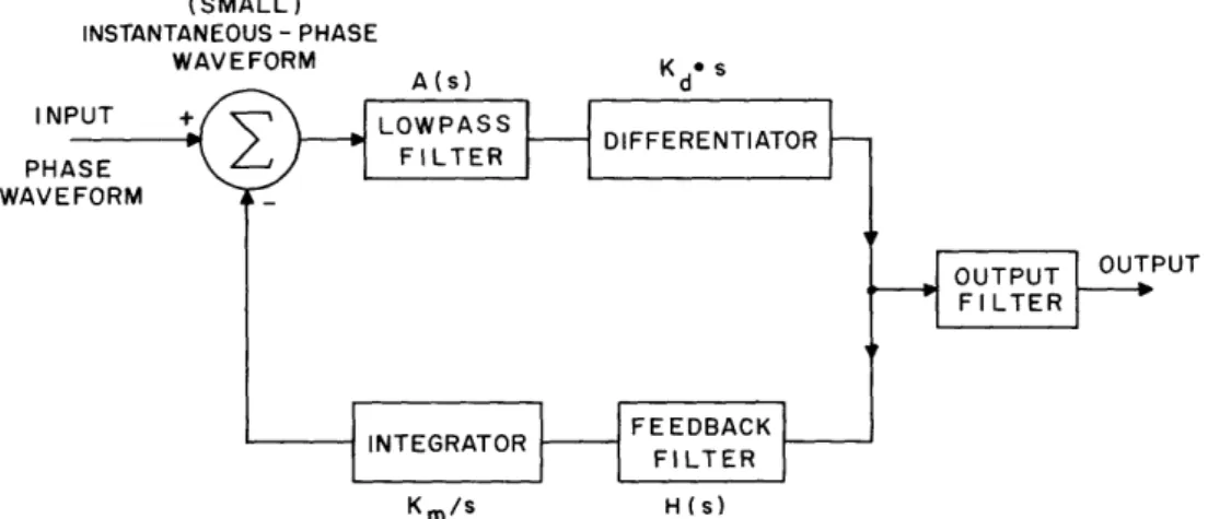
The linear analysis of a compressive-feedback FM system is based upon a conven-tionally constructed baseband analog. Transforming the system in Fig. 8, we make the following substitutions:
A phase and/or frequency subtracter replaces the mixer; A lowpass (analog) filter replaces the bandpass filter; A differentiator replaces the frequency demodulator; and An integrator replaces the variable oscillator.
We assume that our original FM signal is represented by its instantaneous phase as a time function, and that the input Gaussian noise is already narrow-band filtered. Thus it can be represented by its in-phase and quadrature components referred to the carrier frequency fc; that is
n(t) = nc(t) cos wct - n (t) sin ct . (47)
The linear baseband model shown in Fig. 9 is valid when the composite angle mod-ulation (by message, noise or both) is characterized by a small modmod-ulation index (rms).
This enables us to represent an exponentially modulated wave by the modulating wave (cf. Eq. 5 in Part A). Specifically, we can use the linear model for the analysis of the weak noise disturbance and for determining the border of the linear weak noise region.
Following Enloe's argument, we shall write the open-loop transfer function of the model in Fig. 9 as
Ho(s) = KdKmA(jw) H(jo), (48)
and then define the closed-loop transfer function for the transmission from signal input to the oscillator output
Ho(s)
Hc(s) = (49)
1 + Ho(S)
Note that this will reduce to the usual input-output closed-loop transfer function, as defined in linear feedback theory, only if the feedback filter is also used as the output filter.
The feedback factor F, as usual, is related to the loop gain at the lowest frequencies; then with A(O) - H(O) 1 we obtain
F 1 + H (0) = 1 + KdK, (50)
and we immediately find that
H (0) = F- 1 (51)
c = F
The two-sided noise bandwidth Bc of the closed loop is defined in the usual way, with the squared magnitude at the origin taken as the reference level:
1/z2rj jco
Bc
3(O)12
jo Hc(s) Hc(-s) ds. (52)Substituting (50) and (51) in (52), we have
F2 ]KdKmA(jw) H(jw)
B (F 2= & d m i |df. (53)
c _F- T -)o 1 + KdKmA(jw) H(jw)
The main finding of Enloe determines CF, the carrier power at the mixer input below which the noise regeneration in the loop begins to degrade performance:
NB C = o c F-1)2 2 23 ___
-11111-1---···111·111---(SMALL) INSTANTANEOUS - PHASE WAVEFORM K. s INI PHI WAVE PUT Km/s H (s)
Fig. 9. Linear baseband analog of the frequency-compressive feedback system.
Z
We have found it convenient to use the defining value = 0.1, and to refer the input carrier-to-noise power ratio at this "feedback threshold" to the baseband width fa. Then obviously A CF (CNR)f = Pa Nf '(55) a oa or B P= 5
LL
2 C(56) aEquation 56 locates the feedback threshold for a fictitious system without any conven-tional threshold. The structure of this expression resembles somewhat the structure of Eq. 32 in Part A.
In every real system, of course, the threshold occurs because of the mechanism that requires the higher value of comparable input CNR, measured at the same point and in the same bandwidth. With the linear model, transfer of the CNR from mixer input to demodulator input is straightforward, provided that the filtering is taken into account and a fixed reference bandwidth (preferably fa) is conserved. Under these conditions,
we can compare the effects of the two threshold-causing mechanisms on a frequency-compressive feedback system.
We have shown (section 5) that the conventional threshold of an FM system ra T defined in terms of the demodulator input CNR in the baseband, depends uniquely on the noise bandwidth of the (broader) bandpass filter, B, normalized by the baseband width.
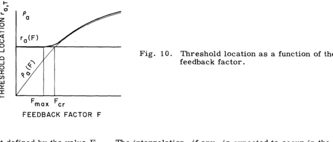
On the other hand, the feedback threshold Pa depends primarily on the feedback factor F, its dependence on B being of quite secondary importance. These very slightly inter-related effects can be visualized by referring to Fig. 10, which shows also the crossover
I-o J_ Z 0 0 _J -j I Cn I cr X ra (F) m :
Fig. 10. Threshold location as a function of the feedback factor.
Fmax Fcr
FEEDBACK FACTOR F
point defined by the value Fcr. The interrelation, if any, is expected to occur in the
vicinity of this crossover.
The actual noise threshold in the system is found experimentally to be nearly
inde-pendent of the feedback factor up to a value Fmax < Fr. From Fmax on, the feedback
begins to degrade the actual threshold; with F = Fcr the system threshold is exclusively controlled by the excess closed loop noise that causes bursts of clicks in the output. We consider this threshold to be different from the normal behavior of FM systems, and
much evidence for this claim will be shown. It was also predicted by an interesting
analysis of Baghdadyl4 (see his Eq. 111).
The main implication of this argument is a recommendation to design and operate
the feedback system in the region F < F ma x where the threshold is not degraded by
feed-back. In order to establish a proper setting for Fmax = c Fr, the crossover Fcr of
the two functions Pa and ra must be examined. Of particular importance is the
depend-ence of the feedback threshold on the parameters of the feedback filter, and this will be discussed first.
10. Analysis and Catalog of Feedback Filters
It has been concluded by independent investigators1 4 ' 2 7 ' 2 8 that the bandpass filter
in the feedback loop cannot have more than one pole, for stability reasons. In order
to obtain a stable feedback loop with finite noise bandwidth, it is then necessary to inter-relate the number of poles and the number of zeros in the transfer function Ho(s), for
the loop consisting of the two filters (shown in Figs. 8 and 9). In compliance with linear
feedback theory, we can envisage two alternatives: the number of poles exceeds the
number of zeros by one (this gives a better stability margin), or by two (this still gives
stability, although with a smaller margin). Here, the chain of broadband amplifiers
is not taken into account, mainly because it really should be avoided inside of the loop: otherwise, the parasitic time delay tends to destroy the stability of the system and proper
noise tracking. Accordingly, it seems desirable to have high gain in the stages before
the loop mixer.
25
`---Nonsingular zeros are not desirable in the bandpass filter. As for the low-pass feed-back filter, its zeros play an important role either in canceling the bandpass filter pole (the "canceling" zero) or stabilizing the feedback loop without increasing its noise band-width (the "stabilizing" zero). Practical considerations with respect to parasitic circuit elements show that the accuracy of the cancellation is always poor, and that attempts to cancel usually cause the appearance of some spurious time delays, with the deleterious effect just discussed.
It seems, therefore, reasonable to recommend no more than one canceling zero; thus the total number of poles around the loop seems to be restricted (in actual engineering implementation) to no more than three. Accordingly, the following structures of the feedback filter can be envisaged: 1 pole; 1 pole and 1 zero (stabilizing); 2 poles and
1 zero (canceling); 2 poles, 1 canceling zero and 1 stabilizing zero.
We note that all of these cases can be described by one general type of the open-loop transfer function:
Ho(s) = (F-1) X a X bX s + c (57)
o s+a s+b c
where a is the complex frequency of a pole in the feedback filter, b is the complex fre-quency of a pole in the bandpass filter analog or in the feedback filter, and c is the com-plex frequency of the stabilizing zero in the feedback filter. (There is no need to account for the canceling zero located at cIF, as long as it coincides with the pole of the I-F fil-ter.) In practical calculations it may be convenient to normalize a, b, c, as well as s, the baseband width a = Z2rfa.
a a
For the closed loop, we consider the transfer function (49) between the two inputs of the mixer:
H (s)
Hc(s) =
1 + Ho(S)
With some algebraic manipulation we obtain from (57) the general expression for the closed-loop transfer function:
ab(F-1)(s+c)/c
Hc(s) = (58)
2
~
ab(F-1)s +
a+
b + - s + abFThe closed-loop noise bandwidth Bc defined by (53) is presented below in a form that stresses the influence of the zero in the feedback filter, and is easily reducible to the no-zero case: ab 2 B= F c + abF B _ X (59) c 2(a+b) 2 abc c + (F-b ) a +b 26 ___ ___
It is easy to see from the denominator of (59) that with F
c > F -l (a+b)
the zero added in the loop for stability can also diminish the closed-loop noise bandwidth, and thus reduce the feedback threshold. More interestingly, it appears that for any given value of the feedback factor F there is one position copt of the stabilizing zero which produces a minimum in the noise bandwidth.
Differentiating (59) with respect to c, we find this optimum value to be
Copt = F [a+b+/a2+bZ+ab(F+ )1. (60)
Copt -F - 1
The corresponding minimum of Be is abF2 B cmin (F-1)cp t abF (61) a + b +/ a+b+ab(F+)
This simple but general result is of considerable interest in feedback-system syn-thesis. Observe that a minimum always exists for any choice of a and b in the left half-plane. The independent choice of a and b is secured only with the "2 poles and 2 zeros" structure of the feedback filter, so this class is expected to be the most prom-ising one.
Further investigation of the minimum-noise-bandwidth feedback loop can be carried out by perturbing - for a fixed value of F and with an optimum zero located by (60). In this optimizing procedure, necessary constraints must be established from bandwidth consideration of the open loop, which has to provide for nearly uniform feedback over the entire baseband.
Let us consider a family of different two-pole open loops (57) with the optimum zero (60), requiring first that the open-loop noise bandwidth be kept fixed. If the closed-loop
a a
noise bandwidth (61) is minimized as a function of , an optimum value of a = 1 can be found. This defines the so-called binomial filter: its simplest realization calls for two cascaded, real poles a = b.
For the binomial filter with (negative) real poles we obtain
copt a F + (62)
and
27
____. _
---B = a - (63) cmin (-F+ 1 )2
Note that for large values of the feedback factor F the noise bandwidth increases only proportionally to the square root of F; without the (optimum) zero it would increase proportionally to F, as shown in Table 3.
Another possible optimization procedure would call for a fixed half-power bandwidth of the open loop. We then rigorously find that the Butterworth filter with = j exhibits a minimum value of the noise bandwidth. Besides being maximally flat in frequency response, this filter also has the remarkable property of smallest possible noise
band-width with a second-order transfer function of fixed half-power bandband-width (in particular, smaller than the noise bandwidth of a binomial filter with equal half-power bandwidth).
The second-order Butterworth filter has two conjugate poles:
A A
a = A (l+j) b = (l-j).
It then follows that
c opt
(
F÷FNf N) (64)and
B
AF
(65)Cmin ,/F 2+1 + NZ
Again, for large F the noise bandwidth increases proportionally to
NI.
There is considerable numerical evidence for the superiority of the Butterworth filter over the binomial filter in the feedback path. This writer, for instance, has evaluated the frequency compression of the FM signal, under the assumption that the post mixer rms modulation index remains smaller than unity. The message compression factor at the highest modulation frequency fa was compared for the two above-mentioned filter types with optimum stabilizing zero and equal noise bandwidth. The difference was immaterial for lower values of feedback factor F; however, the advantages of the Butterworth filter were clearly shown for F > 5. They are attributed mainly to the fact that the optimum stabilizing zero for the Butterworth filter, as located by Eq. 64, is much closer to the poles than for the binomial filter (Eq. 62). Therefore, it seems justified to claim that the maximally flat feedback-filter response leads to the minimum of the closed-loop bandwidth.
We thus consider our survey of feedback-filter types to be completed and list the appropriate entries in Table 3.
11. Synthesis of the Feedback System
For the synthesis of a feedback FM system we have to specify the quantities that we shall consider as given: the message bandwidth fa' the lowest value of output
28
--signal-to-noise ratio RT, and the noise figure or the noise power spectral density No. Then the following characteristics of the system are still to be found: the (lowest) car-rier power CT, the signal modulation index m, the feedback factor F, and the bandwidth B of the I-F filter. Also, after some additional assumptions have been made, the struc-ture of the feedback filter and its parameters have to be chosen.
For practical calculations it is convenient to establish the input CNR as a measure of the carrier power CT; we will use the value at threshold, referred to the baseband
width
CT ra, T N f
-oa
(66)
A very general method of synthesis results if one assumes that the linear model is valid for the (not narrow-band) signal transmission, as well as for the noise filtering.2 9
One obtains two threshold equations in terms of the closed-loop transfer function, under the constraint that the bandpass filter width is matched to the (not fully compressed) I-F
signal at the highest baseband frequency. After Hc(j a ) has been found, we next deter-mine the open-loop transfer function, break it down into two factors, and synthesize the feedback filter from its transfer function.
A more careful approach, however, restricts the validity of the linear model (even for the compressed post-mixer signal) to the evaluation of weak noise-processing only.
Table 3. Catalog of feedback-filter structures. Filter Structure
Case Filter Type Poles Zeros Clcsed-Loop Noise Bandwidth Remarks
1 Ip a - -z} n General 2 bF c 2+ abF Expressions 2 lp - z(st.c a a IF c 4aF 4 2p- Iz(c) aF binomial aI 2, IF A Zp - lz(c) a1 (l AF Buttrwotha * A cIF Butterworth a1 F(l-j) F Noise bandwidth
S 2p ·-
~z
Cope aF--F minrniedbinomial aI m 2a IF
6 Zp-Zz IY 2 opt
AF4'-Butterworth a2' _ (l"Ij) CIF +
29