HAL Id: hal-03231513
https://hal.inria.fr/hal-03231513
Submitted on 20 May 2021
HAL is a multi-disciplinary open access
archive for the deposit and dissemination of
sci-entific research documents, whether they are
pub-lished or not. The documents may come from
L’archive ouverte pluridisciplinaire HAL, est
destinée au dépôt et à la diffusion de documents
scientifiques de niveau recherche, publiés ou non,
émanant des établissements d’enseignement et de
Biophysics-based statistical learning: Application to
heart and brain interactions
Jaume Banus, Marco Lorenzi, Oscar Camara, Maxime Sermesant
To cite this version:
Jaume Banus, Marco Lorenzi, Oscar Camara, Maxime Sermesant. Biophysics-based statistical
learn-ing: Application to heart and brain interactions.
Medical Image Analysis, Elsevier, 2021, 72,
Biophysics-based Statistical Learning: Application to Heart
and Brain Interactions
Jaume Banusa,∗, Marco Lorenzia, Oscar Camarab, Maxime Sermesanta
aUniversit´e Cˆote d’Azur, INRIA Sophia Antipolis, Epione Project-Team, France bPhySense group, BCN-MedTech, Department of Information and Communication Technologies,
Universitat Pompeu Fabra, Barcelona, Spain
Abstract
Initiatives such as the UK Biobank provide joint cardiac and brain imaging information for thousands of individuals, representing a unique opportunity to study the relation-ship between heart and brain. Most of research on large multimodal databases has been focusing on studying the associations among the available measurements by means of univariate and multivariate association models. However, these approaches do not pro-vide insights about the underlying mechanisms and are often hampered by the lack of prior knowledge on the physiological relationships between measurements. For in-stance, important indices of the cardiovascular function, such as cardiac contractility, cannot be measured in-vivo. While these non-observable parameters can be estimated by means of biophysical models, their personalisation is generally an ill-posed prob-lem, often lacking critical data and only applied to small datasets. Therefore, to jointly study brain and heart, we propose an approach in which the parameter personalisation of a lumped cardiovascular model is constrained by the statistical relationships ob-served between model parameters and brain-volumetric indices extracted from imag-ing, i.e. ventricles or white matter hyperintensities volumes, and clinical information such as age or body surface area. We explored the plausibility of the learnt relation-ships by inferring the model parameters conditioned on the absence of part of the tar-get clinical features, applying this framework in a cohort of more than 3 000 subjects and in a pathological subgroup of 59 subjects diagnosed with atrial fibrillation. Our
∗Corresponding author: Tel.:+0-000-000-0000
results demonstrate the impact of such external features in the cardiovascular model personalisation by learning more informative parameter-space constraints. Moreover, physiologically plausible mechanisms are captured through these personalised models as well as significant differences associated to specific clinical conditions.
Keywords: Lumped model, Cardiovascular modelling, Personalisation, White matter damage, Atrial fibrillation, Heart-Brain interaction
Glossary: τ: Arterial compliance, σ0: Contractility, C1: Stiffness, R0: Left
ventri-cle radius, Rp: Peripheral resistance, AF: Atrial fibrillation, BSA: Body surface area,
CO: Cardiac output, DBP: Diastolic blood pressure, EDV: End-diastolic volume, EF: Ejection Fraction, ESV: End-systolic volume, GM: Grey matter, IUP: Iteratively up-dated priors, MBP: Mean blood pressure, SBP: Systolic blood pressure, SV: Stroke vol-ume, WM: White matter, WMHs: White matter hyperintensities.
1. Introduction
Heart and brain are linked by pathophysiological and physiological mechanisms sharing several risk factors (Doehner et al., 2018). For instance, despite the heteroge-neous clinical manifestations of cerebrovascular diseases and cognitive decline, clin-ical evidence supports a common underlying cardiovascular pathophysiology relating cardiac function and brain damage (Moroni et al., 2018). Moreover, there is a vari-ety of heart diseases such as heart failure (HF) (Ois et al., 2008) or atrial fibrillation (AF) (Benjamin et al., 2018) that are considered independent risk factors for demen-tia (Chen et al., 2018; Alonso and Arenas de Larriva, 2016) and have been related to cerebrovascular diseases, doubling the risk of dementia (Azarpazhooh et al., 2018).
Nevertheless, the lack of databases integrating heart and brain data of the same sub-jects has prevented to study their relationship in depth, in particular through advanced modeling tools. Current initiatives providing systemic databases of both heart and brain imaging information, such as UK Biobank (Sudlow et al., 2015) or the Heart-Brain study (Hooghiemstra et al., 2017), have the potential of improving our understanding by means of large-scale data analysis. From cardiac imaging data it is possible to obtain
volumetric indices characterising cardiac function, such as stroke volume (SV), cardiac output (CO), end-diastolic volume (ESV) or end-systolic volume (EDV). From brain imaging we can obtain indices related to the main structures present in the brain, sub-cortical regions, or pathological indices such as white matter hyperintensities (WMHs). WMHs are a common marker of brain damage associated to dementia, cognitive de-cline and risk of stroke (Wardlaw et al., 2015) and can be measured as hyperintense regions in T2-weighted magnetic resonance images (MRI). Although the pathogenesis of WMHs remains unclear, current hypotheses suggest a vascular origin, supported by the association with elevated blood pressure (Modir et al., 2012; Moroni et al., 2018), brain hypoperfusion (Jefferson et al., 2009) and cardiac pathologies such as HF (Alosco et al., 2013) or AF (Alonso and Arenas de Larriva, 2016).
The link between cardiovascular risk factors and brain imaging changes is com-monly studied by means of multivariate regression analysis or proportional hazards models (Debette and Markus, 2010; Friedman et al., 2014). However, there are sev-eral descriptors of the cardiac function that are not possible to obtain in-vivo such as cardiac fiber contractility or stiffness among others, thus limiting the hypotheses that can be tested, along with the interpretation of the results. Cardiovascular biophysical models allow to estimate these descriptors through data assimilation procedures and provide mechanistic insights of the cardiac function that can help us to better under-stand its effects on the brain.
To tackle this problem, we propose an approach in which we combine the person-alisation of a biophysical model, deriving non-observable parameters, with statistical learning to link cardiac function to brain damage using indices extracted from imaging data available in UK Biobank. We represent the interaction between the brain state and cardiac function by constraining the space of feasible solutions of the model. Our ap-proach extends the work described in (Moll´ero et al., 2018) and our preliminary work presented in (Banus et al., 2019) and is based on a group-wise regularisation term pa-rameterised by a covariance matrix that takes into account the relationships between model parameters (e.g. contractility) and external indices not present in the model, such as brain volumetric indices (e.g. WMHs).
subjects for which cardiac and brain information is jointly available in the UK Biobank database, identifying statistically significant associations between the personalised model parameters and brain volumetric features that match findings reported in previous clin-ical studies. Next, we explored the plausibility of the learnt relationships by inferring the model parameters conditioned on the absence of part of the target clinical features. Finally, we applied the developed framework in a subset of subjects diagnosed with AF, demonstrating the ability of the framework to identify significant differences as-sociated to clinical conditions. To our knowledge, no patient-specific modelling study relating brain damage and cardiovascular parameters has been done before, and this study presents the largest cohort of personalised subjects to date.
The paper is structured as follows. Section 2 introduces the context of our work and Section 3 introduces the methodological framework, describing the biophysical model, the personalisation approach and how we combine it with group-wise regularisation. Next, in Section 4 the framework is applied to brain and heart data, first using the whole cohort and then in a subset of subjects diagnosed with AF. We detail the data pre-processing and inclusion criteria and examine the obtained results and the plausibility of the model based on the learnt relationships. Finally, in Section 5 the limitations of our framework and possible future directions are discussed and in Section 6 we summarise the conclusions of our work.
2. Methodological context
Usually the association between cardiac imaging indices and vascular risk factors (VRFs) such as hypertension, diabetes, smoking, obesity or hyperlipidemia with brain imaging features is studied by means of standard statistical tools such as multivari-ate regression or survival analysis models. Following these analyses, cardiac output and reduced brain blood flow have been associated to greater WMHs burden (Jefferson et al., 2009; Bahrani et al., 2017), while a review of 46 longitudinal studies associated WMHs with a higher risk of dementia (Debette and Markus, 2010). Moreover, based on a meta-analysis of 77 studies VRFs were found to be independently associated with brain imaging changes even before the clinical manifestation of cardiovascular or
cere-brovascular diseases (Friedman et al., 2014). More recently, studies based on the UK Biobank have supported these findings. In (Veldsman et al., 2020) cerebrovascular risk factors were associated with reduced cerebral grey matter and white matter integrity, and in (Cox et al., 2019) hypertension was independently associated with generalised atrophy of the brain (reduced brain volume and thinner cortex) and a higher burden of WMHs, while increased pulse pressure was related to poorer white matter measures.
The use of cardiovascular models enables to study the effect of cardiac function in the brain from a mechanistic perspective, and allows to introduce prior knowledge on the physiological links between the available measurements. For example, (Scarsoglio et al., 2017) studied the effect of AF in brain perfusion and determined that the loss of periodicity in the AF beat-series leads to a higher occurrence of hypoperfuse and hypertense events in the distal regions of the cerebrovascular circulation (arterioles and capillaries). Additionally, (Aghilinejad et al., 2020) determined that the stiffening of the aorta relative to the carotid arteries increased the pulsatility of blood flow in the brain vasculature, leading to increased microvascular damage.
However, personalising a cardiovascular model for a given subject is an inverse problem that implies estimating the model parameters such that generate simulation results as close as possible to the available clinical data. Carrying out the personali-sation of such models is complex. This problem is commonly ill-posed and its com-plexity scales quickly with the number of parameters. Several approaches have been proposed for cardiac-related inverse problems. When sequential data is available, it is common to rely on filtering approaches such as the unscented Kalman filter (UKF) (Pant et al., 2017) that corrects the model based on the discrepancy between the in-put data and model’s prediction. Other options involve data-driven approaches such as reinforcement learning (Neumann et al., 2016), gradient-based approaches based on the adjoint method (Delingette et al., 2012) or gradient-free approaches such as ge-netic algorithms (Khalil et al., 2006). Moreover, multi-fidelity approaches, based for example on evolutionary algorithms (Moll´ero et al., 2017) or filtering approaches (Pant et al., 2014), have been used to combine the computational efficiency of reduced-order models with the accuracy of higher-order models. Personalisation is commonly carried out at most in tens or a few hundreds of subjects (Moll´ero et al., 2018). Hence,
typi-cally the approaches are oriented towards obtaining solutions that mimic the observed clinical features but they do not prioritise obtaining homogeneous solutions in groups of subjects. Therefore, due to the ill-posed nature of the problem, a large variability between solutions in similar subjects can be found. This is a problem if we wish to in-clude the estimated parameters in any post-hoc analysis with the other available clinical information, such as brain volumetric indices.
3. Methodological framework 3.1. Cardiovascular biophysical model
c) Active force Passive Force Myocardial forces (BCS) Left Ventricle Right Ventricle Right Atrium Veins Systemic Arteries Systemic Le Atrium Arteries Veins Pulmonary Pulmonary Available data a) b) N EDV ESV SBP DBP
Scheme of the lumped model
Pressure and volume curves
IUP
Age, BSA, Sex WM GM WMHs Ventricles SV EDV ESV EF DBP SBP MBP + Prior Fitting Error
Figure 1: Graphical scheme of the iterative updated priors (IUP) personalisation approach. Dashed lines represent which information is grouped across the N subjects to define the prior. a) Summary of the available data for each subject, including cardiac data, socio-demographic information, blood pressure measurements and brain volumetric indices. b) Simplified representation of the lumped model showing the parameters used in the personalisation (θ). C characterises the compliance of the main systemic arteries, Rpthe peripheral resistance, τ represents the characteristic time of the RC system, R0the radius of the left ventricle, σ0the contractility of the cardiac fibers and C1their stiffness. c) Example of the pressure and volume curves that can be obtained from the model. From these curves we extract scalar indices (e.g. EDV, ESV) to match the available clinical data (target features). Curves have been extracted from the model locations with the corresponding matching frames colours.
In our work the cardiovascular model is the joint contribution of two components: a lumped model simulating the haemodynamics of the vascular system relying on the
electronic-hydraulic analogy; and an electromechanical model of the heart (see Figure 1). In the lumped model pressure and blood flow curves are simulated at specific lo-cations of the cardiovascular system throughout the cardiac cycle. We can formalise a system of ordinary differential equations (ODEs) that defines the flow-pressure dy-namics at each of the represented compartments of the model; the systemic and pul-monary circulations are represented as a three-element Windkessel (RCR) model cou-pled to a venous return (RC). The modelling of the electromechanical behaviour of the heart is carried out by the Bestel-Clement-Sorine (BCS) model (Chapelle et al., 2012; Marchesseau et al., 2013). The sarcomere contractile forces are modelled as the sum of a passive non-linear elasticity and an active contraction in the fibre’s direction. The model is able to replicate the Starling effect and is compatible with the laws of thermodynamics. The 0D reduction of the joint model was derived in (Caruel et al., 2014). In short, the ventricle is treated as a 3D symmetric sphere in the 0D model, where the myocardial forces and motion can be described by the inner radius (R0) of
the ventricle. Deformation and stress tensors are also reduced to 0D forms, allowing to characterise the heart contractile (σ0) and elastic (C1) properties of the heart. Hence,
the joint model ψ consists of a set of ordinary differential equations with nψparameters
(e.g. maximum contraction of the heart fibers or its stiffness), while the state variables of the model are denoted by O (e.g. arterial or venous pressures). A scheme of the model is shown in Figure 1b.
3.2. Biophysics-based statistical learning
Formally, during the personalisation stage, a subset of nt state variables or target
featuresfrom the data, ˆO = ( ˆO1, ˆO2, ..., ˆOnt) are used to optimise a subset θ of the nψ
model parameters. We denote O(θ) the set of state variables generated by the model for a given set of θ. The goal is to find θ∗such that O(θ∗) best approximates the target
features ˆO. This optimisation procedure can be expressed as in Equation 1: dO
dt = ψ(θ, t), ˆ
O ← O(θ∗)
We carried out the personalisation through the evolutionary strategy CMA-ES (co-variance matrix adaptation evolution strategy), which is a gradient-free approach based on maximum likelihood estimate of the parameters (Hansen, 2016). At each itera-tion CMA-ES evaluates several candidate soluitera-tions and assigns to each one a score, in this case the personalisation error. Based on the score ranks, a subset of best per-formance solutions is used to update the sampling distribution of the parameter-space. This allows CMA-ES to explore the parameter-space while being robust to possible divergences leading to non-valid sets of parameters, in which the score can be arbitrary high. At the same times it makes CMA-ES well suited to parallel environments, since we can evaluate several solutions independently.
We denote as S (θ, ˆO, T ol) the error function that we want to minimise, defined as the L2 distance between O(θ) and ˆO. Since each target feature has different range of
values to compare the different outputs for each feature f a tolerance interval (Tol) is defined, which can be formalised as:
S(θ, ˆO, T ol) = nt X f=1 (Of(θ) − ˆOf)2 T olf (2)
Following the method of iterative updated priors (IUP) (Moll´ero et al., 2018) group-wise constraints can be introduced during the optimisation process to obtain consistent solutions at population level, tackling the identifiablity problem. In the IUP method a regularisation term, R(θ, µ,Σ), is used to reduce the variability in the estimation of the parameters. This regularisation constraints the directions in which the parameter-space is explored by leveraging on the relationships among model parameters. Formally, the estimated regularisation term is parameterised by an expected value µ and by a covariance matrixΣ encoding the relationship across parameters:
R(θ, µ,Σ) = (θ − µ)TΣ−1(θ − µ). (3)
Therefore, the error function becomes:
S(θ, ˆO, µ, Σ, Tol) = S (θ, ˆO, Tol) + γR(θ, µ, Σ), (4) where γ defines the relative weight of the regularisation term. This term is updated
at each IUP iteration using the obtained mean value of the fitted parameters and the estimated covariance in the previous iteration.
The regularisation term R(θ, µ,Σ) can be extended to incorporate features not present in the cardiovascular model. The extended feature space corresponds to the concate-nation of the model parameters, θ, with external features, φ, which represent other available subject’s information such as volumetric indices extracted from brain scans, or weight and height as in (Moll´ero et al., 2018). In this work, we incorporated volu-metric features extracted from brain images such as whole brain and ventricle volumes, WMHs features, as well as age and body surface area (BSA). Let µφandΣφdenote the
mean of the external features and their covariance respectively. Then,Σi,φcorresponds
to the cross-covariance between the external features and the model parameters. There-fore, the error function to be minimised in Equation 4 becomes:
S(θ, ˆO, µ∗, Σ∗, T ol) = S (θ, ˆO, Tol) + γR(θ, µ∗, Σ∗), (5)
µ∗= µi µφ , Σ∗= Σi Σi,φ Σφ,i Σφ . (6)
Equation 5 now accounts for a covariance term constraining the parameters accord-ing to the extended set of features.
By default CMA-ES initially samples solutions according to a standard multivariate Gaussian distribution, which is updated at each sampling iteration based on the best-performance solutions of the previous one, parameters are supposed to have similar sensitivity to properly explore the parameter-space in all directions. To promote this behaviour, we introduced for each subject s a mean and a covariance hyper-parameters, msi and Csi respectively, which are updated at each IUP iteration. These additional
hyper-parameters allow to account for the different sensitivity of the model parameters during optimisation, and promote a more accurate exploration of the parameter space through sampling. Both mean and covariance are computed using the sampled solu-tions of CMA-ES, ˆxs, at the iteration in which we get the optimal set of parameters θ∗s.
The individual mean and covariance are used to scale the solutions, ˆxs, into the actual
A scheme illustrating the personalisation of the cardiovascular lumped model with subject’s brain and heart data is shown in Figure 1; pseudo-codes for the IUP and the scaled CMA-ES are shown in Algorithm 1 and Algorithm 2 (in the Appendix), respectively.
Algorithm 1 IUP pseudo-code.
1: Inputs:
2: Nsubjects with nttarget features ( ˆO) and neexternal features (φ)
k ←IUP iterations T ol ←Tolerance interval C MAoptions 3: Returns: 4: θ∗, µ∗, Σ∗, C, m 5: Initialize: 6: Σφ, µφ← external features i ←0 7: 8: while i< k do 9: if i== 0 then
10: Initialise parameter prior covariance (Σi) and mean (µi) as null values
11: end if
12: µ∗i, Σ∗i ← Extend prior terms as in Equation 6
13: for s ← 1 to N do
14: θ∗si, Csi, msi← Scaled-CMA(C MAoptions, T ol, µ∗i,Σ ∗ i, Csi, msi) 15: end for 16: µi+1← mean of the {θ∗si}Ns=1 Σi+1← covariance of the {θ∗si}Ns=1 i ← i+ 1 17: end while
T1 and T2 images (5394)
Features derived from cardiac images
(4424) Incompatible or unsusable T1 or T2 (710) Overlapping data (3564)
Blood pressure, age, height or weight not
available (65) WMHs segmentation failed (54) Quality control WMHs segmentation Included subjects (3445) UK Biobank
Figure 2: Schematic representation of the inclusion criteria used in our study.
a) FAST Segmentation b) T1 c) T2 FLAIR
WM
GM
Brain
ventricles WMHs
Figure 3: Example of the available brain volumetric information for each subject. a) Segmentation of the main brain tissues, white matter (WM), grey matter (GM) and brain ventricles using the FAST algorithm of FSL (Zhang et al., 2001). Image processing was carried out using the pipeline described in (Alfaro-Almagro et al., 2018). b) T1 sequence and c) T2 FLAIR MRI sequence with WMHs segmentation overlaid, carried out using the LPA toolbox for SPM
4. Application to brain and heart data 4.1. Clinical data and pre-processing
The UK Biobank database provides demographic information (e.g. age, sex, height or weight) and clinical measurements such as brachial blood pressures (both diastolic and systolic; DBP and SBP respectively), image-derived features from both brain and cardiac MRI, clinical diagnoses and several MRI modalities of the brain.
For our analysis we selected a subset of subjects for which brain T1 and T2 FLAIR MRI modalities were labelled as usable for segmentation and all cardiac-image derived indices were available, for a total of 3564 subjects (see Figure 2). The cardiac indices were extracted from the segmentation of the left ventricle in short-axis cine images, including SV, EDV, ESV, CO and EF. Using T1 and T2 FLAIR MRI, WMHs were segmented using the lesion prediction algorithm (LPA) (Schmidt, 2017), available in
the lesion segmentation toolbox (LST) of SPM1. From the resulting segmentations we
extracted the total volume of WMHs and number of lesions. Other volumetric in-dices such as the total grey matter (GM), white matter (WM) and brain ventricles vol-umes were obtained from the T1 MRI according to the protocol described in (Alfaro-Almagro et al., 2018). All brain-related volumes (including WMHs) were normalised by head size. The WMHs total volume and number of lesions presented a positive skewed distribution; in order to obtain a more suitable distribution for our statistical approach we used the Box-Cox transformation to normalise the distributions.
According to (Ribaldi et al., 2018) the obtained WMHs volumes using the LPA are comparable to the ones obtained through manual segmentation. Nevertheless, for each subject the segmentation of WMHs was visually assessed and the non-acceptable ones were excluded. Moreover, subjects for which one of the demographic features of interest (age, sex, height or weight) or blood pressure were not available were also dis-carded. The final number of available subjects was 3445. Height and weight were used to compute the body surface area (BSA) of each subject according to Mosteller for-mula (Mosteller, 1987): BS A=
q
Weight[kg]∗Height[cm]
3600 . Summary statistics of the dataset
are provided in Table 1, and Table A.2 in the appendix provides the corresponding data-field codes from the UK Biobank.
We used as target features EDV, SV, EF, MBP and DBP. ESV was discarded from the volumetric features since it did not provide additional information concerning the selected features. While, among the available pressure information MBP and DBP were used since we did not have pressure information at the aorta level, and unlike SBP, both MBP and DBP exhibit similar values in the main systemic arteries (Muiesan et al., 2014). Based on previous experience (Moll´ero et al., 2018) and on the available data, the most sensitive parameters were selected to enter the personalisation procedure: the contractile and elastic behavior of the left ventricles (σ0, R0, C1) and parameters
related to the systemic vasculature properties (Rp, τ). Moreover, heart rate information
obtained during the cardiac MRI was used to determine the heart period of the model for every subject. For the volumetric features (SV, EDV) we set a tolerance interval
Table 1: Statistics of the analysed UK Biobank dataset, including AF and control subjects. Bold features are significantly different between AF and a randomly sampled representative control group (two-sample t-test, p ≤ 0.05) when Bonferroni correction is not applied. The control group was sampled to match on Age, Sex and BSA. The volume of WMHs and the number of WMHs were normalised using the Box-Cox transformation.
UK Biobank Atrial Fibrillation Sample Control
Subjects (M/F) 1555/1890 45/14 42/17
Mean ± Std Mean ± Std Mean ± Std
Age (Years) 61.07 ± 7.12 65.79 ± 6.86 64.54 ± 4.62 BSA (m2) 1.88 ± 0.21 2.02 ± 0.20 1.97 ± 0.17 DBP (mmHg) 75.49 ± 12.10 75.67 ± 12.29 77.64 ± 12.69 SBP (mmHg) 132.09 ± 18.77 133.15 ± 19.52 139.12 ± 20.34 MBP (mmHg) 94.35 ± 13.12 94.83 ± 13.30 98.13 ± 13.84 SV (ml) 77.58 ± 17.70 76.08 ± 20.65 77.1 ± 18.77 EDV (ml) 138.95 ± 32.6 152.86 ± 32.84 142.96 ± 33.23 ESV (ml) 61.37 ± 19.85 76.72 ± 25.81 65.79 ± 19.46 EF (%) 56.21 ± 6.24 50.28 ± 10.16 54.23 ± 7.74 WM (mm3) 711,454 ± 40,719 701,887 ± 43,838 711,360 ± 46,615 GM (mm3) 801,685 ± 46,702 763,876 ± 48,842 788,936 ± 43,348 Ventricles (mm3) 42,807 ± 17,612 55,103 ± 21,930 45,925 ± 16,705 WMHs (a.u) 7.5 ± 2 8.64 ± 2.12 7.51 ± 1.91 # WMHs (a.u) 3.27 ± 0.85 3.73 ± 0.83 3.41 ± 0.79
of 10 ml, 200 Pa for pressures (MBP, DBP), and 5% for the EF, based on the clinical uncertainty of these values. This tolerance interval was used to assess the convergence of the model. As initial values for the varying parameters we used the model default values (see Table B.3 in the Appendix). After personalisation we used the Spearman’s rank coefficient to study the associations between the estimated model parameters and
the external features. The number of IUP iterations and the hyper-parameters of the CMA-ES algorithm were determined empirically as: population size (20), number of iterations (100), initial variance (0.1) and 5 IUP iterations. We applied the framework to the available UK Biobank cohort and used the results to assess the model plausibility, next we applied the framework to a subgroup of subjects diagnosed with AF.
4.2. UK Biobank
We run our framework in the whole available cohort (3445 individuals) and studied the associations between external features, target features and varying model parame-ters, as well as the parameter’s distribution at each IUP iteration, convergence rate and error between the target features and the simulations. We also considered five regular-isation levels γ= (0.1, 0.5, 1, 2, 10), and the presence or not of the external features in the regularisation term.
4.2.1. Model plausibility
To assess the influence of the external features included in the covariance matrix of our prior we simulated a scenario in which only DBP and MBP were available while inferring all the varying parameters, i.e. where the volumetric information was miss-ing (SV, EDV, EF). Hence, we selected a subset of 100 random subjects and run one IUP iteration using as regularisation term the final prior learnt in the whole cohort with and without external features. Then, we assessed the difference between the values of the estimated parameters for these subjects with respect to the ones obtained when all the target features were available, and the missing target features were compared to the model’s simulations. We measured the differences using the Mahalanobis dis-tance, DM(x, y)= p(x − y)TΣ−1(x − y), whereΣ represents respectively the covariance
matrix of the missing target features when compared to the simulated ones, and the covariance matrix of the estimated parameters with all the target features when the model’s parameters are compared.
In Figure 4a we observe the distance between the missing target features (EDV, EF, SV) and the ones simulated by the model. We observe that while regularisation helps to reduce the error for values of γ ≤ 1, the tendency changes when γ > 1. The
(b) Estimated parameters (a) Missing features
Figure 4: Mahalanobis distances between: a) missing features and simulated results of the model. b) the estimated parameters with missing features and the estimated parameters with all target features. * denotes that distributions are significantly different according to Wilcoxon rank-sum test using a significance level of α = 0.05
use of external features in the prior reduces this discrepancy, although not significantly. Figure 4b demonstrates that with an increased regularisation the distance between the parameter’s values estimated using a subset of the target features and the ones obtained using all of them is reduced. Moreover, in this case the difference is significant. Hence, the presence of the external features allows to learn a more meaningful representa-tion of the parameter-space. Based on these observarepresenta-tions, the results of the following sections were obtained by setting γ = 1 and using external features. Results at other regularisation levels and without external features can be found in the supplementary material.
4.2.2. Analysis of brain-cardiac relationship in the UK Biobank
Figure 5a shows an example of the parameter’s distribution at each IUP iteration of the cardiac contractility parameter (σ0). We can observe how at each IUP iteration the
distribution of the estimated parameters shrinks with increasing regularisation, reduc-ing the number of outliers and extreme values. The regularisation term penalises the exploration of certain directions in the parameter-space based on the available informa-tion. At the same time, the median absolute error as a percentage of the target features stays around 5% as can be seen in Figure 5b. Moreover, the majority of the studied subjects (90.39%) reached convergence according to our tolerance interval, T ol. Fi-nally, Figure 6 shows the Spearman’s rho correlations among the external features, the
(a) Distribution of across IUP iterations (b) Fitting errors
Figure 5: a) Kernel density estimate (KDE) of σ0(cardiac contractility) at each IUP iteration with external constraints and γ= 1. The rest of the parameter’s distributions are available in the supplementary material. b) Absolute reconstruction errors as a percentage of the target features values.
(a) Model parameters - Target features (b) Model parameters - External features (c) External features - Target features
Figure 6: Correlations heatmap between features and model parameters. The associations have been assessed by means of Spearman’s rank correlation coefficient and corrected for multiple comparison using the Bon-ferroni’s method. Non-significant correlations are considered as 0 (white). a) Associations between target features and model parameters b) relationships between the model parameters and the external features c) correlations between target features and external features.
model’s parameters and the target features. Several observations can be made from the figure:
1. Model parameters - Target features: We observe how the radius of the left ven-tricle, R0, is strongly correlated with the end-diastolic volume, slightly less with
the stroke volume, and negatively with the EF. The peripheral resistance, Rp,
is correlated with the pressure indices, DBP and MBP, and inversely related to the end-diastolic volume and the stroke volume. The compliance of the main arteries, τ, is closely related to the diastolic pressure, and affects in the opposite
way the systolic pressure, affecting the relationship between the mean and the diastolic pressure. The contractility σ0is strongly correlated with the EF and
in-versely with the end-diastolic volume and the stroke volume, while the stiffness of the heart, C1, affects negatively the EF and the end-diastolic volume and the
stroke volume.
2. External features - Target features: The relationship between target features and external features is mostly negligible. We only observe a strong positive associa-tions between the heart volumetric indices (EDV, SV) with BSA, and a negative one with respect to age.
3. Model parameters - External features: We observe how the left ventricle con-tractility, σ0, is positively correlated with brain volume and negatively with the
rest of volumetric indices, such as ventricles volume and WMHs. The same behaviour is observed in the relationships of C1. The radius of the left
ventri-cle, R0, is inversely related to age, WMHs volume and positively with BSA; for
the remaining indices it does not show any significant association. The periph-eral resistance, Rp, shows a positive association with WMHs volume, number
of WMHs, brain ventricles volume and age and negative with brain volume and BSA. The main arteries characteristic time, τ, which is proportional to the arte-rial compliance, shows the opposite relationships.
The results show an expected association between larger heart ventricles, R0, and
greater blood volumes such as the end-diastolic volume, EDV (Jegier et al., 1963). Also we observe how an increase in peripheral resistance, Rp, leads to an increase in
afterload (DBP and MBP) and a reduction of preload (EDV). Unlike the peripheral re-sistance, Rp, the arterial compliance, τ, shows a different strength of association with
both MBP and DBP. Hence, τ modifies the dependence of the mean pressure on the diastolic pressure and increases the relative importance of the systolic pressure, which indicates the opposite effect of τ in SBP. Indeed, an increase in peripheral resistance can be associated to higher DBP, while a decrease in arterial compliance leads to high SBP, both effects have been associated to a higher burden of WMHs (Modir et al., 2012; Moroni et al., 2018). The reduction of the left ventricle radius, R0, has been
associated to age (Akasheva et al., 2015), as well as to the increase of peripheral re-sistance and arterial stiffening (Jani and Rajkumar, 2006). The association between contractility, σ0, and EF was also expected (Downey and Heusch, 2001), since
con-tractility modulates the SV by changing the ESV, which modifies the EF. However, we observed a a negative association between σ0 and SV, while we would expect a
positive one. This can be explained by the fact that other parameters, such as the left ventricle radius, (R0), also affect the estimation of the SV and are inversely related to
σ0. Nevertheless, the main role of σ0, the modulation of the EF, is still consistent with
the expected model behavior and prior knowledge.
4.2.3. Uncertainty Analysis
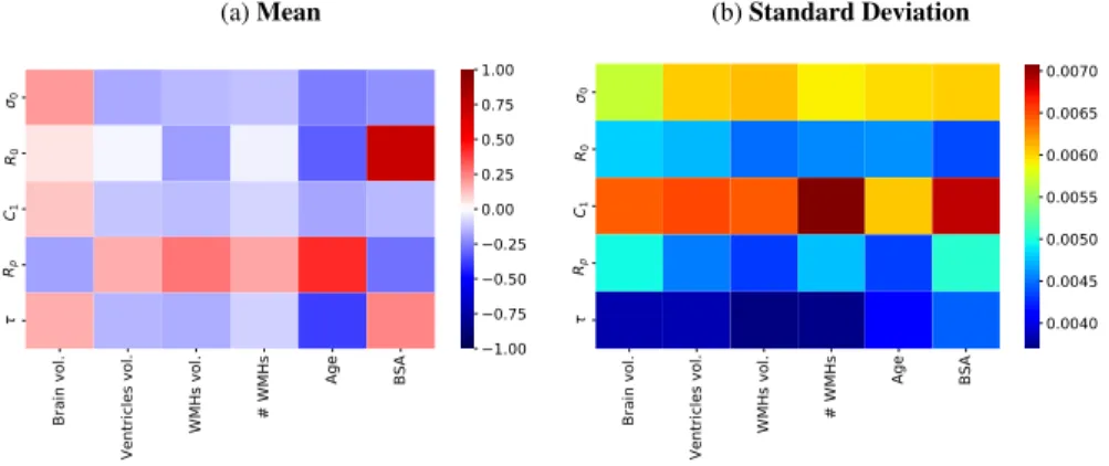
For each individual considered in this analysis we assessed the uncertainty in the parameter’s estimation using the covariance and the mean of the sampling distribution of the CMA-ES obtained at the last iteration of the IUP algorithm. In addition, we performed a sensitivity analysis to assess how this uncertainty propagates to the target features, and how it affects the relationship between the external features and the esti-mated parameters. The adopted procedure is as follows. For each subject we sampled 100 solutions, computed the fitting errors and assessed the correlations between the model parameters and the external features. The parameter’s uncertainty was quanti-fied by the standard deviation as a percentage of the mean value, while the fitting errors by the absolute error as a percentage of the target values. Table 2 summarises the ob-tained results. The median uncertainty in the parameters estimation is around 5% for every parameter and the highest upper quartile is close to 10%. Based on the estimated uncertainty of the fitting errors, we observe how solutions sampled around the selected hyper-plane in the parameter-space lead to reasonable solutions, the highest upper quar-tile for the mean error is below 7.5%, and below 5% for the standard deviation. Finally, Figure 7 shows the average correlations between the model parameters and the exter-nal features and their standard deviation. We can see how the average results match the ones presented in Figure 6b, while the standard deviation of the relationships is low, showing their stability.
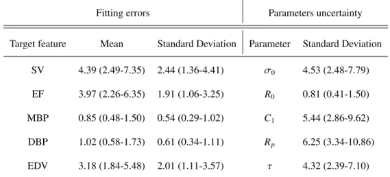
Table 2: We sampled 100 solutions for every subject by using their respective sampling distribution obtained by the CMA-ES optimisation at the last IUP iteration. Fitting errors quantified by means of the absolute error as a percentage of the target features. The target features are: stroke volume (SV), ejection fraction (EF), mean blood pressure (MBP), diastolic blood pressure (DBP) and end-diastolic volume (EDV). The uncertainty in the parameter’s estimation is assessed by means of the standard deviation as percentage of the mean value. The standard deviation and the mean were obtained from the sampling distribution of the CMA-ES. The sampled parameters are: contractility (σ0), ventricle radius (R0), stiffness (C1), peripheral resistance (Rp) and arterial compliance (τ). All the results are reported using the median and the interquartile range.
Fitting errors Parameters uncertainty
Target feature Mean Standard Deviation Parameter Standard Deviation
SV 4.39 (2.49-7.35) 2.44 (1.36-4.41) σ0 4.53 (2.48-7.79) EF 3.97 (2.26-6.35) 1.91 (1.06-3.25) R0 0.81 (0.41-1.50) MBP 0.85 (0.48-1.50) 0.54 (0.29-1.02) C1 5.44 (2.86-9.62) DBP 1.02 (0.58-1.73) 0.61 (0.34-1.11) Rp 6.25 (3.34-10.86) EDV 3.18 (1.84-5.48) 2.01 (1.11-3.57) τ 4.32 (2.39-7.10) 4.3. AF subgroup analysis
Considering the dataset obtained after the pre-processing steps described in Section 4.1 we obtained 59 subjects diagnosed with AF.
We analysed two aspects of this subgroup with respect to the population of healthy controls: 1) if there are significant differences in the correlations between the model parameters and the external features, and 2) if there are significant differences between the estimated model parameters between groups. Compatibly with the experiments shown in the previous section, we assessed these aspects through bootstraping of 100 training sets, composed by the 59 AF subjects and by a random control group matched with the AF sub-cohort without significant differences in age, sex and BSA, adding up to 118 subjects per training set. Each control group was sampled without replacement from the subset of subjects without any of the cardiovascular diseases listed in the appendix Table A.1 (n = 2892). Through this approach we can take into account the
(a) Mean
Brain vol.
Ventricles vol. WMHs vol.
# WMHs Age BSA 0 R0 C1 Rp 1.00 0.75 0.50 0.25 0.00 0.25 0.50 0.75 1.00 (b) Standard Deviation Brain vol.
Ventricles vol. WMHs vol.
# WMHs Age BSA 0 R0 C1 Rp 0.0040 0.0045 0.0050 0.0055 0.0060 0.0065 0.0070
Figure 7: We sampled 100 solutions for every subject by using their respective sampling distribution obtained by the CMA-ES optimisation at the last IUP iteration. a) Average correlations between model parameters and external features b) Standard deviation of the correlations. The average correlation matches the one presented in Figure 6b and the low variability seen in the standard deviation highlights the robustness of the estimated associations.
.
variability present in the whole personalisation process and in the healthy population. Furthermore, we assessed the significance for the differences between AF and controls, we created a sampling population composed of all the solutions obtained in the 100 training sets. Then, we estimated a null distribution of differences between randomly sampled groups with sample size corresponding to the ones of AF and controls groups respectively. This distribution allows us to quantify the distribution of the observed difference when the underlying difference between the groups is actually zero. Hence, we statistically assessed the significance of the observed difference between the AF and the control groups by comparison with the null distribution using a significance level of α= 0.05. The results presented in Table 3 show that there is a significant difference in their contractility, σ0, while other parameters such as the peripheral resistance, Rp,
or the left ventricle size, R0, are close to significance.
Moreover, the results from the 100 training sets allowed us to obtain an empirical distribution of the correlations between cardiac and external parameters. We assessed the differences between controls and AF groups using the Wilcoxon rank-sum test and considered them significant when one of the distributions was significantly greater or
Table 3: Results from the bootstrap analysis used to compare the AF and the control groups. The null-distribution for the difference was obtained by sampling with replacement 10,000 times two random groups with samples sizes matching those of of AF and control groups. We evaluated if the difference between the AF group and the control groups was significant according to a significance level of α= 0.05. The significant features are set in bold.
Parameter σ0 R0 C1 Rp τ
p-value 0.03 0.15 0.12 0.086 0.96
smaller than 0. All the tests were performed using a significance level of α = 0.05 adjusted using Bonferroni correction for 30 comparisons in total, accounting for the comparisons between the model parameters (5) and their association with the external features (6).
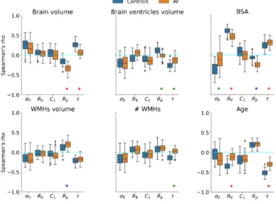
Figure 8: Comparison of the bootstrap distributions of the Spearman’s rank correlation coefficient obtained at regularisation (γ)= 1 between the personalised model parameters and the external features. Blue box-plots correspond to control groups and orange to AF subjects. ∗ denotes that the correlations are significantly different according to the Wilcoxon rank-sum test. In red both group correlations are significantly greater or smaller than 0 and there is change in the magnitude of the association. In blue the control group is not significantly greater or smaller than 0 and the AF group it is, so it represents a new association. In green we denote the opposite case, representing lost associations. All tests performed with a 5% significance level adjusted using Bonferroni correction.
60 80 100 120 140 160 Ventricle volume [ml] 0 25 50 75 100 125 150 Ve ntr icl e p ressu re [m mH g] AF Controls
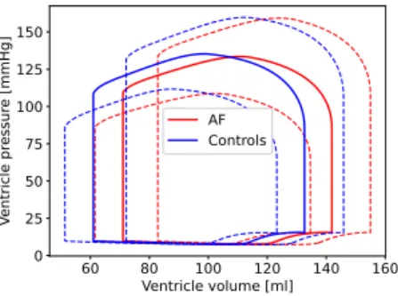
Figure 9: Pressure-volume (PV) loop comparison between AF (orange) and controls (blue). Solid lines (PV) represent the average loop and dashed lines the standard deviation.
Figure 8 reports the empirical distribution of correlations obtained from the bootstrap analysis performed in the AF subset. When distributions were statistically different we considered three different scenarios:
1. Change in magnitude (red): the control and AF distributions are significantly different from 0;
2. AF association (blue): only the AF group is significantly different from 0; 3. Control association (green): only the control group is significantly different from
0.
In the control group we can observe a pattern of associations similar to the one found in the whole-cohort analysis: brain volume is correlated with the contractility, σ0, and the arterial compliance, τ, while it is inversely associated to the peripheral
re-sistance, Rp. The inverse pattern is seen in the other brain indices (volume and number
of WMHs and ventricles volume) and age. On the other hand, the BSA is associated to the left ventricle radius, R0, and with lower contractility. In the AF group the
dif-ferences are mainly found in the associations involving the aortic compliance, τ, and the peripheral resistance, Rp. Compared to the control groups τ loses its association
with whole brain volume, ventricles volume, and with the number of WMHs. At the same time, the association between Rp and the total volume of WMHs becomes
sig-nificant, the one with brain volume gets stronger, while the relationship with brain ventricles volume is lost. Furthermore, the association between age and the size of the
left ventricle, R0, is lost and the one with the arterial compliance decreases in
magni-tude. Regarding BSA we observe how the association with the left ventricle size gets weaker, the one with the arterial compliance stronger, a new one with peripheral resis-tance appears and the one with the contractility, σ0, disappears. Figure 9 illustrates the
differences in the modeled PV loop between the average AF subject and the average control subject. In the AF subjects it can be appreciated an increased end-diastolic vol-ume and decreased end-systolic pressure volvol-ume relationship, indicating a decreased contractility, σ0, increased afterload, and a dilated ventricle.
The observed differences between AF and control subjects may be the result of several pathological processes. Recently some studies have proposed different mecha-nisms through which AF may promote cognitive decline and induce brain morphologi-cal changes (Dagres, 2018; Sepehri Shamloo et al., 2020). AF could lead to the forma-tion of small thrombus which in turn can result in small brain silent infarcts. In addiforma-tion, the increase in beat-to-beat variability may reduce the cardiac output (CO) leading to impaired brain perfusion. Impaired brain perfusion has been linked to increased WMHs and reduced cortical volumes (Alosco et al., 2013; Jefferson et al., 2009). The im-paired altered beat-to-beat variability may stress the autoregulatory mechanisms of the vascular system, inducing endothelial dysfunction and vascular remodelling processes (Xia et al., 2017). These processes commonly lead to the thickening of the arterioles and occlusion of capillaries which increase the peripheral resistance, Rp, and
subse-quently triggers the stiffening, τ, of large arteries (Da¸browska et al., 2020; Laurent and Boutouyrie, 2015). Indeed, a mechanistic approach already related AF to hypoperfuse events in the distal circulation (Scarsoglio et al., 2017). These processes may explain the changes in the associations between Rp, τ and the brain volumetric indices. The
in-creased peripheral resistance may result in an inin-creased afterload that leads to inin-creased atrial and ventricular filling pressures, which in turn can induce an enlargement of the chambers. This finding is supported by the known role of cardiac remodelling as a risk factor for AF (Seko et al., 2018; Lau et al., 2012), and could explain the changes in the associations of R0with age and BSA, as well as between σ0and BSA.
5. Discussion
To our knowledge this study presents the largest cohort of personalised subjects, 3445, being specifically focused on obtaining homogeneous solutions that enable to use the obtained model parameters in post-hoc analyses. The results presented in Sec-tion 4.2.2, in which we observe the lack of associaSec-tions between the target features and brain features, highlight the need of combining statistical learning with biophysical models to better understand the underlying physiology in medical data analysis. More-over, from the uncertainty analysis presented in Section 4.2.3 we can conclude that the solutions are stable and meaningful. However, due to the available data, the used car-diovascular features are mostly global features while other studies (M¨uller and Toro, 2014) suggest that brain indices such as WMHs are due to more localised vascular im-pairments. Hence, brain blood flow characterisation would be useful to estimate more relevant parameters, at least from the main cerebral vessels, which could be obtained from MR angiography images. Moreover, in our model there is no difference between ”upper” and ”lower” body circulation. Studies analysing the influence of AF in the brain, such as (Scarsoglio et al., 2017), have differentiated between those circulations. In the future the current biophysical model could be adapted to incorporate a bifurca-tion towards the upper body circulabifurca-tion. This would allow us to use pulse wave velocity (PWV) measurements at the carotid level to obtain patient-specific solutions in which we could estimate the brain blood flow perfusion. In turn, this would also allow to study the effect of the relative stiffening of the aorta compared to the carotid. Which, accord-ing to (Aghilinejad et al., 2020), is key to attenuate blood flow pulsatility in the brain microvasculature. Another issue to consider is that in our haemodynamic model wave propagation effects are neglected. If continuous blood pressure measurements were available at different locations we could replace the 0D haemodynamic component of our model by a 1D model while keeping a reasonable computational cost. Moreover, the use of continuous measures would allow to use other personalisation approaches such as Kalman filter (Pant et al., 2017) which can handle uncertainty in the param-eter’s estimation. Furthermore, currently the covariance matrix of our regularisation term is computed empirically. It would be interesting to explore its parametrisation by
means of a kernel or multiple kernels. For example, future work may focus on the study of the relative influence of the features by means of automatic relevance determination (ARD). Moreover, multiple kernels, one for the external features and another for the model parameters, could be used. However, these approaches would increase the com-plexity of the problem, since we would need to estimate the kernel hyper-parameters on top of the subject’s personalisation.
6. Conclusion
We presented a novel statistical learning framework to integrate prior physiolog-ical knowledge through biophysphysiolog-ical modelling. Its behaviour was exemplified with personalised lumped cardiovascular models on heart and brain data of 3445 subjects. This was achieved by constraining the available parameter-space during parameter op-timisation with external brain features in a regularisation term. The presence of the external features allowed to learn a more meaningful representation of the parameter-space enabling to study the interaction of brain features with cardiac model parameters and illustrating the potential use of the framework to estimate cardiac model param-eters using a limited amount of clinical information. Additionally, the presented ap-proach can be seen as a parameter selection apap-proach, as demonstrated in (Moll´ero et al., 2018), where they shown how the IUP algorithm can select linear subspaces in which non-observable parameters get close to constant values. The identification of non-observable parameters coupled with human modelling expertise can help in the selection of a reduced subset of observable cardiovascular parameters for personalisa-tion. Moreover, the use of this approach provides a generative model that allows to analyse the interaction between external features and non-observable parameters such as the aortic compliance, τ, or the peripheral resistance Rp, which we found to be
re-lated with brain-volumetric features. Using the same framework we assessed a clinical subgroup in which we found meaningful clinical relationships, linking AF with WMHs and heart remodelling. These results, along with the small associations between car-diac target features and brain indices, illustrate the potential of combining statistical learning with biophysical modelling. Future work will go towards incorporating brain
blood flow characterisation and the assessment of its spatial patterns.
Acknowledgements
This work has been supported by the Inria Sophia Antipolis - M´editerran´ee, ”NEF” computation cluster, and by the French government, through the 3IA Cˆote d’Azur In-vestments in the Future project managed by the National Research Agency (ANR) with the reference number ANR-19-P3IA-0002. This work was also supported by the Span-ish Ministry of Science, Innovation and Universities under the Retos I+D Programme (RTI2018-101193-B-I00) and the Maria de Maeztu Units of Excellence Programme (MDM-2015-0502). This research has been conducted using the UK Biobank Re-source undder Application Number 20576.
References
Aghilinejad, A., Amlani, F., King, K.S., Pahlevan, N.M., 2020. Dynamic Effects of Aortic Arch Stiffening on Pulsatile Energy Transmission to Cerebral Vasculature as A Determinant of Brain-Heart Coupling. Scientific Reports 10, 8784.
Akasheva, D.U., Plokhova, E.V., Tkacheva, O.N., Strazhesko, I.D., Dudinskaya, E.N., Kruglikova, A.S., Pykhtina, V.S., Brailova, N.V., Pokshubina, I.A., Sharashkina, N.V., Agaltsov, M.V., Skvortsov, D., Boytsov, S.A., 2015. Age-related left ventric-ular changes and their association with leukocyte telomere length in healthy people. PLoS ONE 10, 1–10.
Alfaro-Almagro, F., Jenkinson, M., Bangerter, N.K., Andersson, J.L., Griffanti, L., Douaud, G., Sotiropoulos, S.N., Jbabdi, S., Hernandez-Fernandez, M., Vallee, E., Vidaurre, D., Webster, M., McCarthy, P., Rorden, C., Daducci, A., Alexander, D.C., Zhang, H., Dragonu, I., Matthews, P.M., Miller, K.L., Smith, S.M., 2018. Image processing and quality control for the first 10,000 brain imaging datasets from uk biobank. NeuroImage 166, 400–424.
Alonso, A., Arenas de Larriva, A.P., 2016. Atrial Fibrillation, Cognitive Decline and Dementia. European Cardiology Review 11, 49.
Alosco, M.L., Brickman, A.M., Spitznagel, M.B., Garcia, S.L., Narkhede, A., Griffith, E.Y., Raz, N., Cohen, R., Sweet, L.H., Colbert, L.H., Josephson, R., Hughes, J., Rosneck, J., Gunstad, J., 2013. Cerebral Perfusion is Associated With White Matter Hyperintensities in Older Adults With Heart Failure. Congestive Heart Failure 19, E29–E34.
Azarpazhooh, M.R., Avan, A., Cipriano, L.E., Munoz, D.G., Sposato, L.A., Hachinski, V., 2018. Concomitant vascular and neurodegenerative pathologies double the risk of dementia. Alzheimer’s and Dementia 14(2), 148–156.
Bahrani, A.A., Powell, D.K., Yu, G., Johnson, E.S., Jicha, G.A., Smith, C.D., 2017. White Matter Hyperintensity Associations with Cerebral Blood Flow in Elderly Sub-jects Stratified by Cerebrovascular Risk. Journal of Stroke and Cerebrovascular Dis-eases 26, 779–786.
Banus, J., Lorenzi, M., Camara, O., Sermesant, M., 2019. Large Scale Cardiovascu-lar Model Personalisation for Mechanistic Analysis of Heart & Brain Interactions. Functional Imaging and Modelling of the Heart .
Benjamin, E.J., Virani, S.S., Callaway, C.W., Chang, A.R., Cheng, S., Chiuve, S.E., Cushman, M., Delling, F.N., Deo, R., de Ferranti, S.D., Ferguson, J.F., Fornage, M., Gillespie, C., Isasi, C.R., Jim´enez, M.C., Jordan, L.C., Judd, S.E., Lackland, D., Lichtman, J.H., Lisabeth, L., Liu, S., Longenecker, C.T., Lutsey, P.L., Matchar, D.B., Matsushita, K., Mussolino, M.E., Nasir, K., O’Flaherty, M., Palaniappan, L.P., Pandey, D.K., Reeves, M.J., Ritchey, M.D., Rodriguez, C.J., Roth, G.A., Rosamond, W.D., Sampson, U.K., Satou, G.M., Shah, S.H., Spartano, N.L., Tirschwell, D.L., Tsao, C.W., Voeks, J.H., Willey, J.Z., Wilkins, J.T., Wu, J.H., Alger, H.M., Wong, S.S., Muntner, P., 2018. Heart disease and stroke statistics—2018 update: A report from the american heart association. Circulation 137(12).
Caruel, M., Chabiniok, R., Moireau, P., Lecarpentier, Y., Chapelle, D., 2014. Dimen-sional reductions of a cardiac model for effective validation and calibration. Biome-chanics and Modeling in Mechanobiology 13, 897–914.
Chapelle, D., Le Tallec, P., Moireau, P., Sorine, M., 2012. Energy-preserving muscle tissue model: formulation and compatible discretizations. International Journal for Multiscale Computational Engineering 10(2), 189–211.
Chen, L.Y., Norby, F.L., Gottesman, R.F., Mosley, T.H., Soliman, E.Z., Agarwal, S.K., Loehr, L.R., Folsom, A.R., Coresh, J., Alonso, A., 2018. Association of atrial fibrillation with cognitive decline and dementia over 20 years: The ARIC-NCS (Atherosclerosis Risk in Communities Neurocognitive Study). Journal of the American Heart Association 7, 1–13.
Cox, S.R., Lyall, D.M., Ritchie, S.J., Bastin, M.E., Harris, M.A., Buchanan, C.R., Fawns-Ritchie, C., Barbu, M.C., De Nooij, L., Reus, L.M., Alloza, C., Shen, X., Neilson, E., Alderson, H.L., Hunter, S., Liewald, D.C., Whalley, H.C., McIntosh, A.M., Lawrie, S.M., Pell, J.P., Tucker-Drob, E.M., Wardlaw, J.M., Gale, C.R., Deary, I.J., 2019. Associations between vascular risk factors and brain MRI indices in UK Biobank. European Heart Journal 44, 1–11.
Da¸browska, E., Harazny, J.M., Miszkowska-Nag´orna, E., Stefa´nski, A., Graff, B., Kunicka, K., ´Swierblewska, E., Rojek, A., Szyndler, A., Wolf, J., Gruchała, M., Schmieder, R.E., Narkiewicz, K., 2020. Lumen narrowing and increased wall to lumen ratio of retinal microcirculation are valuable biomarkers of hypertension-mediated cardiac damage. Blood Pressure 29, 70–79.
Dagres, N., 2018. Expert consensus on arrhythmias and cognitive function: What is the best practice? Europace 20, 1399–1400.
Debette, S., Markus, H.S., 2010. The clinical importance of white matter hyperinten-sities on brain magnetic resonance imaging: systematic review and meta-analysis. Bmj 341, c3666–c3666.
Delingette, H., Billet, F., Wong, K.C., Sermesant, M., Rhode, K., Ginks, M., Rinaldi, C.A., Razavi, R., Ayache, N., 2012. Personalization of cardiac motion and con-tractility from images using variational data assimilation. IEEE Transactions on Biomedical Engineering 59, 20–24.
Doehner, W., Ural, D., Haeusler, K.G., ˇCelutkien˙e, J., Bestetti, R., Cavusoglu, Y., Pe˜na-Duque, M.A., Glavas, D., Iacoviello, M., Laufs, U., Alvear, R.M., Mbakwem, A., Piepoli, M.F., Rosen, S.D., Tsivgoulis, G., Vitale, C., Yilmaz, M.B., Anker, S.D., Filippatos, G., Seferovic, P., Coats, A.J., Ruschitzka, F., 2018. Heart and brain interaction in patients with heart failure: overview and proposal for a taxonomy. A position paper from the Study Group on Heart and Brain Interaction of the Heart Failure Association. European Journal of Heart Failure 20, 199–215.
Downey, J.M., Heusch, G., 2001. Sequence of Cardiac Activation and Ventricular Mechanics, in: Heart Physiology and Pathophysiology. Elsevier, pp. 3–18.
Friedman, J.I., Tang, C.Y., De Haas, H.J., Changchien, L., Goliasch, G., Dabas, P., Wang, V., Fayad, Z.A., Fuster, V., Narula, J., 2014. Brain imaging changes asso-ciated with risk factors for cardiovascular and cerebrovascular disease in asymp-tomatic patients. JACC: Cardiovascular Imaging 7, 1039–1053.
Hansen, N., 2016. The cma evolution strategy: A comparing review. Towards a New Evolutionary Computation 102, 75–102.
Hooghiemstra, A.M., Bertens, A.S., Leeuwis, A.E., Bron, E.E., Bots, M.L., Brunner-La Rocca, H.P., De Craen, A.J., Van Der Geest, R.J., Greving, J.P., Kappelle, L.J., Niessen, W.J., Van Oostenbrugge, R.J., Van Osch, M.J., De Roos, A., Van Rossum, A.C., Biessels, G.J., Van Buchem, M.A., Daemen, M.J., Van Der Flier, W.M., 2017. The Missing Link in the Pathophysiology of Vascular Cognitive Impairment: Design of the Heart-Brain Study. Cerebrovascular Diseases Extra 7, 140–152.
Iadecola, C., 2013. The pathology of vascular dementia. Neuron 80, 844–866. Jani, B., Rajkumar, C., 2006. Ageing and vascular ageing. Postgraduate Medical
Journal 82, 357–362.
Jefferson, A.L., Tate, D.F., Poppas, A., Brickman, A.M., Paul, R.H., Gunstad, J., Co-hen, R.A., 2009. Lower Cardiac Output Is Associated with Greater White Matter Hyperintensities in Older Adults with Cardiovascular Disease. J Am Geriatr Soc 55, 1044–1048.
Jegier, W., Sekelj, P., Auld, P.A., Simpson, R., McGregor, M., 1963. the Relation Between Cardiac Output and Body Size. British heart journal 25, 425–430.
Khalil, A.S., Bouma, B.E., Kaazempur Mofrad, M.R., 2006. A combined FEM/genetic algorithm for vascular soft tissue elasticity estimation. Cardiovascular Engineering 6, 93–102.
Lau, Y.F., Yiu, K.H., Siu, C.W., Tse, H.F., 2012. Hypertension and atrial fibrillation: Epidemiology, pathophysiology and therapeutic implications. Journal of Human Hypertension 26, 563–569.
Laurent, S., Boutouyrie, P., 2015. The Structural Factor of Hypertension: Large and Small Artery Alterations. Circulation Research 116, 1007–1021.
Marchesseau, S., Delingette, H., Sermesant, M., Ayache, N., 2013. Fast parameter calibration of a cardiac electromechanical model from medical images based on the unscented transform. Biomechanics and Modeling in Mechanobiology 12, 815–831. Modir, R., Gardener, H., Wright, C.B., 2012. Stroke blood pressure and white matter hyperintensity volume — a review of the relationship and implications for stroke prediction and prevention. US Neurology 8(1), 33–36.
Moll´ero, R., Pennec, X., Delingette, H., Ayache, N., Sermesant, M., 2018. Population-based priors in cardiac model personalisation for consistent parameter estimation in heterogeneous databases. International Journal for Numerical Methods in Biomedi-cal Engineering. .
Moll´ero, R., Pennec, X., Delingette, H., Garny, A., Ayache, N., Sermesant, M., 2017. Multifidelity-cma: a multifidelity approach for efficient personalisation of 3d cardiac electromechanical models. Biomechanics & Modeling in Mechanobiology 17(1), 285–300.
Moroni, F., Ammirati, E., Rocca, M.A., Filippi, M., Magnoni, M., Camici, P.G., 2018. Cardiovascular disease and brain health: Focus on white matter hyperintensities. IJC Heart and Vasculature 19, 63–69.
Mosteller, R., 1987. Simplified calculation of body-surface area. The new england journal of medicine 17, 1098.
Muiesan, M.L., Salvetti, M., Paini, A., Agabiti-Rosei, C., Bertacchini, F., Maruelli, G., Colonetti, E., 2014. Central blood pressure assessment using 24-hour brachial pulse wave analysis. Journal of Vascular Diagnostics , 141.
M¨uller, L.O., Toro, E.F., 2014. Enhanced global mathematical model for studying cerebral venous blood flow. Journal of Biomechanics 47(13), 3361–3372.
Neumann, D., Mansi, T., Itu, L., Georgescu, B., Kayvanpour, E., Sedaghat-Hamedani, F., Amr, A., Haas, J., Katus, H., Meder, B., Steidl, S., Hornegger, J., Comaniciu, D., 2016. A self-taught artificial agent for multi-physics computational model personal-ization. Medical Image Analysis 34, 52–64.
Ois, A., Gomis, M., Cuadrado-Godia, E., Jim´enez-Conde, J., Rodr´ıguez-Campello, A., Bruguera, J., Molina, L., Comin, J., Roquer, J., 2008. Heart failure in acute ischemic stroke. Journal of Neurology 255(3), 385–389.
Pant, S., Corsini, C., Baker, C., Hsia, T.Y., Pennati, G., Vignon-Clementel, I.E., 2017. Inverse problems in reduced order models of cardiovascular haemodynamics: As-pects of data assimilation and heart rate variability. Journal of the Royal Society Interface 14.
Pant, S., Fabr`eges, B., Gerbeau, J.F., Vignon-Clementel, I.E., 2014. A methodolog-ical paradigm for patient-specific multi-scale CFD simulations: from clinmethodolog-ical mea-surements to parameter estimates for individual analysis. International Journal for Numerical Methods in Biomedical Engineering 30, 1614–1648.
Ribaldi, F., Jovicich, J., Ferrari, C., Bosch, B., Bartr´es-Faz, D., M¨uller, B.W., Wiltfang, J., Fiedler, U., Montalti, M., Roccatagliata, L., Picco, A., Nobili, F., Blin, O., Bom-bois, S., Lopes, R., Bordet, R., Sein, J., Ranjeva, J.P., Didic, M., Gros-Dagnac, H., Payoux, P., Alessandrini, F., Beltramello, A., Bargallo, N., Ferretti, A., Caulo, M., Aiello, M., Cavaliere, C., Soricelli, A., Parnetti, L., Tarducci, R., Floridi, P., Tso-laki, M., Constantinides, M., Drevelegas, A., Rossini, P., Marra, C., Schonknecht,
P., Hensch, T., Hoffmann, K.T., Kuijer, J., Visser, P.J., Barkhof, F., Frisoni, G.B., Marizzoni, M., 2018. Ic-P-126: Volumetric Accuracy of a Fully Automatic Tool for White Matter Hyperintensities (Wmhs) Segmentation. Alzheimer’s & Dementia 14, P105–P106.
Scarsoglio, S., Saglietto, A., Anselmino, M., Gaita, F., Ridolfi, L., 2017. Alteration of cerebrovascular haemodynamic patterns due to atrial fibrillation: An in silico investigation. Journal of the Royal Society Interface 14.
Schmidt, P., 2017. Bayesian inference for structured additive regression models forlarge-scale problems with applications to medical imaging. PhD thesis, Ludwig-Maximilians-Universit¨at M¨unchen .
Seko, Y., Kato, T., Haruna, T., Izumi, T., Miyamoto, S., Nakane, E., Inoko, M., 2018. Association between atrial fibrillation, atrial enlargement, and left ventricular geo-metric remodeling. Scientific Reports 8(1), 1–8.
Sepehri Shamloo, A., Dagres, N., M¨ussigbrodt, A., Stauber, A., Kircher, S., Richter, S., Dinov, B., Bertagnolli, L., Husser-Bollmann, D., Bollmann, A., Hindricks, G., Arya, A., 2020. Atrial Fibrillation and Cognitive Impairment: New Insights and Future Directions. Heart Lung and Circulation 29, 69–85.
Sudlow, C., Gallacher, J., Allen, N., Beral, V., Burton, P., Danesh, J., Downey, P., Elliott, P., Green, J., Landray, M., Liu, B., Matthews, P., Ong, G., Pell, J., Silman, A., Young, A., Sprosen, T., Peakman, T., Collins, R., 2015. Ukbiobank an open access resource for identifying the causes of a wide range of complex diseases of middle and old age. PLoS Med. 12, 1–10.
Veldsman, M., Tai, X.Y., Nichols, T., Smith, S., Peixoto, J., Manohar, S., Husain, M., 2020. Cerebrovascular risk factors impact frontoparietal network integrity and executive function in healthy ageing. Nature Communications 11, 1–10.
Wardlaw, J.M., Vald´es Hern´andez, M.C., Mu˜noz-Maniega, S., 2015. What are white matter hyperintensities made of? relevance to vascular cognitive impairment. Jour-nal of the American Heart Association 4(6).
Xia, Y., Liu, X., Wu, D., Xiong, H., Ren, L., Xu, L., Wu, W., Zhang, H., 2017. Influence of beat-to-beat blood pressure variability on vascular elasticity in hypertensive pop-ulation. Scientific Reports 7, 8394. URL: http://www.nature.com/articles/ s41598-017-08640-4, doi:10.1038/s41598-017-08640-4.
Zhang, Y., Brady, M., Smith, S., 2001. Segmentation of brain MR images through a hidden Markov random field model and the expectation-maximization algorithm. IEEE Transactions on Medical Imaging 20, 45–57.
Appendix A. UK Biobank data codes
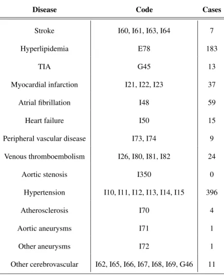
Table A.1: List of considered cardiovascular diseases and their correspondent ICD10 codes
Disease Code Cases
Stroke I60, I61, I63, I64 7
Hyperlipidemia E78 183
TIA G45 13
Myocardial infarction I21, I22, I23 37
Atrial fibrillation I48 59
Heart failure I50 15
Peripheral vascular disease I73, I74 9
Venous thromboembolism I26, I80, I81, I82 24
Aortic stenosis I350 0
Hypertension I10, I11, I12, I13, I14, I15 396
Atherosclerosis I70 4
Aortic aneurysms I71 1
Other aneurysms I72 1
Other cerebrovascular I62, I65, I66, I67, I68, I69, G46 11
Table A.2: UK Biobank data-fields corresponding to the used data. In all the cases the data timepoint was 2.0, corresponding to the first imaging visit.
Data Code
Sex 31
Age attended centre 21003
Standing Height 50
Weight 21002
DBP automated 4079
SBP automated 4080
Left ventricle SV 22423
Left ventricle EDV 22421
Left ventricle ESV 22422
Left ventricle EF 22420
Volume WM normalized 25007
Volume GM normalized 25005
Volume Ventricles normalized 25003
Table B.3: Default values of the cardiovascular model’s parameters. The varying parameters are set in bold.
Left heart Value Right heart Value Concept
Heart period[s] 0.8 Heart period[s] 0.8 Heart period
α [a.u] 1.5 α [a.u] 1.5 Cross-bridge destruction upon rapid length changes
w[a.u] 1 w[a.u] 1 Length-dependent relaxation
n0[a.u] 1 n0[a.u] 1 Length-dependent fraction of myosin heads
k0[Pa] 1 · 105 k
0[Pa] 1 · 105 Sarcomere stiffness
σ0[Pa] 6.4 · 104 σ0[Pa] 6.4 · 104 Maximum sarcomere active stress (Contractility)
kAT P[s−1] 30 kAT P[s−1] 30 Speed of sarcomere force build-up (ATP rate)
krs[s−1] 30 krs[s−1] 30 Speed of sarcomere force decrease (Relaxation rate)
APD[s] 0.30 APD[s] 0.30 Action potential duration
AV delay[s] 0.12 AV delay[s] 0.12 Atrioventricular delay
QRS duration[s] 0.085 QRS duration[s] 0.085 QRS duration
R0[m] 0.028 R0[m] 0.028 Ventricular resting radius
d0[m] 0.014 d0[m] 0.007 Ventricular wall thickness
ρ [kg.m−3] 1070 ρ [kg.m−3] 1070 Myocardial mass density
Es[Pa] 3 · 107 Es[Pa] 3 · 107 Ventricular elastance
µ [Pa.s] 70 µ [Pa.s] 70 Active viscous damping
c1[Pa] 1000 c1[Pa] 1000 Mooney-Rivlin material parameter (Stiffness)
c2[Pa] 1000 c2[Pa] 1000 Mooney-Rivlin material parameter (Stiffness)
η [Pa.s−1] 100 η [Pa.s−1] 100 Global damping
Pat t1[s] 0.005 Pat t1[s] 0.005 Start of atrial systole
Pat t2[s] 0.1 Pat t2[s] 0.1 Time peak of atrial systole
kat[m3.s−1.Pa−1] 9 · 10−6 kat[m3.s−1.Pa−1] 9 · 10−6 Atrioventricular valve resistance
kar[m3.s−1.Pa−1] 1.3 · 10−5 kar[m3.s−1.Pa−1] 1.3 · 10−5 Arterial valve resistance
kiso[m3.s−1.Pa−1] 1 · 10−37 kiso[m3.s−1.Pa−1] 1 · 10−37 Atrioventricular valve leakage
τ [s] 0.8 τ [s] 0.8 Windkessel time constant (τ= RpCar), where, Caris the aortic compliance
Rp[Pa.m−3.s] 2.5 · 107 Rp[Pa.m−3.s] 1 · 107 Peripheral resistance
Zc[Pa.m−3.s] 5 · 106 Z
c[Pa.m−3.s] 5 · 105 Proximal resistance
dt[s] 1 · 10−5 dt[s] 1 · 10−5 Time-step
V0at[m3] 0 V0at[m3] 0 Initial atrial volume
EatU pper[Pa.m−3] 2.2 · 107 EatU pper[Pa.m−3] 2.2 · 107 Maximum atrial elastance
EatLower[Pa.m−3] 1 · 107 EatLower[Pa.m−3] 1 · 107 Minimial atrial elastance
Pat t3[s] 0.2 Pat t3[s] 0.2 End of atrial systole
Systemic veins Value Pulmonary veins Value Concept
Rven[Pa.m−3.s] 2.5 · 107 Rven[Pa.m−3.s] 5 · 106 Venous resistance
Cven[m3.Pa−1] 5 · 10−6 Cven[m3.Pa−1] 5 · 10−5 Venous compliance
Algorithm 2 Scaled CMA optimization pseudo-code. 1: Inputs: 2: T ol µ∗,Σ∗, C s, ms C MAoptions 3: Returns: 4: θ∗, Cs, ms 5: Initialize: 6: Sbest s ← in f
7: while j< CMAiterationsdo 8: if msis null then
9: Initialize subjects’s covariance (Cs) and mean (ms) with parameter’s default
values
10: end if
11: ˆxs← sample from CMA (C MAoptions)
12: θs= ˆxs∗ C
1/2
s + ms
Ss= S (θs, ˆOs, µ∗, Σ∗, T ol) Evaluate solutions 13: if min(Ss) < Sbests then
14: Sbest s = min(Ss) θbest s ←θs θ∗ s = arg minSs(θs) 15: end if 16: if Sbests < Cththen 17: break 18: end if 19: end while 20: ms← mean of θbests