Guided wave propagation and scattering in pipeworks comprising elbows: Theoretical and experimental results

(1)

HAL Id: cea-01836058

https://hal-cea.archives-ouvertes.fr/cea-01836058

Submitted on 11 Jan 2019

HAL is a multi-disciplinary open access archive for the deposit and dissemination of sci-entific research documents, whether they are pub-lished or not. The documents may come from teaching and research institutions in France or abroad, or from public or private research centers.

L’archive ouverte pluridisciplinaire HAL, est destinée au dépôt et à la diffusion de documents scientifiques de niveau recherche, publiés ou non, émanant des établissements d’enseignement et de recherche français ou étrangers, des laboratoires publics ou privés.

Guided wave propagation and scattering in pipeworks

comprising elbows: Theoretical and experimental results

B Bakkali, A. Lhémery, B Baronian, B. Chapuis

To cite this version:

B Bakkali, A. Lhémery, B Baronian, B. Chapuis. Guided wave propagation and scattering in pipeworks comprising elbows: Theoretical and experimental results. Journal of Physics: Conference Series, IOP Publishing, 2015, 581, pp.012011. �10.1088/1742-6596/581/1/012011�. �cea-01836058�

(2)

Guided wave propagation and scattering in pipeworks

comprising elbows: Theoretical and experimental results

M El Bakkali1_{, A Lhémery}1_{, V Baronian}1_{and B Chapuis}1

CEA, LIST – F- 91191 Gif-sur-Yvette, France

E-mail : alain.lhemery@cea.fr

Abstract. Elastic guided waves (GW) are used to inspect pipeworks in various industries. Modelling tools for simulating GW inspection are necessary to understand complex scattering phenomena occurring at specific features (welds, elbows, junctions…). In pipeworks, straight pipes coexist with elbows. GW propagation in the former cases is well-known, but is less documented in the latter. Their scattering at junction of straight and curved pipes constitutes a complex phenomenon. When a curved part is joined to two straight parts, these phenomena couple and give rise to even more complex wave structures. In a previous work, the Semi-Analytic Finite Element method extended to curvilinear coordinates was used to handle GW propagation in elbows, combined with a mode matching method to predict their scattering at the junction with a straight pipe. Here, a pipework comprising an arbitrary number of elbows of finite length and of different curvature linking straight pipes is considered. A modal scattering matrix is built by cascading local scattering and propagation matrices. The overall formulation only requires meshing the pipe section to compute both the modal solutions and the integrals resulting from the mode-matching method for computing local scattering matrices. Numerical predictions using this approach are studied and compared to experiments.

1. Introduction

Thanks to their ability to propagate over long distance without attenuation, elastic guided waves (GW) are used in efficient non-destructive testing (NDT) operations for the in-service inspection of industrial pipeworks. However, because of the multi-modal and dispersive properties of GW, scattering phenomena involved when GW interact with specific features in the pipework are complex. Tools for simulating non-destructive examinations are thus useful to understand measured signals and to design or improve testing configurations.

In a straight pipe, GW propagation is well known: efficient computational methods are used to predict them such as the Semi-Analytic Finite Element method (SAFE) or the Finite Element (FE) method. Conversely, the GW propagation in curved guides, which are common in industrial plants, is less documented [1-2] and more difficult to model. In pipeworks, curved guides coexist with straight ones; hence, the scattering of GW at their junction is an important problem.

The aim of the present work is to study numerically and experimentally the GW propagation in a pipe elbow linked to straight parts using a modal approach in order to supplement capabilities of CIVA platform [3]. For this, a numerical model able to deal with curved guides is developed. This model is based on an extension of the SAFE method, commonly used to simulate the GW propagation in straight guides. Once the modal solution for GW in an elbow is obtained, the scattering at the junction between a straight and a curved guide is investigated. A numerical model based on the mode matching method is used to predict the modal decomposition of an incident mode scattered at such junction. Then, a global scattering matrix is built, accounting for the scattering at several junctions and for the guided propagation in between. An example of parametric study is given to illustrate the model capabilities. Experiments on an elbow of typical industrial characteristics are made for validation.

Mode conversions arising by the scattering of guided waves at the junction between a curved guide and a straight guide have been investigated. Finally, numerical results are compared to experimental studies in order to illustrate the capabilities of this model.

13th Anglo-French Physical Acoustics Conference (AFPAC2014) IOP Publishing Journal of Physics: Conference Series 581 (2015) 012011 doi:10.1088/1742-6596/581/1/012011

(3)

2. Semi-analytical model for guided waves propagations in pipe works comprising elbows In this section the overall modelling approach is summarized. Readers interested in its detailed derivation are referred to Ref. 4.

2.1. SAFE model in curvilinear coordinate system

The SAFE method is a numerical model used to describe the GW propagation in a waveguide in terms of a modal decomposition of elastodynamic fields. The GW modal basis is the solution of the wave equation in an elastic guide assumed to be homogeneous and to have free boundaries. The equation of motion writes: . , on 0 ) ( , in 0 ) ( l 2           n u u u div     (1) where u is the displacement, ρ the mass density, ω the pulsation,  the guide section and 1 its

guiding surface. At a given frequency, the semi-analytical finite element (SAFE) method allows solving Eq. (1) in the cross section of the guide by a finite element computation, the dependency upon the guiding axis being handled analytically, assuming invariant cross section and material properties along the propagation axis.

Contrary to the case of a straight guide, the Cartesian basis is inadequate to satisfy this condition for a curved guide. Hence, the SAFE formulation has to be written in a curvilinear coordinates system, also known as the Serret-Frenet basis. Figure 1 illustrates the new coordinate system for a curved waveguide (a ring torus):

Figure 1 : Schematic of a curved guide with local curvilinear coordinates (N, B, T) system associated to curved guide.

The three axes of this local basis are obtained from the expression of the position vector defining the centerline of the curved guide. The metric tensor of this covariant basis, necessary to define the elementary volume, is given by:

            2 ) 1 ( 0 0 0 1 0 0 0 1 x  g (2)

where = 1 / Rc is the curvature and x the coordinate in the normal direction N of each node of the

guide section.

(4)

To integrate the variational formulation in a curvilinear basis, an elementary volume corresponding to the coordinate differentials (dx, dy, ds) must be expressed in this basis [5]. This volume dV is defined using g1, g2 and g3 the axes of the non-orthonormal covariant basis associated to the curvilinear basis as follows: T g B g N g g ) g .(g g 3 2 1 3 2 1 ) 1 ( and , with . ) det( x dxdyds dxdyds dV         (3)

Assuming a time harmonic e(-jt)_{dependency and similarly to the classical case of a straight guide}

in the Cartesian coordinates system, the 3D variational formulation must first be written in the non-orthonormal covariant basis. Then, using the relation between the covariant and the curvilinear basis, each term of the variational formulation can be expressed in the curvilinear (N, B, T) basis. The final expression is given by:

2 ( ) ( ) det det 0, with ( , , ) ( , ) i ks t and ( , , ) ( , ) i ks t , dxdyds dxdyds x y s x y e  x y s x y e                



T



T

cur cov cur cur

cur cur cur cur

ε Cσ (g) u u (g)

u u u u (4)

with

ε

cur

, σ

curand

u

cur

,

are the strain, stress and displacement fields in curvilinear coordinates.

Once the variational formulation (4) has been written in the curvilinear basis, the above-mentioned condition is satisfied and the s dependency of the displacement is restricted to the argument of the exponential of propagation, e(jks)_{, which can be factorized in all elastodynamic field components. From}

this, the 3D variational formulation can be turned into a semi-analytical variational formulation by restricting the volume integration to a surface integration over the guide cross section. Finally, the numerical expression is written as:

0 2 2 _ _   K K )U M U (K e e 3 e 2 e 1 j   , (5)

where U is the displacement vector and β the wavenumber. e 1,2,3) i(i

K  and Me are the elementary

stiffness and mass matrices in the (N, B, T) basis, respectively, expressed as:

det( ) , det( ) , det( ) , det( ) . e e e e S S S S dxdy dxdy dxdy



dxdy    



e eT T e e eT T e 1 xy xy 2 xy s e eT T e e eT e 3 xy s K N L CL N g K N L CL N g K N L CL N g M N N g (6)

Ne_{is the finite element interpolation matrix and} T xy

L , T s

L are the elementary matrices introducing the curvature effect defined by Treyssède and Laguerre [6]. For a zero-curvature, these matrices exactly equal the well-established matrices for a straight waveguide.

At a given frequency and both in a straight and in a curved guide, the solution of the quadratic eigenvalue system of Eq. (5) allows us to compute the modal solution by calculating the eigenvalues and the eigenvectors, which correspond respectively to the wavenumbers and the vectors of particle displacement of every mode (propagative, evanescent and inhomogeneous).

2.2. The mode matching model at the junction of two guides

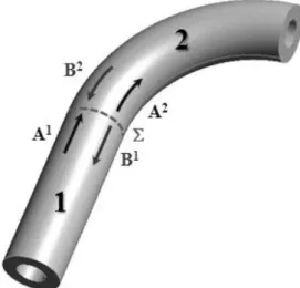
In a pipework comprising curved parts, pipe elbows are generally joined to straight pipes. When guided waves propagate, scattering phenomena arise at such junctions. Here, we aim at computing the corresponding scattering matrix for predicting the reflection and transmission phenomena occurring at the junction as illustrated by figure 2.

(5)

Figure 2 : Incoming and outgoing families of modes at the junction between the straight and the curved guides.

Assuming the completeness of the calculated eigenmodes obtained using the appropriate SAFE model, elastodynamic fields in the straight and in the curved parts are expressed as modal series of guided modes traveling in opposite directions as shown by Fig. 2 and in the following equation,

z jβ n n n n z jβ n n n n e n B e n A   _    



                    Y X Y X Y X (7) where X = (σxy, σyz, uz)T and Y= (ux, uy, -σzz)T are the hybrid vectors introduced by [7] and coupling

displacement and stress components of the elastodynamic field, Xn and Yn are the hybrid vectors of

each eigenmode obtained using SAFE with  __ 

n n X X ,  _  n n Y Y ,  __  n n



, An and Bn represent

the amplitudes of right going and the left going modes in each guide.

At the junction, the two elastodynamic fields associated to the different parts of the pipework and expressed by Eq. (7) must satisfy the continuity condition.In the present case, the elastodynamic fields are those associated to the straight (superscript 1) and the curved (superscript 2) parts of the pipework. Then, the continuity is written as:

s jβ n n n n s jβ n n n n z jβ n n n n z jβ n n n n 0 n n n n B e A e B e e A z s at z 2 2 2 2 2 2 2 2 2 2 2 1 1 1 1 1 1 1 1 1 1 1 1 2 2 2 2 2 2 1 1 1 1 1 1 2 2 1 1    



_                                                 Y X Y X Y X Y X Y X Y X (8)

Following Feng et al. [8] and using the biorthogonality relation (Fraser’s relation), the mode matching method expresses the relation between the amplitudes of the outgoing and the incoming modes by projecting Eq. (8) on the modal basis calculated by SAFE. Finally, one gets the following expression for the scattering matrix S at the junction:

1 2 2 1 1 1 2 2 1 2 2 1 1 2 2 1 1 2 1 1 2 1 2 2 1 1 2 2 1 2 2 1 1 2 , T T N N , , , , T T , , , , N N                              _{ } _ _{ } _ _    _{ }  1 B A S A B [0] J J R T 2J J J S T R J J 2J J J [0] (9) 13th Anglo-French Physical Acoustics Conference (AFPAC2014) IOP Publishing Journal of Physics: Conference Series 581 (2015) 012011 doi:10.1088/1742-6596/581/1/012011

(6)

whereR₁₂, T12 (R21,T21) are the reflection and transmission matrices for incident modes in the

straight part (respectively, in the curved part). Ni (i = 1, 2) denote the numbers of modes considered for

applying the mode matching in each part of the guide. All the propagative modes in both parts are taken into account together with a number of evanescent modes for reducing numerical errors. Jiand

Ji,j are the projection matrices of the elastodynamic fields calculated with the bi-orthogonality relation.

Their elementary components for the n-th mode in guide 1 onto the m-th mode in guide 1 [Eq. (10a)] or in guide 2 [Eq. (10b)] are defined as:

, ( , ) i i i( , ) ( , ) det( )i i i i, i n m n m i n m n s m J n m x y x y dxdy   (X Y )

_

X Y g  X M Y (10a) . ) det( ) , ( ) , ( ) , ( j ,j in nj in nj in sj nj i n m x y x y dxdy J (X Y )



X Y g XM Y  i)((10b) i s

M (i =1, 2) are the finite element projection matrices associated with the straight and the curved guides. These matrices are obtained from the global mass matrices calculated by the SAFE models and differ in each guide.

2.3.

Expression of the global scattering matrix

As shown previously, the mode matching method computes the scattering matrix of the junction by predicting the local phenomena linking two different elastodynamic fields computed by SAFE. However, pipeworks generally comprise a succession of junctions (similar or dissimilar). At each junction, various GW scattering phenomena occur which can be translated mathematically in the form of a specific modal scattering matrix. It is of course interesting to develop a way of predicting the overall GW propagation through a series of scatterers, similarly translated mathematically as a global matrix. Such an overall formulation of general applicability has been recently developed by two of the present authors [9]. In this formulation, a modal scattering matrix is obtained by cascading local scattering matrices (junctions, defects, etc.) and modal matrices accounting for the GW propagation back and forth in between.

In this section, this theory initially derived for straight guiding portions is adapted to deal with locally curved parts, our aim being to deal with the GW scattering by an elbow joined to two straight tubes.

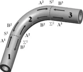
The global scattering matrix must deal with the multiple reflections between the two junctions and associated transmissions by linking the amplitudes of incoming modes to those of outgoing modes of the two straight parts of the pipework as illustrated in Fig 3:

Figure 3 : Incoming and outgoing families of modes in a straight-curved-straight guide.

(7)

According to [9], the global scattering matrix is a combination of the local scattering matrices S1

and S2 at the two junctions and the propagation matrix of the modes in the elbow. This latter is easily

adapted here to the case of a curved guide by using the curvilinear length sc =Rc θc of the centreline of

the elbow; it writes:

2 elbow 1 n c i s n N e    P diag( ) (11)

and the global scattering matrix is given by:

                    3 13 31 1 G G G G G 3 1 G 3 1 withS _TR T_R B A S A B (12)

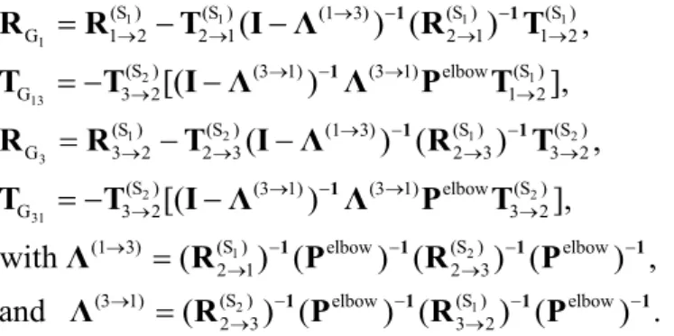
From this expression of , it is easy to extract the modal decomposition of incident modes in either one of the straight parts as reflected or transmitted modal components in the same part or in the other part. Reflection and transmission sub-matrices in Eq. (12) are given by [9]:

1 1 1 1 1 2 1 13 1 2 1 2 3 2 31 (S ) (S ) (1 3) (S ) (S ) G 1 2 2 1 2 1 1 2 (S ) (3 1) (3 1) elbow (S ) G 3 2 1 2 (S ) (S ) (1 3) (S ) (S ) G 3 2 2 3 2 3 3 2 (S ) (3 1) (3 1) elbow G 3 2 3 2 ( ) ( ) , [( ) ], ( ) ( ) , [( )                                     1 1 1 1 1 1 R R T I Λ R T T T I Λ Λ P T R R T I Λ R T T T I Λ Λ P T 2 1 2 2 1 (S ) (S ) (S ) (1 3) elbow elbow 2 1 2 3 (S ) (S ) (3 1) elbow elbow 2 3 3 2 ], with ( ) ( ) ( ) ( ) , and ( ) ( ) ( ) ( ) .                 1 1 1 1 1 1 1 1 Λ R P R P Λ R P R P (13)

The notations and have an obvious meaning of reflection and transmission matrices related to the two junctions. The same approach is straightforwardly generalized for computing the global scattering matrix of a pipework comprising several elbows with different curvatures by cascading the appropriate scattering and propagation matrices.

3. An illustrative example of GW scattering by an elbow

Consider an incident T(0,1) mode (commonly used in NDT operations in pipeworks) in a straight-curved-straight guide with an elbow of 120° as shown in Figure 4.

Figure 4 : Modal decomposition of an incident T(0,1) mode propagating in an elbow.

(8)

The energy ratios of an incident T(0,1) among transmitted modes at a single straight/curved junction and in an entire elbow as a function of the frequency are shown on Figure 5 (a) and (b):

Figure 5(b) : Transmitted energy for an incident T(0,1) mode vs. frequency.

Three frequency bands can be distinguished. The first one ([0-87] kHz) is characterized by a weak transmission and weak mode conversions considering the entire elbow despite the fact that the incident mode is highly transmitted at the first junction of the guide, except around the frequency for which the value of the T(0,1) wavelength equals the length of elbow centerline. In the second band ([87-100] kHz), the transmission still very high at the first junction and the entire elbow becomes almost transparent (high transmission ratio) with a very weak mode conversion; such a frequency range could be exploited for inspecting long pipeworks comprising several similar elbows. Finally, in the third band ([100-150] kHz), increasing mode conversion occurs at the single junction as well as in the entire elbow, notably into a high amplitude transmitted flexural mode F(1,2), though energy transmitted as a T(0,1) mode is still important at low frequencies of this band but decreases as the frequency increases. This result clearly shows that the chosen working frequency range is an important criterion which directly influences the guided waves behaviour when GW propagation in pipeworks comprising elbows is considered. These curves can be very useful for industrial inspections; in practice, it can help

Figure 5(a) : Transmitted energy for an incident T(0,1) mode at a single junction between a straight and a curved guide

(9)

to identify the appropriate frequency range to get the most efficient transmission or reflection phenomena and to anticipate modes conversions at each junction of the considered pipeworks and multiple reflections between junctions.

4. Experimental investigation of guided wave propagation in an industrial elbow 4.1. Experimental set-up

An experimental study was performed in collaboration with the Cetim (Technical Center for the mechanical industry) in order to investigate the effect of curvature on the guided waves propagation in industrial pipeworks comprising elbows. The experimental model consists in a 6 inches and a 7.1mm thickness steel pipe with an elbow of 30° and 437mm bend radius joined to two straight parts as shown in Figure 6:

Figure 6: The industrial pipework used for the experimental study.

Figure 7 illustrate the different features of our experimental model and their position:

Figure 7: Schematic view of the experimental model.

The data acquisition device consists of the MsS System [10] produced by Guided Wave Analysis LLC (GWA) and a point-like piezoelectric (Teletest) shear wave receiver produced by Plant integrity LTD (Pi) [12]. The MsS system is a magnetostrictive device used to generate and receive low-frequency (20 kHz to 250 kHz) guided waves (T(0,1) and L(0,2)) for NDT operations.

In our case, the system is exclusively used as a guided waves generator in a pulse/echo configuration (The emitter and the receiver are combined in a unique MsS patch) to generate the first torsional mode T(0,1) which is the only non-dispersive propagative mode (see Figure 8(a)).

The point-like Teletest sensor (see figure 8(b)) is an instrumented shear wave sensor coupled to the pipe with a shear gel and used as receiver. The experimental set-up is also composed of a digital oscilloscope to record filtered and amplified signals received.

(10)

4.2. Experimental acquisitions in different configurations

The MsS System is used in a pulse/echo configuration at the patch located at position 1 (see Figure 7) to generate the first torsional mode T(0,1). In this configuration, received signals measured are typical of that shown on Figure 9, for a 2 cycle Hanning-windowed excitation centred at 64 kHz:

Figure 9: A-scan obtained with the MsS system in a pulse/echo configuration

The A-scan shows the echoes reflected from various features of the pipework. The first one comes from the first junction between the straight and the curved pipe without mode conversion (the T(0,1) incident pulse is reflected as a T(0,1) mode). The second one is due to mode conversions of the incident torsional mode as flexural modes in the elbow, which re-convert into a torsional mode; the third echo comes from the reflection at the second junction of the incident T(0,1) in itself without mode conversion.

The second acquisition is based on the use of the instrumented point-like piezoelectric element used as a receiver. The incident mode is again generated by the magnetostrictive patch located at position 1. By contrast to the reception using the MsS system, the point-like sensor with a sensitivity in the plane perpendicular to the guide axis is thus sensitive to the orthoradial displacement component of flexural modes generated by mode conversion in the elbow.

With this setup, flexural and torsional modes are detected; modes can be identified and classified by estimating their wavespeed in the pipe. For example, by looking at the echoes arising from the elbowed part, an echo generated by mode conversion at the first junction arriving after the echo from the first junction is visible. It cannot be detected by the MsS system in pulse-echo configuration because summation of associated displacement over the sensor area, that is to say, over the entire pipe circumference, cancels the contributions of flexural modes.

Figure 8(a): The magnetostrictive patch (MsS system) used to generate the guided waves.

Figure 8(b): Point-like piezoelectric element (Teletest) used as a receiver coupled with a shear gel.

(11)

In addition, by performing successive acquisitions using the point-like piezoelectric sensor with a measure step of 0.5 cm at 128 kHz and 1 cm at 32 kHz and 64 kHz, a B-scan-like image can be formed by superimposing all the (A-scans) signals recorded at the various positions. This allows us identifying the wave packets and estimating wave velocities of the incident and reflected modes propagating in the pipework. Figure 10 shows an example of such a B-scan built by superimposing 30 A-scans measured by the point-like sensor on the 6 inches pipework at a central frequency of 64 kHz.

Figure 10: B-scan plotted by superimposing the successive Ascans acquisitions obtained using the point-like piezoelectric sensor

Wave packets in Figure 10 represent the incident and the reflected modes in the pipework. Modes with a positive slope correspond to incident modes; those with a negative slope are the reflected ones. Wavespeeds are directly measurable from the figure and the nature of modes (flexural or torsional) can be identified. For example, the 6th_{wave packet in Fig. 10 propagates at 6.2 mm/µs which cannot}

correspond to the velocity of the torsional mode emitted (3.24 mm/µs); it is a flexural mode created by mode conversion at the junction of the elbow. The polarization of the point-like piezoelectric sensor used is makes it otherwise insensitive to extensional modes.

4.3. Study of the modes conversion in the elbow

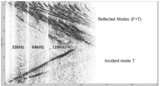
The same dataset can also be post-processed to better identify the various modes to which the sensor is sensitive generated at the two junctions of the elbow. This post-processing consists in computing a two-dimensional fast Fourier transform (FFT2D), allowing us to separate propagative modes by identifying their respective wavenumbers over the frequency spectrum of the excitation signal. Here, three excitation signals were used, made of two cycles of a sine of centre frequencies 32 kHz, 64 kHz and 128 kHz filtered by a Hanning-window. Combining the three broad bandwidths allows us to follow wavenumber variations over a frequency range from 5 kHz to 175 kHz (Figure 11):

On Fig. 11, the curve with a positive slope corresponds to the incident mode generated by the MsS system; this confirms that the first torsional mode T(0,1) is the only mode excited using this system. Curves with negative slopes correspond to reflected T(0,1) mode together with many modes created by mode conversion arising from the scattering of the incident mode at the two junctions of the elbow. This experimental result can be easily compared to the dispersion curves computed for a straight tube. An excellent fit was observed by superposing such dispersion curves onto results shown on Fig. 11 but it is rather hard to display graphically on the same figure for the present paper.

(12)

Figure 11: FFT2D of the incident mode T(0,1) and the reflected modes generated by the modes conversions in the elbow.

4.4. Comparison between numerical simulation and experimental signals

In pipe inspections by guided waves, A-scans are used to get indications about the integrity of the pipework. By interpreting this time-domain signal, information can be extracted such as the presence or not of defects and their locations, mode conversions at junctions, reflection and/or transmission coefficients and times of flight…

Here, the comparison of measured and computed A-scans is made to demonstrate the model ability to predict the complex behaviour of guided waves as they propagate and are scattered into an industrial pipework comprising an elbow. This comparison is given by figure 12:

Figure 12: comparison between experimental (blue) and simulated (black) A-scans of an inspection using T(0,1) of a pipework of 6 inches pipes comprising an elbow of 30° at 64kHz The different echoes correspond to:

(1) the reflection at the entry of the elbow T(0,1)-T(0,1)

(2) a series of mode conversions resulting from the initial mode conversion of the incident T(0,1) mode into flexural modes re-converted as torsional one, denoted by T(0,1)-F-T(0,1)

(3) reflection from the exit of the elbow of the torsional mode in the elbow similar to the T(0,1) incident mode denoted by T(0,1)-T(0,1)

(4) reflection at the end pipe T(0,1)-T(0,1)

(5) multiple scattering phenomena between the two junctions.

The comparison of the two signals shows a very good agreement in terms of number, times of flight and amplitudes of the echoes despite uncertainties with regard to elbow characteristics (irregular

(13)

curvature, wavy surface resulting from the bending process…). The multiple scattering phenomena (echoes 5) occurring after the echo of the end pipe are due to reflection and transmission between the latter and the second junction of the elbow. Further experimental validations are in progress to confirm the capabilities of the proposed model to predict these complex scattering phenomena.

5. Conclusion

A numerical model based on a modal approach and using a SAFE method coupled to a mode matching technique allows predicting the propagation and the scattering of guided waves into pipeworks comprising elbows. A single overall scattering matrix can be computed by combining propagation matrices to local scattering matrices. Interestingly, all the computations only imply meshing the guide cross-sections and solving a system of equations (FE) is only required to compute the modal basis in the various guiding parts involved (straight and curved). Thus, the overall computation allows the prediction of guided waves scattering phenomena at a low cost in terms of time and computer resources. An example of numerical parametric study of the transmission through an elbow upon frequency has been made and shows some complex scattering behaviour which highlights the importance of simulation tools for choosing the appropriate frequency for optimal inspection. Finally, an experimental study has been performed to confirm these complex diffraction phenomena produced by elbows in industrial pipeworks. Further numerical and experimental validations will be performed before integrating the developed model into the simulation software platform CIVA [3].

References

[1] T. Hayashi, K. Kawashima, Z. Sun and J.L. Rose, J. Press.Vessel Tech. 127, 322-327 (2005). [2] A. Demma, P. Cawley, M. Lowe and B. Pavlakovic, J. Press.Vessel Tech. 127, 328-335 (2005). [3] General information about the CIVA software platform can be found at www-civa.cea.fr [4] M. El Bakkali, A. Lhémery, V. Baronian and F. Berthelot, AIP Conf. Proc., 1581, 332, (2014). [5] D. Chapelle and K.-J. Bathe, The finite element analysis of shells – Fundamentals, Springer,

Berlin, 2003.

[6] F. Treyssède and L. Laguerre, J. Sound Vib. 329, 1702-1716, (2010). [7] V. Pagneux and A. Maurel, Proc. R. Soc.-A 426, 1315-1339 (2006). [8] F. Feng, J. Shen and S. Lin, Ultrasonics 52, 760-766 (2012).

[9] V. Baronian, A. Lhémery and K. Jezzine, “Hybrid SAFE/FE simulation of inspections of elastic waveguides containing several local discontinuities or defects,” in Review of Progress in QNDE, ed. by D.O. Thompson and D. E. Chimenti, AIP Conference Proceedings 1211, American Institute of Physics, Melville, NY, 2010, pp. 183-190.

[10] Guided Wave Analysis LLC website : http://www.gwanalysis.com/index.html [11] Plant Integrity Ltd website : http://www.plantintegrity.com/index.jsp