HAL Id: halshs-00676492
https://halshs.archives-ouvertes.fr/halshs-00676492
Preprint submitted on 5 Mar 2012
HAL is a multi-disciplinary open access
archive for the deposit and dissemination of
sci-entific research documents, whether they are
pub-lished or not. The documents may come from
teaching and research institutions in France or
L’archive ouverte pluridisciplinaire HAL, est
destinée au dépôt et à la diffusion de documents
scientifiques de niveau recherche, publiés ou non,
émanant des établissements d’enseignement et de
recherche français ou étrangers, des laboratoires
The public economics of increasing longevity
Pierre Pestieau, Grégory Ponthière
To cite this version:
Pierre Pestieau, Grégory Ponthière. The public economics of increasing longevity. 2012.
�halshs-00676492�
WORKING PAPER N° 2012 – 10
The public economics of increasing longevity
Pierre Pestieau
Grégory Ponthière
JEL Codes: H21, H55, I12, I13, J10
Keywords: Life Expectancy, Mortality, Public Policy
P
ARIS
-
JOURDAN
S
CIENCES
E
CONOMIQUES
48, BD JOURDAN – E.N.S. – 75014 PARIS TÉL. : 33(0) 1 43 13 63 00 – FAX : 33 (0) 1 43 13 63 10
The Public Economics of Increasing Longevity
Pierre Pestieau
yand Gregory Ponthiere
zFebruary 6, 2012
Abstract
One of the greatest success stories in our societies is that people are liv-ing longer, life expectancy at birth beliv-ing now above 80 years. Whereas the lengthening of life opens huge opportunities for individuals if extra years are spent in prosperity and good health, it is however often regarded as a source of problems for policy-makers. The goal of this paper is to examine the key policy challenges raised by increasing longevity. For that purpose, we …rst pay attention to the representation of individual preferences, and to the normative foundations of the economy, and, then, we consider the challenges raised for the design of the social security system, pension poli-cies, preventive health polipoli-cies, the provision of long term care, as well as for long-run economic growth.
Keywords: life expectancy, mortality, public policy. JEL codes: H21, H55, I12, I13, J10.
The authors are grateful to Chiara Canta for her helpful comments on this paper.
yUniversity of Liege, CORE, Paris School of Economics and CEPR. E-mail:
p.pestieau@ulg.ac.be
zEcole Normale Superieure, Paris, and Paris School of Economics. [corresponding author]
Address: Ecole Normale Superieure, 48 boulevard Jourdan, 75014 Paris, France. Tel: 0033-1-43136204. E-mail: gregory.ponthiere@ens.fr
1
Introduction
One of greatest success stories in our societies is that people are living longer than ever before. To give an idea, life expectancy at birth is now above 80 years (average for men and women), having grown by about 12 years since 1950, thanks to improvements in occupational health, health care, fewer accidents, and higher standards of living.1
This success in turn presents a huge opportunity for individuals, if extra years are spent in prosperity and good health.2 Longevity increase is however
often considered more as a source of problems than as a favorable opportunity. It may indeed have adverse implications on sustainable growth, social security systems and labor market equilibrium.
The major source of potential di¢ culties lies in the fact that existing in-stitutions and policies have been built at times where human longevity was much smaller. Hence, longevity increases may tend to make these obsolete and inadequate, inviting further changes to …t demographic tendencies. Moreover, institutions and policies may also a¤ect human longevity, and that in‡uence needs also to be taken into account in policy debates.
The purpose of this paper is to provide an overview of the e¤ects that chang-ing longevity may have on a number of public policies designed for unchanged longevity. For that purpose, we propose here to review some recent theoretical results on optimal public policy under varying longevity. The task is far from straightforward, since demographic trends do not know the scienti…c division of labor between subdisciplines. Increasing longevity raises deep challenges for the description of economic fundamentals, such as individual preferences and the social welfare criterion, as well as for the design of optimal public intervention, both in a static and a dynamic context. As a consequence, the papers and results that we survey here come from various …elds of economics, such as pub-lic economics and pubpub-lic …nance, but, also, behavioral economics, social choice theory, health economics, growth theory and development economics.
The rest of the paper is organized as follows. Section 2 presents key stylized facts about longevity increase. It appears that longevity increases over time, but at the same time remains as variable across individuals as in the past. Section 3 presents a simple lifecycle model with risky lifetime, and studies the representation of individual preferences in that context. Normative foundations are examined in Section 4. It is shown that the traditional utilitarian approach seems hardly appropriate in case of varying longevity. Then, in Section 5, we turn to the e¤ects of changing longevity on public policy for health, retirement, social security, long-term care, as well as long-run economic growth. Section 6 concludes.
1See Lee (2003) on demographic trends around the world over 1700-2000.
2On the measurement of welfare gains due to longevity increases, see Becker et al (2005),
2
Empirical facts
Let us …rst have a quick look at the phenomenon at stake: the secular rise in longevity. As this is well-known among demographers, there exist various ways to measure longevity outcomes. The most widespread indicator consists of period life expectancy at birth, that is, the average age at death reached by a cohort of newborn people, provided each cohort member faces, during his life, the vector of age-speci…c probabilities of death prevailing over some period.3
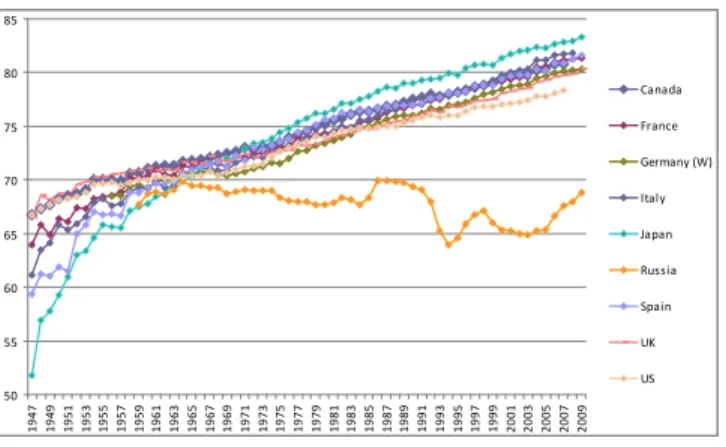
Figure 1 shows the evolution of period life expectancy at birth (for men and women) around the world, over the period 1947-2009.4
50 55 60 65 70 75 80 85 1947 1949 1951 1953 1955 1957 1959 1961 1963 1965 1967 1969 1971 1973 1975 1977 1979 1981 1983 1985 1987 1989 1991 1993 1995 1997 1999 2001 2003 2005 2007 2009 Canada France Germany (W) Italy Japan Russia Spain UK US
Figure 1: Period life expectancy at birth (total population) (years) (1947-2009)
Two important stylized facts appear on Figure 1. First, all countries under study - with the exception of Russia - have exhibited, during the last 60 years, a strong rise in life expectancy at birth. Life expectancy has, on average, grown from about 65 years in 1947 to about 82 years in 2009. Second, even if there existed signi…cant inequalities in longevity outcomes across countries in 1947, those inequalities have tended to vanish over time, except in the case of Russia, where longevity achievements are today the same as in the early 1960s. For instance, although Japan started with a life expectancy at birth of about 52 years in 1947, Japan is now at the top of longevity rankings, with an average life expectancy of 83 years. Hence, there has been a general tendency towards the lengthening of human life.
3That "period" life expectancy measure, which relies on the currently observed mortality
rates, is to be distinguished from the "cohort" life expectancy, which provides the average age at death that is actually reached by the members of a given cohort. The latter life expectancy is far less used, since this requires the death of the whole cohort under study. However, as shown in Ponthiere (2011a), the di¤erence between the expected average longevity and the actual average longevity is far from negligible.
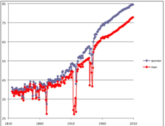
Naturally, the observed rise in total life expectancy may somewhat hide inequalities between humans, according to characteristics such as gender, geo-graphical location, education level, lifestyle, and socio-professional status. Longevity inequalities across groups within nations may be as large - if not larger - than longevity inequalities between nations. To illustrate this, Figure 2 shows the evolution of period life expectancy at birth for men and women in France.5
25 35 45 55 65 75 85 1810 1860 1910 1960 2010 women men
Figure 2: Period life expectancy at birth, men and women (years), France, 1816-2009.
The gender gap between French males and females life expectancy was equal to only 2 years in 1816 (41 years for women against 39 years for men). That gender gap has remained, during the 19th century, relatively small and constant, except at times of social troubles (for instance in years 1870-1871), during which the gap was signi…cantly larger, due to the larger involvement of men in con‡icts. But during the 20th century, the gender gap will grow continuously: it has grown from about 5 years in the mid 1930s, to about 6 years in the mid 1950s. Nowadays, the gender gap is even larger: French women live, on average, about 7 more years than French men (84.5 years for women against 77.7 years for men). That gender gap within the French economy is much more sizeable than inequalities in gender-speci…c longevity achievements between countries.
But even within a particular subpopulation, longevity inequalities may still be sizeable. Actually, life expectancy statistics provide, by de…nition, the ex-pected length of life conditionally on some vector of age-speci…c mortality rates, and, thus, focus only on the …rst moment of the distribution of longevity in the population. As such, life expectancy statistics, by focusing on the average, may tend to hide other moments of the distribution of longevity, such as the variance (2nd moment), the skewness (3rd moment) or the kurtosis (4rth moment).
In order to have a more complete view of the evolution of survival conditions over time, it may thus be most helpful to consider also the whole distribution
of the age at death, and not only the average longevity. For that purpose, the most adequate analytical tool consists of the survival curve, which shows the proportion of a cohort reaching the di¤erent ages of life. Death being an absorbing state, a survival curve is necessarily decreasing, and its slope re‡ects the strength of mortality at the age under study.
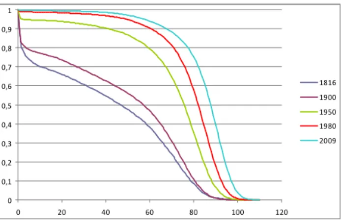
Figure 3 shows the evolution of the period survival curve in France, for women, between 1816 and 2009.6 When focusing on the left of the graph,
we see that, in comparison to the early 19th century, there has been a strong reduction of infant mortality.7 The evolution of survival curves allows us also
to measure the changes in the proportion of individuals reaching the old age: whereas only 31 % of French women could reach the age of 65 in 1816, that proportion has grown to 40 % in 1900, to 74 % in 1950, and to 92 % today.
0 0,1 0,2 0,3 0,4 0,5 0,6 0,7 0,8 0,9 1 0 20 40 60 80 100 120 1816 1900 1950 1980 2009
Figure 3: Period survival curves, women, France, 1816-2009.
Moreover, Figure 3 allows us to decompose the observed evolution of the sur-vival curves in two separate movements. On the one hand, the sursur-vival curve has tended to shift upwards. That phenomenon is known as the rectangular-ization process: a larger proportion of the cohort can reach high ages of life, even for a given maximum longevity. The rectangularization of the survival curve means that an increasingly large proportion of the population dies on an extremely short age interval. For instance, on the basis of survival conditions observed in 2009, we can measure that half of the women’s cohort will die on an age interval of about 22 years, between the age of 88 years and the age of 110 years.8 That age interval is much shorter than before, suggesting that there
is a strong concentration of deaths on a shorter and shorter age interval. The survival curve tends, over time, to become closer and closer to a rectangular,
6Sources: the Human Mortality Database (2012).
7Whereas about 17 % of women born in 1816 could not survive their …rst life-year, that
proportion decreased to about 5 % in 1950, and to 0.3 % today.
which coincides with the extreme case where all individuals would die at the same age, life becoming riskless.
Besides that rectangularization process, we have also observed another move-ment of the survival curve. The survival curves has, over time shifted not only upwards, but, also, to the right. That movement is known as the rise in limit longevity: some people can, nowadays, reach ages that could hardly have been reached in the past. That movement can be seen when focusing on the bottom-right corner of Figure 3. We can see there that the survival curve has tended, across time, to shift more and more to the right. In 1816, only 0.05 % of women could become a centenary. In 2009, that proportion is about 3.8 %, that is, 70 times the proportion prevailing in 1816.
Both the rectangularization and the rise in limit longevity explain the ob-served rise in life expectancy. Note, however, that the relative size of the two phenomena has varied over time. Whereas the rectangularization process has dominated the rise in limit longevity until the 1980s, the quasi parallel shift of the survival curve between 1980 and 2009 reveals that, over that period, there may have been some derectangularization at work. Thus, even if there has been a secular tendency towards rectangularization - and an associated reduction of the variance of the age at death - a derectangularization has recently occurred, with, as a corollary, some rise in the dispersion of longevity.9
In sum, whereas the evolution of human longevity is often summarized by the mere rise in life expectancy or average longevity, the dynamics of human longevity is more complex: a rise in life expectancy may involve either a de-crease of the risk about the length of life (as under the rectangularization), or, alternatively, an increase in the risk about the length of life (in case of derec-tangularization). Moreover, focusing on the changes in the average length of life in di¤erent countries may also somewhat tend to hide the size of longevity inequalities within countries, and the evolution of those inequalities over time.
3
A simple model
In order to study the challenges raised by those demographic trends for public policy, we will, throughout this paper, use a simple two-period model of human lifecycle. That model is deliberately kept as simple as possible, but has the virtue to capture all major aspects of life that are central to the study of the challenges raised by longevity changes.
3.1
Demography
Life is composed of, at most, two periods: the young age (…rst period) and the old age (second period). Whereas all individuals enjoy the …rst period, during which they work, consume and save some resources for their old days, only a fraction of the population will enjoy the old age. That fraction is denoted by ,
9On the measurement and causes of the rectangularization and the derectnagularization,
with 0 < < 1. On the basis of the Law of Large Numbers, can be regarded both as the probability of survival to the old age, and, also, as the proportion of the young individuals population who reach the old age, the proportion 1 dying at the end of the …rst period.
Whereas the …rst period has a length normalized to 1, the second period has a length `, with 0 < ` < 1. The motivation for introducing that second demo-graphic parameter goes as follows. As we saw above, a rise in life expectancy may correspond to either a fall or a rise in the variance of the age at death, depending on whether the survival curve shifts more upwards or more to the right. The introduction of the variable ` allows us to capture this.
Indeed, the life expectancy at birth (LE) is, in our model, equal to:
LE = (1 + `) + (1 )1 = 1 + ` (1)
Hence, a rise in life expectancy can be caused either by a rise in , meaning that the proportion of young individuals reaching the old age goes up, or by a rise in `, implying that old people live longer. In the …rst case, the variance of the age at death (V AR), equal to:
V AR = (1 + ` (1 + `))2+ (1 ) (1 (1 + `))2
= (1 ) `2 (2)
From which it appears that a rise in ` raises the variance of the length of life, whereas a rise in only raises the variance of the length of life when < 1=2, but reduces it when > 1=2.
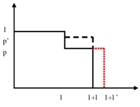
Those two movements of the survival curve are illustrated on Figure 4 below. The shift from to 0pushes the survival curve upwards, whereas the shift from
` to `0 pushes the survival curve to the right.
1 p p’
1 1+l 1+l ’
Figure 4: shifts of the survival curve in a two-period model.
Naturally, the survival curve shown on Figure 4 is quite di¤erent from the actual survival curves, shown in the previous section. But it is a simple way
to capture the various phenomena at work behind the observed rise in life ex-pectancy. The distinction between a rise in the probability of reaching the old age and a lengthening of the old age becomes, as we shall see, quite crucial when public policy is to be based on egalitarian ethical principles.10
Finally, note that the economics of increasing longevity can hardly take and ` as mere parameters, but most often regards these as the output of a health production process. The relationship between longevity outcomes and their determinants is represented by means of functional forms, which regard the demographic variable as the output of a production process using particular inputs. Those inputs can be various, and correspond to longevity determinants on which individuals have some in‡uence (e.g. physical e¤ort), or to longevity determinants on which they have no impact at all (e.g. genetic background).11
For instance, the survival probability can be regarded as the output of the following production process, modelized by the survival function ( ):
(e; "; ) (3)
where e denotes the health e¤orts made by the individual, e¤orts that can take various forms (food diet, physical exercise, etc.), while " denotes the genetic background of the individual, and accounts for the degree of knowledge of the individual ( = 0 corresponding to full myopia, whereas = 1 coincides with full knowledge). Similar functional forms can be introduced to account for the determinants of old age duration `.
3.2
Preferences
Throughout this paper, we will assume, for simplicity, that individual prefer-ences on di¤erent lives - which are here inherently risky, and, as such, can be called lotteries of life - can be represented by a function having the expected utility form. After the work by Allais (1953) on the independence axiom and its widespread violation, it is clear that this modelling of preferences is a simpli…-cation, but we will, for the sake of simplicity, rely on that simple formulation.12
Temporal welfare is represented a standard temporal utility function u ( ) that is increasing and concave in consumption. First-period consumption is denoted by c, and second-period consumption by d. Note that, given that the old age may be lived with a much worse health status, it is not uncommon to rely on state-speci…c utility function. For instance, for old-age dependency, one can use, instead of u( ), an old-age utility function H ( ), which is also increasing and concave in consumption, but with a lower welfare level ceteris paribus, i.e. u(c) > H(c) for all c level.
Assuming time-additive lifetime welfare, and normalizing the utility of death
1 0See below.
1 1See Kaplan et al (1987) on the various determinants of human longevity.
1 2See Leroux and Ponthiere (2009) for an alternative decision model, based on the moments
to zero, the expected welfare of an individual can be written as:
U = [u(c) + `u (d)] + (1 ) [u(c) + 0]
= u(c) + `u (d) (4)
in case of good health at the old age, or as:
U = u(c) + `H (d) (5)
in case of dependence at the old age.
The above formulation has the obvious advantage of simplicity: the riskiness and complexity of life is reduced to a two-term sum. However, one may wonder whether such an analytically convenient representation of individual preferences capture the key ingredients behind individual decisions. In the recent years, some strong arguments have been formulated against that formulation. The assumption of time-additivity of lifetime welfare has been speci…cally questioned by Bommier in various works (see Bommier 2006, 2007, 2010).
Bommier’s attack against the standard modelling of individual preferences relies on the attitude of individuals towards risk about the length of life. Ac-cording to Bommier, there exists a serious dissonance between, on the one hand, the actual attitude of humans in front of risk about the length of life, and, on the other hand, the predicted attitude from the standard preference modelling. More precisely, Bommier argues that individuals exhibit, in theory, "net" risk-neutrality with respect to the length of life - "net" meaning net of pure time preferences -, de…ned as the strict indi¤ erence of the agent between two lotter-ies of life with the same, constant consumption per period, and the same life expectancy. But that kind of risk neutrality is hardly plausible in real life.
It is not di¢ cult to show that the standard modelling of preferences described above involves risk-neutrality with respect to the length of life. To see this, let us compare the following two lotteries, which exhibit the same life expectancy, equal to 1 + 0:5 = 1:5:
lottery A: c = d = c, = 1 and ` = 1=2.
lottery B: c = d = c, = 1=2 and ` = 1.
The expected utility under each lottery is exactly the same, and equal to: u(c) +1
2u (c)
But are actual individuals really indi¤ erent between, on the one hand, the certainty to live an old age of length 1=2, and, on the other hand, the lottery involving a chance of 1=2 to enjoy an old age of length 1? One can have serious doubts about it: individuals are likely, when being young, to prefer the lottery A, where they are sure to live a life of length 1:5, and, thus, to escape from premature death after the young age.
According to Bommier, risk-neutrality with respect to the length of life is a far too strong postulate, which does not do justice to the actual attitude of
humans when facing risky lifetime. Therefore Bommier proposes to get rid of the time-additive utility function, and to replace it by a concave transform V ( ) of the sum of temporal utility. Expected lifetime welfare then becomes:
V [u(c) + `u (d)] + (1 )V [u(c)] (6)
with V0( ) > 0 and V00( ) < 0.
Back to the two-lottery example, the expected utility of those two lotteries is now, respectively:
V [u(c)(1:5)] for lottery A, and
0:5V [2u(c)] + 0:5V [u(c)] for lottery B.
Given the concavity of V ( ), the expected utility associated to lottery A is larger than the one associated to lottery B, in conformity with intuition.
In sum, Bommier’s critique of standard time-additive lifetime welfare func-tion illustrates how the introducfunc-tion of varying longevity in the picture signi…-cantly a¤ects how one can plausibly model human welfare. That critique is not a theoretical detail: on the contrary, it plays a signi…cant role for the under-standing and rationalization of observed choices (either health-a¤ecting choices or savings choices), and it has also tremendous consequences for public policy -in particular when consider-ing redistribution issues - as we shall discuss below.
4
Normative foundations
The extension of human lifespan requires not only a careful modelling of the lifecycle, but raises also key challenges for the speci…cation of the social objective to be pursued by governments.13
4.1
Inequality aversion
A …rst, important issue concerns the sensitivity of the social objective to the pre-vailing inequalities. True, that problem is general, and not speci…c to longevity inequalities. However, it deserves nonetheless a particular attention, since, as we shall now see, standard social objectives may lead to quite counterintuitive redistributive corollaries in the presence of inequalities in human lifespan.
To illustrate this, let us assume that longevity is purely deterministic, and that there are two types of agents in the population: type-1 agents (who rep-resent a proportion of the population) are long-lived, and type-2 agents (who represent a proportion 1 of the population) are short-lived.14 All agents
have standard, time-additive lifetime welfare. Each agent earns a wage wi in
the …rst period, supposed to be equal for the two types of agents: w1= w2= w.
1 3For simplicity, we assume all along that the total population is a continuum with a
measure equal to 1.
At the laissez-faire, type-1 agents smooth their consumption over their lifecycle, whereas type-2 agents consume their whole income in the …rst period:
c1= d1=
w
2 < c2= w
There are, in general, large welfare inequalities at the laissez-faire, because of Gossen’s First Law (i.e. concavity of temporal welfare). Indeed, under general conditions identi…ed in Leroux and Ponthiere (2010), the long-lived agent enjoys a higher lifetime welfare than the short-lived agent: u(w) < 2u w2 .15 Given the absence of risk, welfare inequalities are merely due to the Law of Decreasing Marginal Utility: long-lived agents have, ceteris paribus, a higher capacity to spread their resources on di¤erent periods, implying a higher lifetime welfare.16
Let us now see how a social planner would allocate those resources. To discuss this, let us start from a simple resource allocation problem faced by a classical utilitarian social planner, whose goal, following Bentham (1789), is to maximize the sum of individual utilities. The Benthamite social planner’s problem can be written as:
max
c1;d1;c2
[u(c1) + u(d1)] + (1 ) [u(c2)]
s.t. c1+ (1 )c2+ d1 2w
The solution is:
u0(c1) = u0(c2) = u0(d1) =
where is the Lagrange multiplier associated with the resource constraint. Sim-pli…cations yield:
c1= c2= d2=
2 3w
Classical utilitarianism implies an equalization of consumptions for all life-periods and all individuals. Hence, long-lived individuals, who bene…t from an amount of resources equal to 43w, receive twice more resources than the short-lived, who only receive 2w3 . Classical utilitarianism thus implies a redistribution from the short-lived towards the long-lived.
Note that, at the classical utilitarian optimum, the lifetime welfare inequali-ties between the long-lived and the short-lived are now larger than at the laissez-faire: instead of an inequality
2u w
2 u(w)
we now have, at the utilitarian optimum,
2u 2w
3 u
2w 3
1 5This may not be true in a very poor economy when u(w) < 0, and when u(w) > 2u w 2 .
See Leroux and Ponthiere (2010).
1 6If, on the contrary, u( ) was linear, there would be no lifetime welfare inequalities between
which is unambiguously larger. Hence classical utilitarianism implies here a double penalty of the short-lived: not only are the short-lived penalized by Nature (as they enjoy, for an equal amount of resources, a lower lifetime welfare than the long-lived at the laissez-faire), but they also su¤er from a redistribution towards the long-lived. There is one penalty by Nature, and one by Bentham.
That redistribution from the short-lived towards the long-lived is counterin-tuitive. The only way to justify it is to say that type-1 agents at the old age are di¤erent persons than type-1 agents at the young age.17 But that kind of
jus-ti…cation is far from straightforward. Another way to try to escape from that paradoxical redistribution is to opt for an alternative modelling of individual preferences, based on Bommier (2006).18 If agents’s lifetime welfare takes now
the form of a concave transform V ( ) of the sum of temporal utilities, the laissez-faire remains the same as above (as here longevity is purely deterministic), but the Benthamite social optimum is now characterized by the FOCs:
V0[u(c1) + u(d1)] u0(c1) =
V0[u(c1) + u(d1)] u0(d1) =
V0[u(c2)] u0(c2) =
where is the Lagrange multiplier associated with the resource constraint. Given the concavity of V ( ), we now have:
c1= d1< c2
that is, the short-lived has now a higher consumption per period than the long-lived. Hence, lifetime welfare inequalities are here reduced in comparison to classical utilitarianism. In some sense, concavifying lifetime welfare is formally close to shifting from classical towards more inequality-averse utilitarianism, as suggested, among others, by Atkinson.19
Note, however, that the concavi…cation of lifetime utilities through the trans-form V ( ) only mitigates the tendency of utilitarianism to redistribute from the short-lived towards the long-lived, but does not, in general, su¢ ce to reverse the direction of redistribution.20 An alternative solution is thus needed. One
rem-edy, based on Broome’s (2004) attempt to provide a value to the continuation of life, consists of monetizing the welfare advantage induced by a longer life, and to count it as a part of the consumption enjoyed by the long-lived. As shown by Leroux and Ponthiere (2010), that solution is close to the Maximin solution, that is, a social welfare function à la Atkinson, but with an in…nite inequality aversion. Another remedy is the possibility of giving more social weight to the short-lived individuals relative to the long-lived ones, in such a way that in the …rst-best there would be no transfer from the …rst to the second.
1 7See Par…t (1984) on di¢ culties to account for a constancy of human identity over a
lifecycle.
1 8On the redistributive consequences of risk-aversion with respect to the length of life, see
Bommier et al (2011a, 2011b).
1 9See Atkinson and Stiglitz (1980), p. 339-340. 2 0On this, see Leroux and Ponthiere (2010).
4.2
Responsibility and luck
As shown above, longevity inequalities raise serious challenges to policy-makers even under standard consequentialist social objectives (like utilitarian social objectives). But beyond individual outcomes in terms of longevity and con-sumption, one may argue that a reasonable social objective should also pay attention to how those outcomes are reached. In our context, this amounts to examine the reasons why some individuals turn out to be short-lived, whereas others turn out to be long-lived.
The underlying intuition, as advocated by Fleurbaey (2008), is the follow-ing.21 True, the idea of responsibility has remained surprisingly absent from important strands of normative thinking in political philosophy and welfare eco-nomics. However, as soon as we are living in free societies, where free individuals make decisions about, for instance, the goods they consume, the activities they take part in, the job for which they apply, etc., it seems hardly plausible to leave responsibility issues aside. Responsibility is a necessary consequence of any substantial amount of freedom. As such, whatever theorists think about responsibility or not, responsibility is a parcel of any free society.
This is the reason why late 20th century egalitarian theories, such as the ones advocated by Rawls (1971), Dworkin (1981a, 1981b), or Cohen (1993), are all, at least to some extent, relying on a distinction between what characteristics of situations are due to pure luck, and what characteristics are, on the contrary, due to individual choices, and, as such, involve their responsibility. That dis-tinction between luck characteristics and responsibility characteristics is crucial for policy-making. According to Fleurbaey (2008), welfare inequalities due to luck characteristics are ethically unacceptable, and, as such, invite a compensa-tion: this is the underlying intuition behind the compensation principle ("same responsibility characteristics, same welfare"). However, welfare inequalities due to responsibility characteristics are ethically acceptable, and, thus, governments should not interfere with the latter type of inequalities: this is the natural reward principle ("same luck characteristics, no intervention").
The distinction between luck characteristics and responsibility characteris-tics is most relevant for the study of longevity inequalities. As shown by Chris-tensen et al (2006), the genetic background of individuals explains between 1/4 and 1/3 of longevity inequalities within a cohort.22 Hence, given that
individu-als do not choose their own genetic background, a signi…cant part of longevity inequalities lies outside their control. However, individuals can have also a sig-ni…cant in‡uence on their survival chances, through their lifestyle. As shown by Kaplan et al (1987) longitudinal study in California, individual longevity depends on eating behavior, drinking behavior, smoking, sleep patterns and physical activity.
It follows from all this that longevity is partly a luck characteristic of the
2 1See Fleurbaey (2008), p. 1-9.
2 2That study is based on the comparison of longevity outcomes among pairs of monozygotic
twins and pairs of dizygotic twins. The correlation of longevity outcomes is much larger among the former twins, who share (almost) the same genetic background.
individual, and partly a responsibility characteristic. That double-origin of longevity inequalities leads us to a problem that is now well known in the com-pensation literature (see Fleurbaey and Maniquet 2004): it is impossible, under general conditions, to provide compensation for a luck characteristic without, at the same time, reducing inequalities due to responsibility characteristics. Hence, a choice is to be made between compensation and natural reward.
To illustrate this, consider the simple case where there are two groups of agents i = 1; 2, whose old-age longevity `i is a function of genes "i and health
e¤orts ei. Those agents di¤er on two aspects. On the one hand, agents of
type-1 have better longevity genes than individuals of type-2. On the other hand, type-1 individuals have a lower disutility from e¤ort than type-2 individuals. In that setting, the genetic background is a circumstance or luck characteristics, whereas the disutility of e¤ort is a responsibility characteristics.23 For simplicity,
the longevity is assumed to be given by: `i "i` (ei)
with `0( ) > 0, and `00( ) < 0. We assume "1> "2. The disutility of e¤ort is:
vi(ei) iv(ei)
with v0( ) > 0, and v00( ) > 0. We assume: 1< 2.
At the laissez-faire, agents solve the problem:24 max
ci;di;ei
u(ci) iv(ei) + "i` (ei) u(di)
s.t. ci+ "i` (ei) di w
The FOCs yield, for agents of type i = 1; 2: ci = di
iv0(ei) = "i`0(ei) [u(di) u0(di)di]
Given "1> "2 and 1 < 2, type-1 agents make, ceteris paribus, more e¤ort
than type-2 agents. If agents had the same genes ("1= "2), it would still be the
case that type-1 agents make more e¤ort than type-2 agents. Alternatively, if they all had the same disutility of labour, type-1 agents would still make more e¤orts (because of better genes).
Comparing their lifetime welfares, we expect that type-1 agents have, thanks to their better genes and lower disutility of e¤ort, a higher welfare. Are those welfare inequalities acceptable? Yes, but only partly.
Note that, if all agents had the same disutility of e¤ort (if 1= 2= ),
type-1 agents would still get a higher welfare, thanks to their better genes. Hence, the compensation principle ("same responsibility, same welfare") would require to redistribute from type-1 towards type-2, to obtain the equality:
u(c1) v(e1) + "1` (e1) u(d1) = u(c2) v(e2) + "2` (e2) u(d2)
2 3We follow Fleurbaey (2008), who treats preferences as responsibility characteristics. 2 4Here again, we assume that the two agents have the same wage in the …rst period, w.
As "1 > "2, we expect c1 < c2 and/or d1 < d2: some monetary compensation
should thus be given to type-2 agents.
If all agents had equal genes (if "1 = "2= "), type-1 agents would still be,
thanks to a lower disutility of e¤ort, better o¤ than type-2 agents. But the principle of natural reward ("equal luck, no intervention") would regard those inequalities as acceptable, since these are not due to luck:
u(c1 ) 1v(e1 ) + "` (e1 ) u(d1 ) > u(c2 ) 2v(e2 ) + "` (e2 ) u(d2 )
The problem is that the need to compensate for inequalities due to luck characteristics may clash with the non-interference on inequalities due to re-sponsibility characteristics. To see this, suppose reference disutility = 1 and
reference genes " = "1.25 Then, the above conditions become:
u(c1) v(e1) + "` (e1) u(d1) = u(c2) v(e2) + "2` (e2) u(d2)
u(c1 ) v(e1 ) + "` (e1 ) u(d1 ) > u(c2 ) 2v(e2 ) + "` (e2 ) u(d2 )
We see that those two conditions are, in some cases, incompatible. Indeed, the LHS of the two conditions are the same. Hence, if "1` (e2 ) u(d2 ) "2` (e2) u(d2) >
2v(e2 ) 1v(e2), we obtain a contradiction. Thus a given allocation may fail
to satisfy both the compensation principle and the natural reward principle. Such a con‡ict between compensation and reward is not uncommon when there is no separability between the contributions of e¤ort and luck to individual payo¤s.26 This is the case in our example, where type-1 agents, who have better genes than type-2 agents, make also more e¤orts. Hence it is impossible to give them the reward for their e¤orts, and, at the same time, to compensate type-2 agents, since the latter compensation goes against rewarding e¤orts.
4.3
Ex ante
versus ex post equality
In the previous subsections, we deliberately ignored risk, in order to keep our analysis as simple as possible. However, the risky nature of lifetime raises ad-ditional di¢ culties regarding the choice of a social objective, as we shall now see. The problem consists of adopting the perspective that is most relevant for comparing several distributions of individual outcomes (including longevities).
As stressed by Fleurbaey (2010), there exists a dilemma between two ap-proaches to normative economics in presence of risk. One can adopt an ex ante approach, which evaluates the distribution of individual expected outcomes be-fore the uncertainty about the state of nature is revealed, or, alternatively, an ex post approach, which evaluates the distribution of individual outcomes that are actually prevailing after uncertainty has disappeared.
Note that, in some circumstances, there is no opposition between the two approaches. When a government adopts, as a social objective, average utilitar-ianism, and when all agents are ex ante perfectly identical, the Law of Large
2 5The choice of reference levels on all relevant characteristics is not always neutral, but is a
necessary task to be able to discuss compensation and reward concerns.
Numbers guarantees the equivalence between, on the one hand, the allocation of resources maximizing the ex ante (expected) lifetime welfare of individuals, and, on the other hand, the allocation maximizing the average lifetime welfare ex post in the population.27
However, once one adopts a more egalitarian perspective, the ex ante and an ex post approaches to normative economics are no longer equivalent, and the associated social optima di¤er strongly. To see this, let us consider a simple allocation problem, in a context where all individuals, who are ex ante identical, can turn out to have either a short or a long life.28 Individuals face a life
expectancy 1 + . At the laissez-faire, each agent solves the problem:29
max
c;d u(c) + u(d)
s.t. c + d w
The FOCs imply:
c = d = w
1 + where 1
1+ is the return of the annuity.
Take now the social planning problem of a planner who has, as an objective, to maximize the minimum expected lifetime welfare in the population. Given that all individuals are, ex ante, identical, the solution to that ex ante egalitarian approach coincides with the laissez-faire.
Compare now that solution with the one of an alternative planning problem: the maximization of the minimum ex post lifetime welfare. That problem, which was studied by Fleurbaey et al (2011), can be written as:
max
c;d minfu(c) + u(d); u(c)g
s.t. c + d w
The solution involves several cases. In each case, c denotes the welfare-neutral consumption level, such that u(c) = 0. Restricting ourselves to the case where c = 0, we have
c > d = c = 0
The solution of the ex post egalitarian planning problem is very di¤erent from the one of the ex ante problem. The underlying intuition is that, in order to minimize welfare inequalities between long-lived and short-lived, one must give to the surviving old what makes them exactly indi¤erent between further life and death, that is, the welfare-neutral consumption level c. Any euro left at the old age beyond that welfare-neutral consumption level prevents the minimization of welfare inequalities: redistributing it to the young age would raise the welfare of the short-lived, and, hence, reduce welfare inequalities.
2 7See Hammond (1981) on that equivalence. 2 8For simplicity, we assume ` = 1.
2 9We assume here a perfect annuity market for each class of risk. Its implications for policy
In the light of this, there exists, in a context of risky longevities, a signi…cant discrepancy between what recommends an ex ante egalitarian social objective, and what recommends an ex post egalitarian social objective. Whereas the for-mer optimum coincides with the laissez-faire in case of ex ante identical agents, the latter optimum recommends a serious departure from common sense, by advocating a lifecycle that makes individuals indi¤erent between living long or not.30 Whereas that dilemma between ex ante and ex post approaches to
nor-mative economics is very general, and thus not speci…c at all to the demographic environment under study, it cannot be overemphasized here that this dilemma occurs in a particularly acute way in the present context, since inequalities in life expectancy are very small in comparison to inequalities in actual lifespans.
5
Implications for social policy
5.1
Free-riding on longevity-enhancing e¤ort
Should the government subsidize longevity? At …rst glance, that question sounds more provocative than relevant, as this seems to question something unques-tionable. There can be no doubt that the large rise in longevity that we are witnessing is a good thing. Various preferences-based indicators of standards of living taking longevity into account con…rm that intuition.31 It is thus tempting
to conclude that governments should promote longer lives.
There are however some reasons why the government should intervene neg-atively, and tax longevity, contrary to the common sense. The …rst reason is linked to the annuitization of collective or individual savings when life duration is uncertain and endogenous. As shown by Davies and Kuhn (1992) and by Becker and Philipson (1998), individuals do not necessarily take into account, in their longevity-related choices, the negative e¤ect that these choices can have on the cost of annuities, and, thus, on the return of their savings. As a conse-quence, agents may tend to invest too much in their health in comparison with what would maximize lifetime welfare. This applies to private saving but also to a Pay-As-You-Go pension scheme. To illustrate that, we take our two period example with life time utility:
U = u(w s e) + (e)u(s (1 + r)= (e) + (1 + n)= (e)) (7)
where r is the market interest rate, 1+ris the return of an actuarilly fair annuity,
and n is the rate of population growth, while is the payroll tax that …nances the pension of the contemporary retirees having survived. Optimal saving s is given by:
u0(c) = u0(d)(1 + r) (8)
The choice of health expenditure is given by:
0(e)u(d) = u0(d)(1 + r) + 0(e)u0(d)d (9)
3 0Similar departures would be obtained in more complete models, with unequal life
ex-pectancies, endogenous labour supply, or endogenous survival depending on e¤ort.
The LHS is the bene…t from an increased survival probability. The …rst term of the RHS gives the direct budgetary cost of health spending. The second term of the RHS give the depressing e¤ect of longevity enhancing spending on both private saving and public pension. Individuals do not internalize this e¤ect in their choice and this calls for a corrective pigouvian tax on health spending. As shown by Eeckhoudt and Pestieau (2009), this latter expression can be interpreted in terms of some sort of risk aversion measured by the fear of ruin.
Finally, note that, while Davies and Kuhn (1992) as well as Becker and Philipson (1998) cast their analysis in a static setting, some recent papers study optimal health investment in a dynamic environment. For instance, Pestieau et al (2008) study the optimal health spending subsidy in an economy with a Pay-As-You-Go pension system with a …xed replacement ratio, and show that health spending may exceed what is socially optimal, inviting the taxation of health e¤orts. Another reason for taxing health spending pertains to the Tragedy of the Commons. As shown by Jouvet et al (2010), given that the Earth is spatially limited (like a spaceship), ever increasing longevity can also be a problem, inviting, here again, a pigouvian tax.
5.2
Optimal policy and heterogeneity
When individuals are heterogeneous on longevity-a¤ecting characteristics, there are other important dimensions a¤ecting the issue of taxing or subsidizing longevity. To examine that issue, Leroux et al (2011a, 2011b) study an econ-omy where people di¤er in three aspects: longevity genes, productivity and myopia. Within that setting, they apply the analytical tools of optimal taxa-tion theory to the design of the optimal subsidy on preventive behaviors, in an economy where longevity depends on preventive expenditures, on myopia and on longevity genes following equation (3).
Public intervention can be here justi…ed on two grounds: corrections for misperceptions of the survival process and redistribution across both earnings and genetic dimensions. The optimal subsidy on preventive expenditures is shown to depend on the combined impacts of misperception and self-selection. It is generally optimal to subsidize preventive e¤orts to an extent depending on the degree of individual myopia, on how productivity and genes are correlated, and on the complementarity of genes and preventive e¤orts in the survival function. If richer individuals tend to invest more in longevity-enhancing activities, it can be socially optimal to tax them in a second best setting wherein the social planner observes neither productivity nor longevity genes.
In other words, the taxation of longevity-enhancing activities can serve as an indirect way to achieve social welfare maximization in the context of asym-metric information. Whereas the redistributive e¤ect is ambiguous as to taxing or subsidizing, the presence of myopia clearly calls for a subsidy. Clearly, if individuals, because of their ignorance or myopia, do not perceive the deferred e¤ect that their savings and health care choices may have on their future con-sumption and their longevity, then such an imperfection of behavior invites some
governmental correction against individual underinvestment in health.
Note that the design of the optimal policy is even trickier when risk-taking agents di¤er as to their attitudes towards their past health-related choices. As discussed in Pestieau and Ponthiere (2012), the consumption of sin goods, such as alcohol and cigarettes, may lead some individuals - but not all - to regret their choices later on. Hence, whereas the decentralization of the …rst-best optimum would only interfere with the behaviors that agents will regret ex post, asymmetric information and redistributive concerns imply interferences not only with myopic behaviors, but, also, with impatience-based (rational) behaviors.32
Finally, whereas most of the literature on optimal taxation under heterogene-ity focuses on economies with a …xed partition of the population into di¤erent types, allowing that partition to vary introduces additional taxation motives. As shown by Ponthiere (2010) in a dynamic model with unequal longevities due to distinct lifestyles, public intervention may interact with the socialization process, and, hence, a¤ect the long-run composition of the population. Such intergenerational composition e¤ects need to be taken into account when con-sidering the optimal public intervention, as there may exist con‡icts between social welfare maximization under a …xed composition of the population and social welfare maximization under a varying composition.
5.3
Retirement and social security
Special pension provisions such as early retirement for workers in hazardous or arduous jobs are the subject of a great deal of debate in the pension arenas of many OECD countries. Such provisions are historically rooted in the idea that people who work in hazardous or arduous jobs –say, underground mining – merit special treatment: such type of work increases mortality and reduces life expectancy, thus reducing the time during which retirement bene…ts can be enjoyed. This results in such workers being made eligible for earlier access to pension bene…ts than otherwise available for the majority of workers.
In a recent paper, Pestieau and Racionero (2012) discuss the design of these special pension schemes. In a world of perfect information, earlier retirement could be targeted towards workers with lower longevity. If there were a perfect correlation between occupation and longevity, it would su¢ ce to have speci…c pension provisions for each occupation. Unfortunately, things are less simple as the correlation is far from being perfect. Granting early retirement to an array of hazardous occupations can be very costly. Government thus prefers to rely on disability tests before allowing a worker to retire early. Another argument for not having pension provisions linked to particular occupations is the political impossibility of cancelling them if these occupations become less hazardous.
To analyze this issue, they adopt a simple setting with two occupations and two levels of longevity. All individuals have the same productivity but those with the hazardous occupation face a much higher probability to have a short
3 2Various theoretical papers examine the optimal taxation of sin goods under
time-inconsistency. See, among others, Gruber and Koszegi (2000, 2001), as well as O’Donoghe and Rabin (2003, 2006).
life than those who have a secure occupation. The health status that leads to a high or a low longevity is private information and known to the worker at the end of the …rst period. Before then everyone is healthy.
Individuals are characterized by their health status that leads to either longevity `S or `L with `S < `L (where L stands for long and S for short)
and by their occupation, 1 for the harsh one and 2 for the safe one. Individuals retire after z years of work in the second period; they then know their health status ` that is represented in v(z; `), their disutility for working z years given that their longevity is `. We assume that v ( ) is strictly convex in z and that the marginal disutility of prolonging activity decreases with longevity.
The individual utility is given by:
U = u(c) + `u(d) v(z; `) (10)
with a budget constraint equal to
c + `d = w(1 + z): (11)
Assuming that there is no saving, the only choice is z that is given by
u0(d)w v0(z; `) (12)
From this FOC, one obtains that dz=d` > 0 if dv0=d` < 0, which is reasonable.
We have thus 4 types of individuals denoted by kj with k = L; S and j = 1; 2. By de…nition, the probability of having a long life is higher in occupation 2, than in occupation 1, namely 2 > 1. In a world where 1 = 0 and 2 = 1, the problem of a central planner would be easy. If he maximizes the
sum of individual utilities, the social optimum would be given by the equality of consumption across individuals and periods and by z1 > z2. In the reality,
however, we do not have those extreme cases; some workers can experience health problems even in a rather safe occupation and workers can have a long life even holding a hazardous job. If health status were common knowledge, the …rst best optimum would still be achievable. If it is private information, one has to resort to second best schemes. Tagging is a possibility. Assume that 1> 0
and 2= 1. Then it may be desirable to provide a better treatment to type L1
than to type L2. This is the standard horizontal inequity outcome that tagging generates. An alternative (or a supplement) to tagging might be disability tests. If these were error-proof and free, they could lead to the …rst best. Otherwise, a second-best outcome is unavoidable.
In the Pestieau / Racionero approach, the focus is on ex ante welfare. In Fleurbaey et al (2012) the ex post and the ex ante optimum are compared. It appears that the age of retirement will be higher in the ex post optimum than in the ex ante one. The intuition goes as follows. In the ex post approach, the focus is on the individual who ends up with short life, which leads to low saving, if any. Those who survive will have to work longer in the second period as they have less saving than they would have in the ex ante approach.
5.4
Long term care social insurance
One of the main rationale for social insurance is redistribution. Starting with the paper of Rochet (1991) the intuition is the following. We have an actuarially fair private insurance and the possibility of a social insurance scheme to be developed along an income tax. If there were no tax distortion, the optimal policy is to redistribute income through income taxation and let individuals purchase the private insurance that …ts their needs. If there is a tax distortion and if the probability of loss is inversely correlated with earnings, then social insurance becomes desirable. Given that low-income individuals will bene…t in a distortionless way from social insurance more than high-income individuals, social insurance dominates income taxation. In that reasoning, moral hazard is assumed away but the argument remains valid with some moral hazard.
While the above proposition applies to a number of lifecycle risks, it does not apply to risks whose probability is positively correlated to earnings, typically long term care (LTC). Dependence is known to increase with longevity and longevity with income. Consequently, the need for LTC is positively correlated with income, and Rochet’s argument implies that a LTC social insurance would not be desirable. This statement does not seem to …t reality, where we see the needs for LTC at the bottom of the income distribution. Where is the problem? First, we do not live in world where income taxation is optimal. Second, even if we had an optimal tax policy, it is not clear that everyone would purchase a LTC insurance. There is quite a lot of evidence that most people understate the probability and the severity of far distanced dependence.33 This type of
myopia or neglect calls for public action. Finally, private LTC insurance is far from being actuarially fair; loading costs are high (see Cutler 1993, Brown and Finkelstein 2004a) and lead even farsighted individuals to keep away from private insurance: low income individuals will rely on family solidarity or social assistance and high income individuals on self-insurance.34
Cremer and Pestieau (2011) study the role of social LTC insurance in a setting, which accounts for the imperfection of income taxation and private insurance markets. Policy instruments include public provision of LTC as well as a subsidy on private insurance. The subsidy scheme may be linear or nonlinear. For the nonlinear part, they look at a society made of three types: poor, middle class and rich. The …rst type is too poor to provide for dependence; the middle class type purchases private insurance and the high income type is self-insured. Two crucial questions are then: (1) at what level LTC should be provided to the poor? (2) Is it desirable to subsidize private LTC for the middle class?
Interestingly, the results are similar under both linear and nonlinear schemes. First, in both cases, a (marginal) subsidy of private LTC insurance is not
de-3 de-3According to Kemper and Murtaugh (1997), a person of age 65 has a 0.43 probability
to enter a nursing home. Nonetheless, as shown by Finkelstein and McGarry (2003), about 50 % of the population with an average age of 79 years reports a sub jective probability of institutionalization within 5 years equal to 0.
3 4Empirical papers on the origins of the LTC insurance puzzle in the U.S. include Brown
and Finkelstein (2004b) and Brown et al (2006). Courbage and Roudaut (2008) examine that issue on the basis of SHARE data for France.
sirable. As a matter of fact, private insurance purchases should typically be taxed (at least at the margin). Second, the desirability of public provision of LTC services depends on the way the income tax is restricted. In the linear case, it may be desirable only if no demogrant (uniform lump-sum transfer) is available. In the nonlinear case, public provision is desirable when the income tax is su¢ ciently restricted. Speci…cally, this is the case when the income is subject only to a proportional payroll tax while the LTC reimbursement policy can be nonlinear.
5.5
Preventive and curative health care
Consider now an economy where individuals live for two periods: the …rst one is of length one and the second has a length ` that depends on private investment in health in the second period and on some sinful consumption in the …rst period. It is likely that some people do not perceive well (out of myopia or ignorance) the impact of their lifestyle on their longevity.
Within this framework, Cremer et al (2012) study the optimal design of taxation. As expected, sin goods should be taxed, but curative health spending should not necessarily be subsidized, particularly when there is myopia. They distinguish between two cases, according to whether or not individuals acknowl-edge and regret their mistake in the second period of their life. When individuals acknowledge their mistake at the start of the second period, there is no need to subsidize health care, but a subsidy on saving is desirable.
To illustrate this, let us consider the problem of an individual who does not perceive the impact of some sin good x on his longevity. The longevity function can be written as `( x; e), where equals 1 for a rational individual, and 0 for a myopic one, while e denotes the curative health spending. The social planner - or a rational individual - would maximize:
U = u(c) + u(x) + `(x; e)u(d) subject to the resource constraint:
c + x + e + `(x; e)d = w
A myopic individual would maximize in the …rst period: U = u(w s x) + u(x) + `(0; e)u ((s e)=`(0; e))
So doing, the individual is likely to save too little or too much. Consuming more x than it is optimal and expecting to spend less e decreases saving. Expecting to live longer fosters saving. In the second period, given x, he allocates this saving between d and e so as to maximize:
`(x; e)u((s e)=`(x; e))
It can be shown that, to implement the …rst-best, the government has to subsidize saving and tax the sin good. So doing the myopic individual will
reach the second period with the right amount of sin good and enough saving to optimally choose both d and e.
Assume now that the individual persist in his mistake and chooses e keeping ignoring the e¤ect of e¤ort e on longevity. In that case the government has to subsidize e to reach the …rst best allocation. Naturally, with heterogeneity in both w and , public policy would be more di¢ cult to implement and more complex to design. Restoring the …rst best would then be mission impossible.
5.6
Long-run economic growth
Given that life expectancy determines human life horizon, this is most likely to in‡uence decisions a¤ecting economic growth: savings, education, retirement, and fertility. Growth theorists studied the impact of varying longevity in over-lapping generations (OLG) models, and assumed either that life expectancy is exogenous, or that it can be a¤ected by education, health investment or lifestyle. Those variables being strongly in‡uenced by governments, that literature is di-rectly relevant for the long-run public economics of varying longevity.
Starting with the …rst approach, Ehrlich and Lui (1991) developed a three-period OLG model in which human capital is the engine of growth, and where generations are linked through material and emotional interdependencies within the family. Agents are both consumers and producers, who invest in their chil-dren to achieve both old-age support and emotional grati…cation, and material support from children is determined through self-enforcing implicit contracts. Ehrlich and Lui showed that the higher life expectancy is, the higher education investment in children is, leading to a lower fertility and a higher output per head. The link between life expectancy, fertility and growth is also studied by Zhang et al (2001), in an OLG economy with a Pay-As-You-Go pension system. They showed that the decline in mortality can a¤ect fertility, education, and, hence, economic growth, positively or negatively, depending on the form of pref-erences.35 Boucekkine et al (2009) also focused on the relation between fertility
and mortality, but in the context of epidemics, and showed that a rise in adult mortality has an ambiguous e¤ect on both net and total fertility, while a rise in child mortality increases total fertility, but leaves net fertility unchanged.
The impact of changes in life expectancy on human capital accumulation and growth was studied by Boucekkine et al (2002) in a vintage human capital model, where each generation of workers constitutes a distinct input in the production process.36 Here again, the impact of a rise in life expectancy on
growth is ambiguous. Three e¤ects are at work. First, a rise in longevity raises the "quantity" of workers, leading to a higher production. Second, a rise in longevity favors investment in education, following the Ben Porath e¤ect (see Ben Porath 1967), inducing also higher production. Third, the fall of mortality increases the average age of the working population, which may have a negative
3 5In a related paper, Zhang and Zhang (2005) show, under a logarithmic utility in leisure
and the number of children, that rising longevity reduces fertility, but raises saving, schooling time and economic growth at a diminishing rate.
e¤ect on productivity and growth. Boucekkine et al (2002) argued that, in a developing economy, the two positive e¤ects dominate the third, negative e¤ect, whereas the opposite may prevail in advanced economies.37
The impact of life expectancy on savings and physical capital accumulation was recently studied by D’Albis and Decreuse (2009), who showed that parental altruism and life expectancy favor capital accumulation, and compared the as-sociated intertemporal equilibrium with the in…nite-horizon Ramsey model. To evaluate the joint e¤ect of PAYGO pensions and longevity on long-term growth, Andersen (2005) studied an OLG model with uncertain length of life and endo-geneous retirement age. The main results is that uncertain longevity implies a retirement age that is proportional to average longevity and increases the need to shift from a PAYG system to a fully funded one. The impact of mortality changes on the retirement decision was also studied by d’Albis et al (2012), who showed that a mortality decline at an old age leads to a latter retirement age, whereas a mortality decline at a younger age may lead to earlier retirement.
Turning now to models assuming endogenous longevity, a seminal paper is Chakraborty (2004), who introduced risky lifetime in a two-period OLG model with physical capital accumulation, assuming that the survival conditions are increasing in health expenditures. In that model, high-mortality societies can-not grow fast, since lower longevity discourages saving and investment such as education. Regarding long-run dynamics, Chakraborty showed, under a log-arithmic temporal utility function, and a Cobb-Douglas production function, that there exists, when the elasticity of output with respect to capital is smaller than 1/2, a unique and locally stable stationary equilibrium. Chakraborty also introduced, in a second stage, human capital accumulation through education in the …rst period, and showed that countries di¤ering only in health capital do not converge to similar living standards. A low-mortality economy always invests more intensively in skill at a higher rate and thereby augments its health capital at a faster pace. As a result, it consistently enjoys a higher growth rate along its saddle-path than economies with higher mortality risks.38
Following Chakraborty (2004), various dynamic models with endogenous mortality were developed.39 Bhattacharya and Qiao (2005) focused on a two-period OLG model where both public and private health spending a¤ect life ex-pectancy. They show that, when those two health spendings are complementary in the production of survival, the economy is exposed to aggregate endogenous ‡uctuations and possibly chaos.40 De la Croix and Sommacal (2009) studied the
interplay between medicine investment, scienti…c knowledge formation and life
3 7On the link between life expectancy and education, de la Croix et al (2008) showed that
about 20 % of education rise in Sweden (1800-2000) arised thanks to life expectancy growth.
3 8Following Chakraborty, Finlay (2005) studied how investments in health and in education
compete as ways allowing economies to escape from poverty traps.
3 9Chakraborty and Das (2005) studied the impact of endogenous mortality on inequalities.
On a more normative side, de la Croix and Ponthiere (2010) examined optimal capital ac-cumulation in a Chakraborty-type economy. The relation between optimal fertility rate and optimal survival rate is explored in de la Croix et al (2012).
4 0Long-run cyclical dynamics is also studied by Ponthiere (2011b) in a model where life
expectancy growth in an OLG framework. Ponthiere (2009) examined, in a two-period OLG model with endogenous and `, the conditions under which the rectangularization is followed by a derectangularization of the survival curve. Chen (2009) studied the relationship between health capital, life expectancy and economic growth in a two-period OLG model where individuals can invest in their own health capital, which in‡uences their life expectancy, and, hence, economic growth. Finally, Boucekkine and La¤argue (2010) explored the dis-tributional consequences of epidemics in a three-period OLG economy where health investments are chosen by altruistic parents, and show that epidemics can have permanent e¤ects on the size of population and output level.
In the recent years, various models were built to explain the "demographic transition", i.e. the shift from a regime with high mortality and high fertility to a regime with low mortality and low fertility. Blackburn and Cipriani (2002) studied a three-period OLG setting where both mortality and fertility are func-tions of human capital. They showed that, under standard functional forms for production and utility, the chosen education is increasing in life expectancy (i.e. Ben Porath e¤ect), while early fertility is decreasing with it. Several stationary equilibria exist: one with high fertility and low life expectancy; another one with low fertility and high life expectancy, as well as an intermediate unstable equilibrium. Hence, an economy that starts up with poor situation may be des-tined to remain poor (so called poverty trap), unless there are major exogenous shocks. Initial conditions matter for demographic transition or stagnation.
Various alternative economic models of the demographic transition have been developed in the recent years. Galor and Moav (2005) provided an explanation of the demographic transition that is based on a shift in evolutionary advantage, from the "short-lived / large fertility" type to the "long-lived / low fertility" type, which occurred as a consequence of total population growth. The interplay between education, fertility and longevity is further studied by Cervelatti and Sunde (2005, 2011) and by de la Croix and Licandro (2012).41
5.7
Miscellenaous issues
Poverty alleviation and health policy Survival chances vary quite a lot at the old age, according to various characteristics (gender, geographic location, etc.). One of those characteristics is the income: longevity is, ceteris paribus, increasing in individual income.42 As argued by Kanbur and Mukherjee (2007),
the positive income / longevity relationship has a quite embarrassing corollary for the measurement of poverty at the old age. The reason is that, under income-di¤erentiated mortality, standard poverty measures capture not only the "true" poverty, but, also, the interferences or noise caused by survival laws. Indeed, income-di¤erentiated survival laws select proportionally fewer poor persons than non-poor persons. Hence, poor persons are "missing", in a way similar to the "missing women" phenomenon studied by Sen (1998).
4 1Another study of the demographic transition is Yew and Zhang (2011), who show that
social security reduces fertility and raises longevity, capital intensity and output per worker.