HAL Id: tel-00667491
https://tel.archives-ouvertes.fr/tel-00667491
Submitted on 7 Feb 2012
HAL is a multi-disciplinary open access
archive for the deposit and dissemination of
sci-entific research documents, whether they are
pub-lished or not. The documents may come from
teaching and research institutions in France or
L’archive ouverte pluridisciplinaire HAL, est
destinée au dépôt et à la diffusion de documents
scientifiques de niveau recherche, publiés ou non,
émanant des établissements d’enseignement et de
recherche français ou étrangers, des laboratoires
instrument and Monte Carlo modelling of the hydrogen
exosphere
Mea Simon Wedlund
To cite this version:
Mea Simon Wedlund. MERCURY In-flight calibration of the PHEBUS UV instrument and Monte
Carlo modelling of the hydrogen exosphere. Planetology. Université Pierre et Marie Curie - Paris VI,
2011. English. �NNT : 2011PA066114�. �tel-00667491�
MERCURY
In-flight calibration of the PHEBUS UV instrument
&
Monte Carlo modelling of the hydrogen exosphere
MEA SIMON WEDLUND
Laboratoire Atmosph`
eres, Milieux, Observations Spatiales
Monograph for the degree of Doctor Scientiarum
Astronomy and Astrophysics
Universit´
e Pierre et Marie Curie
Astronomy and Astrophysics
Monograph for the degree of
Doctor Scientiarum
Universit´
e Pierre et Marie Curie
MERCURY
In-flight calibration of the PHEBUS UV
instrument
&
Monte Carlo modelling of the hydrogen exosphere
MEA SIMON WEDLUND
Laboratoire Atmosph`
eres, Milieux, Observations Spatiales
Publicly presented and defended
3 May 2011
Jury
Dr. Bruno Sicardy
LESIA, Meudon
President of Jury
Dr. Helmut Lammer
IWF, Graz
Referee
Dr. Iannis Dandouras
CESR, Toulouse
Referee
Dr. Gabriele Cremonese
INAF, Padova
Examiner
Dr. Mathieu Barth´elemy
LPG, Grenoble
Examiner
Dr. Eric Chassefi`ere
IDES, Orsay
Supervisor
Dr. Franςois Leblanc
LATMOS, Paris
Advisor
prepared at Service d’A´eronomie (SA), Laboratoire Atmosph`eres, Milieux,
Observations Spatiales (LATMOS) and Universit´e Pierre et Marie Curie
(UPMC), Paris, France.
Astronomie et Astrophysique
Th`
ese pour obtenir le grade de
DOCTEUR
de l’Universit´
e Pierre et Marie Curie
MERCURE
Calibration en vol de l’instrument UV PHEBUS
&
Mod´
elisation Monte Carlo de l’exosph`
ere
d’hydrog`
ene
MEA SIMON WEDLUND
Laboratoire Atmosph`
eres, Milieux, Observations Spatiales
Pr´esent´ee et soutenue publiquement le
3 Mai 2011
Jury
Dr. Bruno Sicardy
LESIA, Meudon
Pr´esident du Jury
Dr. Helmut Lammer
IWF, Graz
Rapporteur
Dr. Iannis Dandouras
CESR, Toulouse
Rapporteur
Dr. Gabriele Cremonese
INAF, Padova
Examinateur
Dr. Mathieu Barth´elemy
LPG, Grenoble
Examinateur
Dr. Eric Chassefi`ere
IDES, Orsay
Directeur de Th`ese
Dr. Franςois Leblanc
LATMOS, Paris
Superviseur
Abstract
A unique feature of Mercury’s space environment is its strongly coupled surface-exosphere-magnetosphere-solar wind system, which can be remotely monitored by space missions such as Mariner 10, MESSENGER and soon BepiColombo and by ground-based observatories. Mercury’s exosphere is a very complex medium with only a few species detected so far, including atomic hydrogen. H has only been detected once by Mariner 10 in 1974-1975 and represents a tracer of the interaction between the solar wind and Mercury.
The PHEBUS instrument onboard the BepiColombo ESA/JAXA mission to Mercury is a dual-channel EUV-FUV spectrometer capable of detecting faint emissions including H I Lyman-α at 121.6 nm. The first part of this thesis focuses on the radiometric modelling and simulation of the optical return of PHEBUS. To prepare for in-flight and orbit spectral calibrations, a set of reference stars is determined and evaluated to match the resolution and spectral range of the detector. Predictions on the possibility of detection of a wide range of emission lines in space and in Mercury’s exosphere are given (science performance).
PHEBUS is based on SPICAV, the UV spectrometer onboard Venus Express and can use similar techniques to perform the relevant calibrations. Therefore, a study of the star occultation events of SPICAV is performed in the second part of this thesis. The stars’ spectra are extracted, analysed and convoluted with the instrument function for possibility of future use with PHEBUS. The results are stored in the calibration database for the ”Cross-calibration of past FUV experiments” workgroup of ISSI.
In parallel to the development of new dedicated instruments, such as PHEBUS with high sensitivity and spectral resolution, state-of-the-art simulations of the exosphere of Mercury are also needed. In the third part of this thesis the 3D Monte Carlo hydrogen model SPERO is constructed. SPERO is the first fully consistent 3D exospheric model of hydrogen at Mercury, taking into account source and loss mechanisms such as thermal desorption, photoionisation and solar radiation pressure. Thermal desorption is assumed to be the dominant source of exospheric hydrogen. Surface densities as well as exospheric densities, temperatures and velocities are computed up to 8 Mercury radii. A sensitivity study is carried out highlighting the uncertainties in the source and loss mechanisms, and resulting in a day/night density and temperature asymmetry. Using the computed densities in a radiative transfer model makes it possible to compare with the Mariner 10 Lyman-α emission data and later on possibly the hydrogen data return of the MASCS instrument onboard NASA MESSENGER.
R´
esum´
e
Une charact´eristique unique de l’environnement spatial de Mercure est le fort couplage qui existe entre la surface, l’exosph`ere, la magn´etosph`ere et le vent solaire. Ce syst`eme peut ˆetre ´etudi´e par des m´ethodes de t´el´ed´etection embarqu´ees sur les missions spatiales telles
que Mariner 10, MESSENGER et bientˆot BepiColombo, ainsi que par les observatoires au
sol.
L’exosph`ere de Mercure est un milieu complexe avec seulement quelques esp`eces d´etect´ees jusqu’ici, dont l’hydrog`ene atomique H. H a seulement ´et´e d´etect´e une fois par la sonde Mariner 10 en 1974-1975 et repr´esente un traceur de l’interaction entre le vent solaire et la plan`ete Mercure.
L’instrument PHEBUS `a bord de la mission ESA/JAXA BepiColombo vers Mercure est
un spectrom`etre double canal EUV-FUV capable de d´etecter les ´emissions les plus faibles,
comme H I Lyman-α `a 121.6 nm. La premi`ere partie de cette th`ese se concentre sur la
mod´elisation radiom´etrique et la simulation des performances de PHEBUS. Pour pr´eparer la calibration spectrale en vol et pendant la phase orbitale, un ensemble d’´etoiles de r´ef´erence est d´etermin´e et ´evalu´e pour tirer partie au mieux de la r´esolution et du domaine spectral du d´etecteur. Des pr´evisions sur la possibilit´e de d´etection des raies d’´emission exosph´eriques sont ´egalement donn´ees (science performance).
Comme PHEBUS est bas´e sur SPICAV, le spectrom`etre UV de Venus Express, des
techniques semblables de calibration spectrale peuvent ˆetre utilis´ees. Une ´etude des
occultations stellaire de SPICAV est r´ealis´ee dans la deuxi`eme partie de cette th`ese. Les spectres des ´etoiles sont extraits, analys´es et convolu´es avec la fonction instrumentale en vue de pr´eparer les futures observations de PHEBUS. Les r´esultats sont disponibles dans
la base de donn´ees de calibration du groupe de travail `a l’ISSI Cross-calibration of past
FUV experiments .
En parall`ele aux nouveaux instruments de grande sensibilit´e et `a haute r´esolution
spectrale, comme PHEBUS, le d´eveloppement de simulations num´eriques est n´ecessaire `a
la compr´ehension de l’exosph`ere de Mercure. La troisi`eme partie de cette th`ese pr´esente
le mod`ele SPERO, premier mod`ele auto-coh´erent 3D Monte Carlo d´edi´e `a l’hydrog`ene
exosph´erique de Mercure, prenant en compte toutes les sources et les pertes, tels que la d´esorption thermique, la photoionisation ou la pression de radiation solaire. La d´esorption thermique est par hypoth`ese la source dominante d’hydrog`ene exosph´erique. La densit´e surfacique ainsi que les densit´es, temp´eratures et vitesses exosph´eriques sont calcul´ees
jusqu’`a 8 rayons mercuriens. Une ´etude de sensibilit´e est effectu´ee en se basant sur les
incertitudes dans les m´ecanismes de source et de perte, donnant lieu `a des asym´etries
jour/nuit en densit´e et en temp´erature. En utilisant les densit´es calcul´ees dans un mod`ele de transfert radiatif, il est possible de comparer les sorties de SPERO avec les donn´ees
d’´emission Lyman-α de Mariner 10, et d’anticiper le retour de donn´ees hydrog`ene grˆace `a
Acknowledgments
”As for yourself, Uranie continued, know that knowledge is the surest foundation of intellectual worth; seek neither poverty nor riches; keep yourself free from ambition, as from every other species of bondage. Be independent; independence is the chiefest of blessings and the first condition of happiness.”
In the course of this thesis I have had one supervisor, two advisors, two lab affiliations, worked on four separate projects and learnt a new language1. At times it was, mildly put, confusing, disturbing and extremely entertaining.
And sometimes I felt like I was closed into a small black bag without any hope of finding my way out...
... but when it was as darkest I could always rely on the thin red thread guiding me: the connection to the planet Mercury. No matter how distant the projects seemed to be from this subject, I always found the connection I needed to my favourite planet.
This thesis is the accumulation of that.
*
All along I was working on this thesis I frequently got the question: ”Why do you like Mercury so much? ”
My reply then was: ”Because it differs from the rest of the planets in the most extreme ways and it is closer to the Sun than anything we know. We practically know nothing of it.... It wasn’t even until two years ago that we had enough photographs to know what the entire planet looked like. Isn’t that amazing? ”
Today my answer is: ”Because it is just like me.”
Despite all this, it is also the planet I find most harmonious with its beautiful 3/2 ratio around the Sun and the heavily scarred and roasted surface.
It is as if it has gone through a lot for a very long time and finally found its place in the Universe and now, at last, it can lazily enjoy the warmth of the Sun and continuously annoy the Earth-bound scientist with its weirdities, to its own pleasure.
Yes, Mercury is extreme, mostly unexplored and very, very appealing. For as long as humans have looked to the sky, Mercury, despite its closeness to Earth, has always been neglected. This is understandable since it is drowned in the glare of the Sun, but today we do not have that problem anymore. Let us use the advantage technology can give us today, that the ancient astronomers didn’t have.
Let’s explore and learn more, after all, isn’t that what life is all about?
*
Thanks
First I would like to give my everlasting thanks to Prof. David Milstead at Stockholm University, whom without I would not have reached this far, for several reasons:
• He is unbearably clever in solving quantum mechanical problems, making me opening my mind to the endless possibilities of solutions.
• He is an everlasting source of positive energy as radiant as a small star.
• He was there for me when I needed him most. His reply when I asked him to be my reference for applying to this PhD: ”I would be honoured! ”
*
In chronological order from my arrival in France Florence, Fr´ed´eric and Camille,
who kindly housed a complete stranger until I could find an apartment
*
Verri`eres-le-Buisson Eric Chassefi`ere,
who kindly gave me the chance to take on this PhD and who has supported me in a distance
2surface temperature of 600 K 3surface temperature of 100 K 4most elliptic orbit
Marie-Sophie Clerc,
the first person to welcome me to France and, while in Verri`eres-le-Buisson, was my constant source of help and advice
C´ecile Takacs,
who never hesitated to help me find obscure literature no matter how difficult Jean-Luc Maria,
who welcomed me in the PHEBUS team straight away and helped, without holding back The entire PHEBUS team of engineers: Pierre-Olivier, Jean-Baptiste, Jean-Franςois, S´ebastien and especially Nicolas Rouanet, who kindly shared his programs and knowledge without restraint
Eric Qu´emerais,
who showed me true French candor when he thought I needed it as most Rosine Lallement,
who kindly helped me with star spectra catalogs
Everyone else in Verri`eres-le-Buisson who has crossed my path...
*
Natalia Vale Asari,
”But it struck me to say, while so far away, You are with me today. You are here are in my head, in my heart...Dear friends”
Kazuo Yoshioka and Go Murakami,
tomodachi de ite kurete, arigatou gozaimasu
*
Jussieu
Franςois Leblanc,
who gracefully accepted to be my advisor when no one else would Maryse Grenier,
who fought and succeeded to help me get my Carte Vitale, after 3 years of administration Christophe Merlet, my office mate in Jussieu,
who bravely withstood my constant comings and goings and my very loud music Olivier Thauvin,
who managed to transform my mediocre laptop to a high-performance modelling tool, thus making my job much, much easier
Ronan Modolo,
who spent hours debugging and programming with me Jean-Yves Chaufray,
who took care of the entire radiative transfer for me when time became too short Everyone else in Jussieu who has crossed my path...
Dr. Bruno Sicardy Dr. Helmut Lammer Dr. Iannis Dandouras Dr. Gabriele Cremonese Dr. Mathieu Barth´elemy,
for taking the time to read, correct and question my report and science
I would also like to thank them for graciously sitting through my 3-hour long presentation, caused by my poor health - it meant the world to me.
*
Honorary mention
Dr. Patrick Boiss´e,
who put in a great effort to steer my thesis when it seemed to take a wrong path Jean Lilensten,
who, in his love and passion for science, became my unsuspecting mentor Herv´e Lamy,
who, generously and repeatedly, offered up his office so I had a place where I could finish my thesis
*
My mother, father and brother,
who are always there to remind me of my Swedish heritage, when I sometimes forget it My mother-in-law, father-in-law and sister-in-law,
who are always there to remind me of my husband’s French heritage, when I sometimes forget it
*
Last on my list, but first in my heart, my beloved husband Cyril,
You are Uranie, to my Spero...
*
footnote
One of my childhood dreams was realised when I came to Paris and got to visit Observatoire de Paris.
This is where Camille Flammarion studied to become an astronomer and this is where the story in his book ”Uranie” takes place.
I discovered ”Uranie” in my father’s library, when I was around 12 years old. It was a very small, old book that really wasn’t impressive at all, but the content was.
The book tells the story of a young astronomer’s voyage through the solar system with his guide Uranie, the muse of astronomy.
The book saturated my mind with the endless possibilities and the fervent wish to do science.
So I saturated this thesis with ”Uranie”.
My Fortran simulation is named after one of the main characters in Uranie, Georges Spero, a genius in science that completely lacked social skills but made marvelous discoveries, and all the quotes in this thesis are from ”Uranie”.
Contents
1 Introduction 1
1.0.1 Layout of thesis . . . 3
2 Mercury: History and context 5 2.1 The Planet Mercury . . . 5
2.1.1 Orbital parameters . . . 5
2.1.2 Internal structure, the magnetic field and magnetosphere . . . 8
2.1.3 Surface . . . 9
2.1.4 Exosphere . . . 10
2.2 History and science: Ancient . . . 13
2.3 Science: In modern times . . . 16
2.3.1 Early Optical observations . . . 16
2.3.2 Modern ground-based observations . . . 19
2.3.3 Missions . . . 22
2.3.4 Modelling the exosphere of Mercury: a brief history . . . 27
2.4 Summary . . . 30
3 SPICAV: Differentiate ultraviolet signatures 31 3.1 Stellar occultations and calibrations of the SPICAM and SPICAV instruments 31 3.2 The UV spectrometers on board the Mars Express and the Venus Express missions . . . 32
3.2.1 General overview of the instruments . . . 32
3.2.2 SPICAM and SPICAV datasets . . . 34
3.3 Star calibration . . . 41
3.3.1 Theoretical background . . . 41
3.3.2 Observation of intensity decrease in high wavelengths . . . 50
3.4 Summary . . . 55
4 PHEBUS: Instrumentation for a harsh environment 57 4.1 Radiometric Modelling and Scientific Performance of PHEBUS . . . 57
4.2 Theoretical background . . . 58
4.2.1 Instrument . . . 58
4.2.2 Objectives and demands on the instrument . . . 60
4.2.3 Sources . . . 60
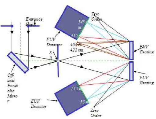
4.2.4 Optical layout . . . 61
4.2.5 Photometric assessment and spectral resolution . . . 69
4.3 Theoretical Results . . . 73
4.3.1 Radiometric modelling of star spectra . . . 73
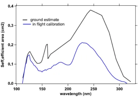
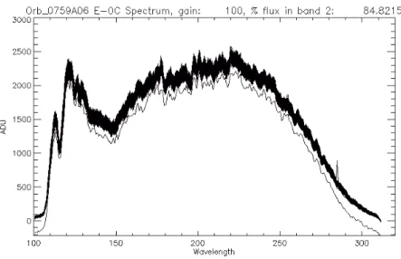
4.3.2 In-flight calibrations of stars . . . 74
5 Modelling Mercury’s hydrogen exosphere 77
5.1 Introduction . . . 77
5.2 SECTION I: The physics behind . . . 85
5.2.1 Definitions and basic exospheric theory . . . 85
5.2.2 Mechanisms of ejection from the surface: Maxwell-Boltzmann distributions . . . 86
5.2.3 Temperature mapping . . . 88
5.2.4 Ballistic motion of particles in the exosphere and external conditions 89 5.2.5 Sources of hydrogen at Mercury: Thermal processes . . . 91
5.2.6 Sinks of hydrogen at Mercury: Ionisation . . . 99
5.2.7 Deriving emission line brightness: radiative transfer and optical thickness (with Jean-Yves Chaufray) . . . 100
5.3 SECTION II: Monte Carlo model . . . 103
5.3.1 Coordinate system . . . 103
5.3.2 Flow of program . . . 103
5.3.3 Time evolution of the particle . . . 108
5.3.4 Euler solution to ballistic motion . . . 109
5.3.5 Outputs . . . 113 5.4 Validation . . . 114 5.4.1 Convergence criteria . . . 114 5.4.2 Chamberlain . . . 114 5.4.3 Thermalisation at surface . . . 120 5.5 Sensitivity study . . . 121
5.5.1 MB and MBF Velocity distribution functions . . . 122
5.5.2 Accommodation coefficient . . . 129
5.5.3 Source regions . . . 129
5.5.4 Comparison to Mariner 10 data . . . 132
5.5.5 Prediction of expected PHEBUS signal . . . 139
5.6 Summary . . . 142
6 Conclusion 145
Appendices 147
A SPICAM star table of 39 stars with flux above 800 R at 164 nm 147
B PHEBUS radiometric simulation brightness of emission lines 149
C SPICAV star table of 183 stars with flux above 60 R at 164 nm 157
D Short-term variations of Mercury’s sodium Na exosphere observed with very high spectral resolution 163
Chapter 1
Introduction
”For us who seek the truth without pre-conceived ideas, and without having a theory to support, it seems to us that the principle of matter remains as much unknown as the principle of force, the visible universe not being at all what it appears to our senses. ”
The planet Mercury is the first planet from the Sun, situated around one third of the distance between the Sun and the Earth, making it a privileged witness of solar-planetary interactions.
It also occupies a unique niche in the Solar System with its huge ground temperature amplitudes spanning hundreds of degrees (from 100 K to 600 K) as it faces the scorching whims of the Sun, with its weak but appreciable magnetic field for such a small body, and its tenuous exosphere bounded to the surface, made mostly of neutral atoms.
In this respect the Mercurian environment is a marvelous in-situ laboratory for complex plasma physics, involving dust, neutral-ion particle interactions and acceleration processes. Different tools can be used to study Mercury as a planet and probe its vicinity:
• Remote sensing: ground-based observatories such as the solar telescope THEMIS (Tenerife)
• In-situ observations: past missions such as Mariner 10, current space missions such as MESSENGER
• Models or physical simulations of the 3D neutral/ion environment, including Monte Carlo simulations of the ballistic motion of a great number of particles
All three tools working in synergy are necessary to gain the most detailed understanding: observations show which species and mechanisms are present, while models try to explain them with state-of-the-art physical approaches. In turn, models can predict many observables that can be compared with new (or old) observations.
It is not surprising that since the advent of modern techniques (spectroscopy, radars, high-resolution imagers), Mercury has been unveiling more and more of its hidden characteristics, despite the fact that after more than 50 years of investigations, it remains one of the least known planetary bodies in the Solar System. For instance, the very
location of Mercury close to the Sun and the difficulty to observe it directly has impeded a more systematic examination from ground-based observatories. Only since the 1980s have they become sufficiently sensitive and adapted to the study of Mercury’s exosphere. This developmental state of flow in science history, described by the philosopher of science Thomas S. Kuhn, is what Mercury science has been experiencing for the last 50 years, with many outstanding discoveries and new theories that have to be tested against measurements and coming from many different science groups. These theories will eventually lead to a paradigm, characterised by scientific consensus, thanks to the science outputs of current and incoming efforts such as the ESA/JAXA BepiColombo mission.
One of the main science problematics in today’s Mercury science concerns the formation, sustaining and evolution of the tenuous atmosphere of the planet, called the exosphere, as the planet is not large enough to retain by gravity a permanent thick atmosphere. From Mariner 10 in the 1970s, MESSENGER since 2008 and ground-based observations, the species that have been detected include H, He, O, Na, K, Ca and Mg.
Generally speaking, an exosphere is the uppermost layer of the atmosphere of a planet, where the particle density is so low that the particles no longer collide with each other and some are moving fast enough to reach the escape velocity and escape to space. In the case of Mercury, the exosphere starts at the surface, which gives rise to many original and peculiar processes, which can be classified into two categories:
• release from the surface: thermal, photon/electron desorption, meteoroid impact, solar wind sputtering
• depletion: Jeans escape, photoionisation, charge exchange or solar radiation pressure
These processes depend on the location of the particle on the planet, whether it is on the cool 100-K nightside or the hot 600-K dayside.
Hydrogen
One of the first species discovered in the exosphere of Mercury was atomic hydrogen H, through its characteristic emission at 121.6 nm, called Lyman-α. Since its discovery very few studies have been performed and even less observations are available. Analogy with the Moon has been used with much success and has managed to constrain the mechanisms at the origin of the release and loss of hydrogen around Mercury, namely (1) thermal desorption, (2) Jeans escape, (3) photoionisation and (4) solar radiation pressure. The reason hydrogen is interesting is that not only is it one of the fourth most abundant species on Mercury, although not the most bright, but it is also an ”end-member”; it is the species that is most extreme in every way because of its very low mass and its high velocity mobility in the exosphere. Using comparisons with the Moon it is also obvious that despite the similarities between the Moon and Mercury hydrogen does not react the same way on both these planets.
Also, despite being one of the first species detected on Mercury by Mariner 10, together with helium, no real attempts to model hydrogen have been done so far. In the tenuous exosphere of Mercury, all species are important for a complete understanding of its mechanisms. Hydrogen is no exception.
Introduction
1.0.1
Layout of thesis
This thesis deals with two aspects of hydrogen at Mercury, observational and theoretical, with the preparation of the UV spectrometer PHEBUS on board BepiColombo and the modelling of the neutral hydrogen exosphere.
Chapter 2 is intended to be an overview of Mercury’s science through history, browsing through its orbital characteristics and discussing the main scientific areas of investigation: surface, magnetosphere and magnetic environment, exosphere. A specific focus is put on recent exospheric studies, both observational and theoretical, dealing with other species than hydrogen. This chapter presents the background science necessary for the next chapters and briefly discusses the science objectives of the Mariner 10, MESSENGER and BepiColombo missions, as well as the use of the solar telescope THEMIS (situated in Tenerife) for observing the exosphere of Mercury.
Chapter 3 is aimed at setting up an in-flight calibration procedure for PHEBUS, based on that of the SPICAM/SPICAV UV spectrometers on board ESA Mars Express and Venus Express. As PHEBUS primary design is based on SPICAM/SPICAV, star calibration is performed from two stars chosen in the SPICAV star catalogue and tested for assessing the sensitivity of PHEBUS and the plausibility of in-flight/in-orbit calibrations. The list of stars, their spectral type and fluxes are presented at the end of the chapter.
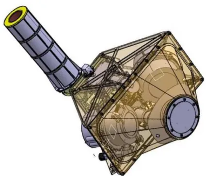
Chapter 4 introduces the UV spectrometer PHEBUS (Probing of Hermean Exosphere By Ultraviolet Spectroscopy) on board BepiColombo, and the radiometric modelling which is used to predict the expected science performance of the instrument, developed in close collaboration by N. Rouanet. A list of emissions and their brightness is provided, which proves that PHEBUS with both high spectral resolution and high sensitivity will be able to measure all the existing exospheric emissions and more, including hydrogen for which the wavelength range of the instrument has especially been chosen.
Chapter 5 presents the theoretical follow-up of the PHEBUS in-flight calibration. This chapter is a detailed description of the model SPERO for hydrogen neutral atoms that was developed in the last part of this thesis. SPERO (Simulation and Parsing of Exospheric neutRal atOms) is a full 3-D Monte Carlo numerical model that calculates the ballistic orbits of hydrogen particles released from the surface of Mercury up until 8 Mercury radii. After an historical report of previous studies on hydrogen, the classical theory of exospheres is discussed and presented. All theoretical release and loss processes are also discussed in the case of atomic hydrogen. The development of the Monte Carlo model, with the different algorithms and assumptions concerning the distribution function of the ejecta, is also thoroughly described, while a sensitivity study of all known parameters is presented.
Finally, thanks to the use of radiative transfer model of J.-Y. Chaufray (LMD), key notions are deducted and a comparison to the Mariner 10 original hydrogen Lyman-α data is possible and shown. Preliminary results concerning the dusk-dawn asymmetry and predictions are also highlighted which could be confirmed either by data from the ongoing MESSENGER mission (MASCS) or the future BepiColombo mission to Mercury. An application to PHEBUS is also shown, with hydrogen emissions applied to the instrument function giving the possible count rates of the EUV detector.
THEMIS observation
In the scope of studying the exosphere of Mercury, an observation campaign dedicated to the sodium exosphere, was carried out at the THEMIS observatory in Tenerife. This work lead to the publication in Geophysical Research Letters of an article entitled ”Short-term variations of Mercury’s sodium Na exosphere observed with very high spectral resolution”, which can be found in Appendix D.
In this manuscript, the subsolar point designates the point on the surface of the planet facing the Sun at zenith, thus on the dayside of the planet. To mirror this expression the opposite point on the surface of the Sun and directly facing the interplanetary space on the nightside of the planet is then referred to as the antisolar. However at some instances I do refer to this point as subspace, since it was a term that somehow fitted the description very well.
Chapter 2
Mercury: History and
context
”From this it results that the histories of all the worlds are traveling through space without disappearing altogether, and that all the events of the past are present and live forever in the bosom of the Infinite.”
2.1
The Planet Mercury
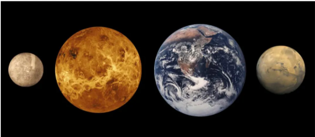
Mercury is the small, rocky planet located closest to the Sun in the solar system and the smallest of the terrestrial planets, Figure 2.1. Its main physical characteristics are summarised in Table 2.1 and compared to those of the Moon and Earth. In appearance Mercury resembles the Moon by its size, its cratered surface, the lack of satellites1 and
the absence of a substantial atmosphere, see Figure 2.2.
2.1.1
Orbital parameters
Mercury is in many ways the most extreme of all planets. Its orbit is the most eccentric with a value of 0.21 making it have a large variety in distances from the Sun, from 46 ×106
km at aphelion to 70 × 106 km at perihelion. This causes the solar flux received by the
planet to change by more than a factor of two throughout a Mercurian year.
The orbital tilt to the ecliptic is 7 degrees, making it possible to see transits of Mercury across the Sun only 13 to 14 times per century from Earth. The last observed transit occurred on 08 November 2006, see Figure 2.3, while the next one will take place on 09 May 2016.
1Although it is not common that satellites have satellites due to the instabilities they
might infer, it is not impossible. For example, there is proof that the satellite Rhea has had shepherd moons in the past (Jones et al., 2008).
Physical parameters
Mercury
Moon
Earth
Mean radius (km)
2439.7
1737.1
6371.0
Mass (kg)
3.30 · 10
237.35 · 10
225.97 · 10
24Mean density (g cm
−3)
5.43
3.34
5.51
Equat. surf. gravity (m s
−2)
3.70 (0.38 g)
1.62 (0.16 g)
9.81 (1 g)
Escape velocity (km s
−1)
4.25
2.38
11.18
Obliquity/axial tilt (
◦)
0.02
6.68
23.44
Sidereal rot. period (days)
58.6
27.3
1
Rotation velocity (m s
−1)
3.02
4.63
465.1
Albedo
a0.142
0.136
0.367
Aphelion (AU)
b0.47
−
1.02
Perihelion (AU)
b0.31
−
0.98
Eccentricity
0.21
0.05
0.02
Orbital period (days)
87.97
27.32
365.27
Orbital speed (km s
−1)
47.87
1.02
29.78
Inclination to ecliptic (
◦)
7.00
5.41
0
Main atmospheric constit.
Na,H
2,He
Ne,He,Ar
N
2,O
2trace
H,K,Ca,Mg,O
CH
4,CO
2O,Ar,H,He
Pressure at surface (nPa)
∼ 1.0
0.1
1013 · 10
11Max. surface temp. (K)
700
390
279
Min. surface temp. (K)
100
100
Altitude of exobase (km)
∼ 0
∼ 0
∼ 500
Magn. field, equator (nT)
230 − 290
none
50000
Magn. field tilt (
◦)
5 − 12
−
11.5
Satellite
none
−
Moon
Table 2.1: Mercury planetary data compared to that of the Moon and Earth. The most recent measurements (MESSENGER) were chosen when available, especially for the B-field values. The composition of Mercury’s exosphere is not well constrained and was measured by Mariner 10, MESSENGER and ground-based facilities to be He, H, O, Na, K, Ca and Mg. a The albedo, ranging between 0 and 1, is the ratio of the total
brightness backscattered by the surface of a planetary body to that of a perfect reflector (A = 1). b 1 AU = 1.496 · 106
Mercury: History and context
Figure 2.1: Size comparison of the terrestrial planets. From left to right: Mercury, Venus, Earth and Mars(Image NASA/ESA).
Due to its elliptic orbit, it is from Earth only possible to see Mercury, by the naked eye, in morning or evening when the Sun has not yet risen or when the Sun has just gone down the horizon. Mercury, with a maximum apparent diameter of only 13”, is a very bright object in the sky, and has a magnitude that varies from −2.6 to +5.7 depending on its orbital location. Because of its close proximity to the Sun (it never strays more than 28◦
away from the Sun), it is usually lost in the strong background sunlight.
Mercury’s period around the Sun is 88 days, and speeds through space at nearly 50 km per second, faster than any other planet. Its axial tilt is almost zero, 0.027 degrees, which is much smaller than even Jupiter at 3.1 degrees, preventing the planet from displaying its poles to the Sun and leaving them always in relative shadow.
In 1965 Pettengill and Dyce (1965) discovered from radar Doppler observations that the rotation of Mercury was not synchronously locked as had been believed for many years and equaled ∼ 58 days instead of 88 days. Mercury has a very slow rotation period that is exactly half of its synodic period making for a very peculiar counting of days and years; a single day (solar day) lasts exactly two Mercury years (sidereal). This is thought to be due to the eccentricity of Mercury’s orbit in combination with the gravitational influence from the Sun and other planets in the solar system, creating a 3:2 spin-orbit resonance, as shown in Figure 2.4.
Correia and Laskar (2004, 2010) have shown that as the orbital eccentricity of Mercury varied chaotically from near zero to more than 0.45 in the last 4×10⁹years and adding the viscous friction at the core-mantle boundary, the capture probability in a 3:2 resonance increases and can be favoured.
Mercury’s advance of perihelion amounts to 43 arcseconds per century with respect to classical Newtonian mechanics, an anomalous rate discovered first by Urbain Le Verrier in 1859 and ascribed to possible planetary bodies inside Mercury’s orbit (often nicknamed ”Vulcan”). This served historically as a test of the validity of Einstein’s General Theory of Relativity in 1916 and played a major role in the adoption of the then young theory.
Figure 2.2: The Moon seen from Earth (left) and Mercury imaged in true colours by the Wide Angle Camera (WAC) of the Mercury Dual Imaging System (MDIS) on board NASA MESSENGER in 2009 (right). The enhanced-colour view of Mercury on the right shows surface features not unlike the Moon’s. (Image Thierry Legault, NASA/Johns Hopkins University Applied Physics Laboratory/Carnegie Institution of Washington).
2.1.2
Internal structure, the magnetic field and
magneto-sphere
Models predict that the core of Mercury is very large (42% in volume) (see Fig. 2.5) and consists of mostly metallic (70%) and silicate (30%) materials, making it one of the densest planets in the solar system (5.43 g cm−3), only topped by Earth (5.51 g cm−3).
While the Moon completely lacks a magnetic field, Mercury possesses a very large liquid iron core sustained by tidal effects and generating through a dynamo effect a weak but stable dipolar magnetic field, probably fueled by the cooling of the core and the contraction of the entire planet after the ”late heavy bombardment” period, between 4.1 and 3.8 billion years ago (Breuer et al., 2007; Glassmeier et al., 2007).
The intensity of the magnetic field reaches around 300 nT at the equator, which is about 1.1% the corresponding value of Earth’s. Following the recent measurements of the MESSENGER probe, the magnetic field poles were found to be tilted between 5 and 12◦from the spin axis of the planet (Anderson et al., 2008).
The stable magnetic field is strong enough to make an obstacle to the solar wind creating a magnetospheric cavity probed by Mariner 10 and more recently by MESSENGER (Fig. 2.5). The magnetosphere traps solar wind ions and electrons that participate to the space weathering of the surface.
During its first flyby on 14 January 2008 followed by a second flyby on 06 October 2008, NASA MESSENGER showed that Mercurys magnetic field can be extremely dynamic (Slavin et al., 2008, Fujimoto et al., 2007) with the discovery of recurrent flux transfer
Mercury: History and context
Figure 2.3: Transit of Mercury on 8 November 2006 captured by the Solar Optical Telescope on board the Japanese solar satellite SOLAR-B/Hinode, just after it crossed the solar limb(Image JAXA/NASA/PPARC).
events being a signature of magnetic reconnection between the solar wind frozen-in field and the planet’s own magnetic field (Slavin et al., 2009; Slavin et al., 2009).
MESSENGER’s third flyby on 29 September 2009 showed that the solar wind plasma can then be allowed to enter the magnetosphere in bursts lasting 2 to 3 minutes and at a uniquely high rate owing to the proximity of Mercury to the Sun (Slavin et al., 2010). Following this new picture, two sources are thought to contribute to the existence of a magnetospheric plasma: the solar wind (through reconnection or direct entry along open field lines), but also pick-up ions created by UV photoionisation and electron impact ionisation of the neutral exosphere and subsequently driven along magnetic field lines (Slavin et al., 2008).
Accelerated by intense electric fields in the magnetotail, the magnetospheric plasma can in turn impact the surface of the planet and release volatiles (Orsini et al., 2007). In doing so, it contributes as an additional source to the formation of the neutral exosphere. Charged particle acceleration mechanisms occurring at Mercury are now under close investigation by MESSENGER (Zelenyi et al., 2007). The study of the magnetosphere of Mercury, its energy content and dynamics is only starting.
2.1.3
Surface
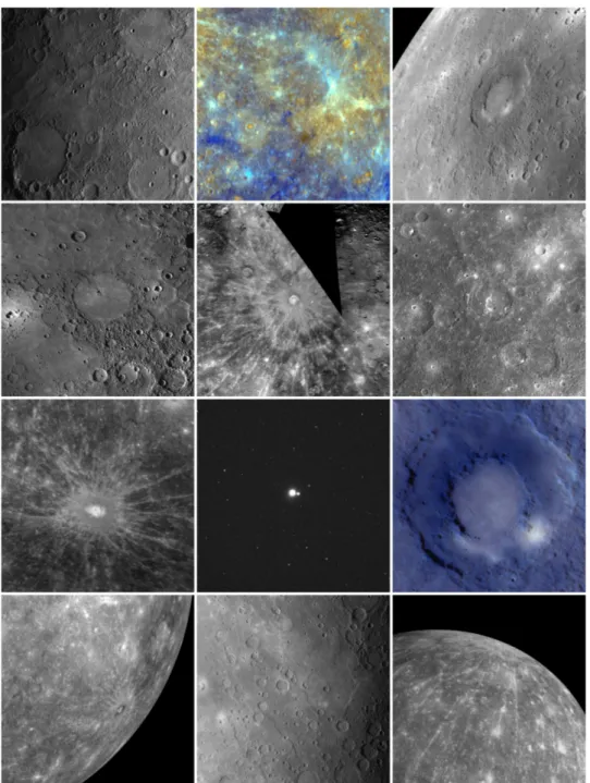
Morphologically speaking, Mercury shows an astonishing similarity to the Moon (see Figure 2.2) with its mare-like plains, montes, planitiae, rupes and valles, and heavy cratering (Figure 2.6), proving that it has been partly geologically inactive for billions of years.
Figure 2.4: The 3:2 spin-orbit resonance of Mercury. a The planet presents the same face to the Sun every two passages at pericenter. b Dynamical stability of the resonant orbit: the Sun’s position is shown in a reference frame centered on Mercury and rotating with the solid body of the planet. The angle between the pericenter axis and the long axis of the planet oscillates like a pendulum. (Image Dermott (2004))
Strom et al. (2008) concluded from new observations of the cratering record during the first flyby of MESSENGER that the plains formed no earlier than 3.8 billion years ago while lower densities of craters on certain basins (like Raditladi) may be younger than 1 billion year. The curious feature of high ridges in Mercury’s surface is believed to be due to the cooling of the core and mantle and their subsequent shrinking, when the surface had already solidified (Solomon et al., 2008).
The discovery of volcanic evidence at Mercury was one of the main highlights of the first MESSENGER flyby (Head et al., 2008) and is thought to explain the formation of plains on Mercury. By comparison with the Moon, high resolution images (150 m) showed deformation vents of pyroclastic origin around the Caloris basin (the youngest known large basin) which were significantly different from the lunar impact basins known properties (albedo, geomorphological structure) (Murchie et al., 2008).
New images and data from the second and third flybys suggested that the role of volcanism was predominant in explaining these formations, while volcanic activity might have spanned previously unsuspected long periods, from the planet’s formation to well into the second half of its history (Prockter et al., 2010).
2.1.4
Exosphere
Mercury, with an equatorial radius of 2440 km, is the smallest planet in the solar system but is also too small to retain a thick atmosphere. However, Mariner 10, ground-based instruments and now MESSENGER have shown that a tenuous surface-bound exosphere exists, where barely any collisions between constituents occur. It is mainly composed of (see Hunten et al., 1988; Killen et al., 2007, Table 2.1):
• Light species such as hydrogen (H and H2)
Mercury: History and context
Figure 2.5: Mercury’s space environment and surface features (Image ESA/BepiColombo)
• Alkali species such as sodium Na, potassium K, calcium Ca and magnesium Mg. • Heavier species such as oxygen O, with expected traces of molecular oxygen O2,
nitrogen N2 and carbon dioxide CO2
The relative abundances of these species are badly constrained and need further investigation from current and upcoming space missions (Killen et al., 2007). It is also believed that Mercury has traces of water ice H2O located in the eternally dark polar
regions. Species such as C, CO, CO2, N2 and Li have been suggested (Sprague et al.,
1996; Hunten et al., 1988) but were never detected, while hypothetical OH or S species were suggested to account for bright deposits at the poles.
According to models and observations (see for instance Leblanc and Johnson, 2003), the neutral species originate from the surface of Mercury and are released in the atmosphere by a number of processes that will be detailed in Chapter 2. They can be classified into three categories:
• Photon- and low energy electron-induced mechanisms (photon-stimulated desorp-tion, electron-stimulated desorption) due to electronic excitation of a surface atom • Sputtering effects due to impact (solar wind, magnetospheric ions, meteorites) • Thermal vaporization of atoms (hydrogen and alkali atoms mostly) due to the high
surface temperature of Mercury
Typical dayside densities at the surface range between 100 and 4×104cm−3while strong
nightside variations are seen (Hunten et al., 1988). For instance, as shown in Table 2.2, hot (475 K) and cold (100 K) populations have been observed for hydrogen H, interpreted
Figure 2.6: The surface of Mercury as seen by MESSENGER. Geddes Crater, smooth plains, young volcanism and the rays of Hokusai.
(Image NASA/Johns Hopkins University Applied Physics Laboratory/Carnegie Institution of Washington)
Mercury: History and context
Species
Densities
aColumn abundance
bTemperature
c(10
7cm
−3)
(10
13cm
−2)
(K)
expected/measured
measured
measured
H
∼ 0.02
0.005
110
(night), 420 (day)He
2.6
2.0
575
Na
11
0.02
750 − 1200
K
14
1.0 × 10
−4O
4.2
0.7
Ca
−
1.0 × 10
−6Table 2.2: Upper limit of number densities and column abundances at Mercury inferred from Mariner 10 occultation experiment (Broadfoot et al., 1976 and Hunten et al., 1988). Large variations reported by Milillo et al. (2005) and references therein are expected. Temperatures derived from scale heights are also mentioned for a few species. a see Hunten et al.
(1988),b see Strom and Sprague (2003),c see Milillo et al. (2005).
as a dayside and a nightside component (see Milillo et al., 2005) The column density of observed constituents has an upper limit of 1012cm−2 (Killen and Ip, 1999).
During the different flybys of Mariner 10 in 1974 (Shemansky and Broadfoot, 1977) and more recently by MESSENGER (discovery of Mg by McClintock et al., 2009) as well as ground-based observations (discovery of Na and K by Potter and Morgan, 1985, 1986, and of Ca by Bida et al., 2000), the exospheric emissions arising from the excitation (resonant or not) of neutral species were observed and can serve to get an estimate of exospheric neutral densities.
Vervack et al. (2010) performed observations with the spectrometer on board MES-SENGER of Na, Ca and Mg atoms with evidence of Ca+ ions extending far back
in the magnetotail. The neutral species exhibited very different distributions (for instance, sodium Na displayed a two-temperature distribution, while the weak Mg emission appeared to be nearly uniformly distributed) which indicated that multiple processes might drive the formation of these exospheric species.
2.2
History and science: Ancient
Surprisingly old records of Mercury have been discovered. The Mul.Apin tablets, dating back to 500 BC account for observations describing the risings and settings of stars believed to have been made by Babylonian astronomers around 1000 BC. The tablets, containing the earliest and most comprehensive surviving star catalogue from Mesopotamia, refer to Mercury as Ninurta, a planet who ”rises or sets in the east or in the west within a month” (Hobson, 2009).
The Greeks knew around 450 BC that there were five planets, called Astra Planeta −the wandering stars−, and named them Phainon (Saturn), Phaethon (Jupiter), Pyroeis (Mars), Eosphoros (Venus), and Stilbon (Mercury). Believing Mercury to be two planets they named it Stilbon/Apollo in the morning and Hermeaon/Hermes in the evening. However around the 4th century BC they came to realise that it was two aspects of the same planet, naming it as the messenger of the gods, Hermes. The Romans later named the planet ’Mercury’, in reference to the Greek God Hermes in their mythology.
Figure 2.7: Skull owl (left) and Shooting owl (right), aspects of Mercury by the Mayans, as depicted in the Popol Vuh(Image Tedlock, 1985).
Cicero, the famous Roman rhetorician of the first century BC, mentioned Mercury in his De Natura Deorum:
Below this [the orbits of Saturn, Jupiter and Mars] in turn is the Stella of Mercurius, called by the Greeks Stilbon (the gleaming), which completes the circuit of the zodiac in about the period of a year, and is never distant from the sun more than the space of a single sign, though it sometimes precedes the sun and sometimes follows it.
Cicero, De Natura Deorum, 45 BC. In Southern America, the Mayas charted the motion of the visible planets including Mercury. Records of their detailed observations are found in the Dresden Codex, a Mayan book from 1000 AD, that is deemed to be a copy of an earlier text at least 300 years older. The astonishingly accurate text describes Mercury’s visibility, location in the sky and a description of conjunctions with other planets at specific dates. The Mayans also calculated that Mercury would rise and set in the same place in the sky every 2200 days. The Mayan had the notion of Mercury as the messenger of the gods of the underworld Xibalba, represented by four owls, two for the waxing/waning morning star aspect and two for the waxing/waning evening star aspect (Tedlock, 1985). Skull owl and Shooting owl, two of these aspects, can be seen in Figure 2.7.
Around 100 AD the Roman-Egyptian astronomer Ptolemy described a complex system of circles to describe the motion of the planets, based on a geocentric world view. In this system, Earth was in the middle instead of the Sun, and then Mercury went in a circular orbit around it, moving in a epicycle, see Figure 2.8. Later, in his large treatise Almagest, Ptolemy correctly suggested that no transits of planets, such as Mercury, across the face of the Sun had been observed either because it was too small to see, or because the transits were too infrequent.
1200 years after Ptolemy, Ibn al-Shatir (1304−1375), an Arab astronomer, mathematician and inventor from Syria, wrote an astronomical treatise The Final Quest Concerning
Mercury: History and context
Figure 2.8: Ptolemaic system of the inner planets. The Earth is in the middle, while Mercury, Venus and the Sun all follow epicycles around it.
Figure 2.9: Ibn al-Shatir’s drawing circa 1350 showing his reformation of the Ptolemaic system, predicting the motion of Mercury around the Sun
the Rectification of Principles, see Saliva (1987), in which he drastically reformed the Ptolemaic model by introducing extra epicycles, subsequently eliminating the Ptolemaic equant and eccentrics, for an example applied to Mercury’s orbit see Figure 2.9. This reform was one of the major ones that led to the evolution of the heliocentric system that, curiously enough, left Mercury in exactly the same orbit as in the Ptolemaic system, only revolving around the Sun this time instead of the Earth.
2.3
Science: In modern times
2.3.1
Early Optical observations
Even though Mercury,is a very bright object in the sky whith magnitude varying from −2.6 to +5.7 depending on its orbital location, it is very hard to observe the planet from Earth because of its close proximity to the Sun and because of its eccentric orbit. Therefore it is only possible to see it, by eye, in morning or evening when the Sun has not yet risen or when the Sun has just gone down the horizon.
The difficulty in observing Mercury from the ground has led to it being the planet least studied, with most erroneously attributed features that have later been disproved. The first known observation using a telescope was made by Galileo early in the 17th century but his telescope was not powerful enough to observe any phases.
In 1631 Pierre Gassendi observed the transit of Mercury on the Sun, as predicted two years before by Johannes Kepler (from his newly completed Rudolphine tables): he used a telescope to project an image 20 cm in diameter of the sun upon a white screen (see Gassendi and the Transit of Mercury, Nature, 128, 3236, 787, 1931).
Using a telescope only slightly more powerful than Galileo, Giovanni Battista Zupi (Zupus) discovered in 1639 that Mercury had phases just like the Moon and Venus, a potent evidence that Mercury was orbiting the Sun and giving strength to the argumentation of heliocentric theories, Figure 2.10. This was later observed independently by Johannes Hevelius in 1644 who also observed a transit in 1661 (Hevelius, 1662), see Figure 2.11. The very rare occultation of Mercury by Venus in 1737 was recorded by John Bevis. The next one is expected to take place in 2133.
By the turn of the 19th century, with the increasing size of reflecting telescopes, several
scientists, like Johann Schr¨oter and his assistant Karl Harding in Germany, Giovanni
Schiaparelli in Italy, had described some surface features of Mercury, Figure 2.12. Schr¨oter
claimed that due to irregularities in brightness, mountain ranges existed on Mercury,
among which one towered at 18 km (Schr¨oter, 1800). Both Schr¨oter and Bessel (1813)
incorrectly derived a period of 24 hours with a rotation axis at 70◦
to the orbital plane. At the end of the same century, Schiaparelli estimated a new, though incorrect, value of 88 days for the period (Schiaparelli, 1891), which was not corrected until the advent of radar observations in 1965. By his own words:
Among the planets known by the ancients, none is so difficult to observe as Mercury and none presents as many difficulties for the study of its orbit as well as its physical nature. Being impossible to observe during the night, and rarely possible during twilight, there is no other solution than studying it in full daylight, in the presence of the Sun always in the vicinity, and through an illuminated atmosphere.
Mercury: History and context
Figure 2.10: Mercury’s phases seen from Earth(Image adapted from NMS University).
Figure 2.11: Part of Hevelius’ report of the transit of Mercury across the Sun with the corresponding phases(Image Hevelius (1662)).
Figure 2.12: Map of Mercury drawn by G. Schiaparelli in 1889 (left) and by Antoniadi in 1934 (right)(Image Antoniadi (1934)).
Concerning the mapping of Mercury, the Greek astronomer Eugene Antoniadi published in 1934 a book in French containing both maps and observations, mostly based on Schiaparelli’s works from the 1880s and on Mercury’s supposed Sun-synchronous rotation (Antoniadi, 1934). A very interesting historical account of Mercury’s optical cartography efforts can be found in McEwen (1935), Dollfus (1953), who resolved features down to 300 km, and more recently in the amateur astronomer’s paper of Frassati et al. (2002). From 1841 to 1859, the French astronomer Urbain Le Verrier, encouraged by his successful prediction of the presence of Neptune using celestial mechanics, observed an anomalous rate of precession of Mercurys orbit around the Sun that could not be completely explained by Newtonian mechanics and perturbations by the known planets (Le Verrier, 1859). Le Verrier analysed available timed observations of transits of Mercury over the Sun’s disk from 1697 to 1848 and showed that the measured precession rate disagreed with Newton’s theory by an amount initially estimated as 38” (arc seconds) per century and later re-calculated at 43”.
As an analogy with the analysis of the motion of Uranus that led to the discovery of Neptune as a perturbing body, Le Verrier proposed that the motion of Mercury was perturbed by a hypothetical planet or group of corpuscules orbiting inside Mercury’s orbit and soon baptized Vulcan. General Relativity developed by Albert Einstein in the 1910s gave an explanation to the observed advance of perihelion in terms of space-time curvature.
In 400 years, Mercury, this little wandering rock which might look insignificant, had helped to install two major new theories at the time: heliocentrism and general relativity.
Mercury: History and context
2.3.2
Modern ground-based observations
Use of radar techniques
The first modern radio observation was in 1962 when Soviet scientists under V. Kotelnikov in Crimea managed to reflect not less than 53 radar signals off the surface of Mercury. Three years later, using the newly built incoherent scatter radar of Arecibo (Puerto-Rico), Pettengill and Dyce (1965) showed that its rotational period was 59 ± 5 days completely overturning all that had been believed for the past 150 years. As any change of scientific paradigm, the implications were fascinating, indicating that ”either the planet has not been in its present orbit for the full period of geological time or that the tidal forces acting to slow the initial rotation have not been correctly treated previously” (Pettengill and Dyce, 1965).
Between 1960 and 1961, it was also confirmed by analysis of the planetary radio wave emission between 3.45 and 3.75 cm wavelength with the 25.9 m reflector of Michigan University that Mercury’s nightside was warmer than commonly assumed (Howard, 1962), questioning the accepted idea of the 1:1 ratio orbit, as this would have left the planet much colder on the nightside.
Dyce, Pettengill and Shapiro (1967) from the Smithsonian Astrophysical Observatory (SAO) were working on the interpretation of the new puzzling radar data, when Giuseppe ’Bepi’ Colombo (1920 − 1984), an Italian astronomer who was a visiting scientist of SAO, hypothesised that Mercury could be in a 3:2 resonance (Colombo, 1965). As a main collaborator of Colombo (Colombo and Shapiro, 1966), Shapiro recalls:
Colombo realized almost immediately that 58.65 days was exactly two-thirds of 88 days. Mercury probably was locked into a spin such that it went around on its axis one-and-a-half times for every once around the planet. The same face did not always face the Sun. That meant that [...] the orbital motion and spin rotation of Mercury were very closely balanced, so that Mercury almost presented the same face to the Sun during this period.
Irwin Shapiro, quoting Giuseppe Colombo, in Butrica (1996). The 3:2 resonance was later confirmed at the arrival of the American mission Mariner 10 in 1974 and explained why observers had always managed to see only one side of Mercury since it is always showing the same side every second orbit, while all other sides would not be properly viewed due to poor viewing conditions. The formidable intuition of Colombo fostered many studies on the origin and consequences of the rotation of Mercury from Liu and O’Keefe (1965) to Correia and Laskar (2010).
The story of Colombo with Mercury did not stop there: he also suggested in 1970 how to put the Mariner 10 spacecraft into an orbit that would bring it back repeatedly to Mercury, using the gravitational slingshot maneuver provided by Venus to bend its original flight path and decelerate the spacecraft on its way to the inner solar system.
The advent of spectroscopy and polarimetry
As soon as 1932, attempts were made to detect an atmosphere at Mercury using either IR spectroscopy (Adams and Dunham, 1932, who failed to detect CO2) or polarimetry
(Lyot, 1929). The optical studies of Lyot paved the way to increase the resolution of the observations always pushing away the observational limits: in 1942, he managed to observe Mercury at an angular distance of 2◦
from the Sun using a 11-m long sunshade mounted on a bamboo stick (Dollfus, 1953). Lyot concluded from his early polarimetric attempts
(Lyot, 1930) that Mercury’s polarisation was almost identical to that of the Moon at a wavelength of 580 nm.
By using the polarisation of light, it is possible to detect an atmosphere around a planet or a natural satellite, since the scattering by molecules or aerosols may polarise the reflected light of the studied body. In the 1950s, Mercury was thought, because of its small size, to have lost its atmosphere due to atomic and molecular escape into space.
Performing polarisation measurements at the Pic du Midi Observatory in the French Pyr´en´ees, Audouin Dollfus (1924 − 2010) set an upper limit to the atmosphere, estimating the maximum molecular atmospheric pressure to be under 25 Pa (Dollfus, 1961, Dollfus and Auri`ere, 1974), the real value being around 1 nPa. Dollfus and Auri`ere (1974) also confirmed Lyot’s first results by showing that Mercury’s surface was made of the same pulverised basalt, or regolith, as the lunar samples that the Apollo missions had returned. In parallel to polarimetric measurements, IR spectroscopy were undertaken but failed to
detect any sign of molecules such as CO2, O2 or H2O (Spinrad et al., 1965; Poppen et
al., 1973) even though H and CO2 were reported by Kozyrev (1964) and Moroz (1964)
but never confirmed (Kellermann, 1966). Radiogenic40Ar seemed at the time the likeliest
species to be detected (Field, 1964). Mariner 10 later confirmed the absence of detectable molecules and infirmed the suggestion about the preeminence of Ar by setting stringent limits on the constituents with the UV spectrometer experiment (Kumar, 1976).
The discovery of sodium Na by resonance scattering of sunlight from sodium atoms (Potter and Morgan, 1985) launched a new era in the observation of Mercury’s exosphere. Potter and Morgan (1986) also detected potassium K using the McMath telescope at the Kitt Peak observatory and showed that the ratio of emission between sodium and potassium could reach anomalously large values of Na/K ∼ 80 − 100, larger than any other known body in the solar system (except comets).
Many studies have tentatively tried to explain this ratio with different datasets (Potter and Anderson, 2002; Killen et al., 2010), until Doressoundiram et al. (2010), using the NTT (ESO, Chile) and CFHT (Hawaii) 3.6-m telescopes, measured in high resolution spectroscopy Na/K ratios ranging between 80 and 400 depending on the position in
the exosphere. They reported also that potassium and sodium exospheres exhibited
very different spatial distributions, which could be at the origin of the anomalous rate. The sodium and potassium modelling approach of Leblanc and Doressoundiram (2011) corresponding to these observations pointed the global day/night transport, the loss rate and the desorption efficiencies as the main factors responsible for the spatial distribution of the observed ratios.
Another fascinating facet of the sodium exosphere is its high temporal and spatial variability, documented since the start of the alkalis observation era (Potter et al., 2006, Leblanc et al., 2009). Long-term observational surveys have given a good statistical sampling of annual (Potter et al., 2007) and diurnal cycles (Potter et al., 2006) of the sodium exosphere, which have been associated with the solar wind.
Reconnection between the interplanetary magnetic field lines and those of Mercury on the dayside magnetopause may favour the bursty entrance of solar wind plasma into the cusp, which in turn may impact the surface and trigger, via ion-sputtering, the refilling of the Na exosphere (Massetti et al., 2007). Exospheric temperatures inferred for sodium are of the order of 1000 K as in shown by Killen et al. (1999) using the echelle spectrograph of McDonald Observatory or more recently by Leblanc et al. (2009) using the Franco-Italian solar telescope THEMIS.
Mercury: History and context
Figure 2.13: The solar observatory THEMIS in Tenerife(Image M. Simon Wedlund).
THEMIS: a new window on Mercury
The solar telescope THEMIS (T´elescope H´eliographique pour l’´Etude du Magn´etisme et des Instabilit´es Solaires) is situated in Tenerife, Canary Islands, Figure 2.13). Its originality lies in its versatility and different modes ranging from high resolution spectrometry to spectropolarimetry, offering a unique perspective on Mercury’s exospheric emissions. Built in 1996, THEMIS is perfect to observe Mercury in close proximity to the Sun, even during daylight, since the telescope was originally built to observe the Sun directly. It consists of a 90-cm primary mirror with a focal length of 15.04 m (L´opez Ariste et al., 2000).
Several studies have been performed looking at the D1(589.6 nm) and D2(589.0 nm) lines
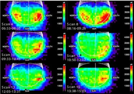
of Na (Leblanc et al., 2008, 2009) and characterising the spatial and temporal variations of brightness and Doppler shifts. Scans across the bright side of Mercury were made and reveal asymmetries between North and South hemispheres and the dynamics of these emissions, see Figure 2.14. Polarimetric measurements of D1 and D2 were successfully
carried out in 2010 (A. L´opez Ariste, personal communication), and could help characterise the weak magnetic field of Mercury as the polarisation/depolarisation is thought to be arising from the Hanle effect.
A description of the observatory and the observational modes of THEMIS is available here: http://www.themis.iac.es/.
Figure 2.14: Brightness of the Sodium emission during six consecutive scans performed with THEMIS (CNRS/CNR) on 13 July 2008. The disk of Mercury is highlighted in white(Image Leblanc et al. (2009)).
2.3.3
Missions
So far only two space missions have successfully been deployed and reached Mercury, Mariner 10 and MESSENGER. A third, BEPI-COLOMBO, is in its building stage and will be launched in 2014. Due to Mercury’s close proximity to the Sun, missions to Mercury have to take extra precautions to protect the instruments from the intense heat and radiation emitted from the star. To counteract these problems the spacecrafts have to be equipped with specially designed sunscreens and solar panels to keep the instruments in a safe working environment. Another problem is the difficult maneuver to make the spacecraft slow down and enter an orbit around Mercury due to the powerful gravitational field of the Sun that could easily accelerate the satellite and send it in a trajectory out of the solar system.
Mariner 10
In 1974-75 the first space probe reached Mercury.
Mariner 10, Figure 2.15 carried on board seven experiments to investigate Mercury: extreme ultraviolet spectroscopy, magnetometer, television imaging, infrared radiometry, plasma, charged particles, and radio wave propagation, see Figure 2.16.
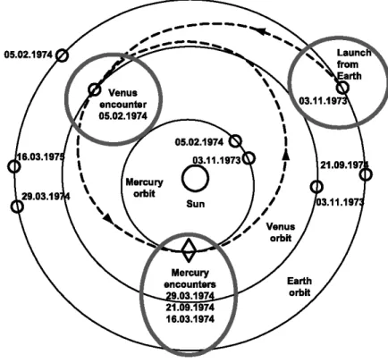
Mariner 10, a successful NASA collaboration was not only the first mission to Mercury but also the first mission ever to use gravitational assisting in order to reach it, the first mission to visit more than one planet at the same time and also the first to make multiple flybys of a planet (Mercury)In Figure 2.17 the complex trajectory of Mariner 10 can be seen.
Mercury: History and context
Figure 2.15: Artist view of Mariner 10 mission to Mercury(Image JPL)
Figure 2.16: Payload of Mariner 10 mission to Mercury(Image Dunne and Burgess (1978))
It also managed, for the first time ever, to take magnificent photographs of parts of the surface of Mercury. Unfortunately Mariner 10 was aligned such that it looked upon the same surface each time, leaving half the planet unexplored.
The main objective of Mariner 10 was to explore Mercury’s (and Venus) atmosphere, surface, environment and physical characteristics. Among the many discoveries was the Moon-like appearance of the surface that was revealed in the over 2800 photos taken. Another discovery was of the tenuous surface-bounded exosphere that separates it from the Moon together with the weak dipolar magnetic field.
Mariner 10 was a flyby mission, never meant to be inserted into orbit, and as such was limited in science to the three flybys performed. Because of this several features, such as the hydrogen exosphere, was never observed long enough to give conclusive data, despite this and several technical problems, it managed to greatly improve the existing knowledge of Mercury while at the same time raising a multitude of other questions.
MESSENGER
In 2004, 30 years after the Mariner 10 mission, the second mission to Mercury
was launched. Also a NASA mission, the MESSENGER (MErcury Surface, Space
ENvironment, GEochemistry and Ranging) probe has so far managed to make three flybys of Mercury, making a huge contribution to the understanding of Mercury. Among these, MESSENGER as depicted in Figure 2.19, has successfully managed to image the before unseen side of Mercury, completing the global map of the planet and made spectroscopic studies of the multitude of species in its exosphere, including for the first time Mg (McClintock et al., 2009).
Messengers main objective is to complete and complement the observations made by Mariner 10 and specifically to explore the nature of Mercury’s exosphere and magnetosphere, characterize the chemical composition of the surface, the geological history and the size and state of the core.
MESSENGER has an extensive payload of eight highly sensitive instruments. The instru-ments include the Mercury Dual Imaging System (MDIS), the Gamma-Ray and Neutron Spectrometer (GRNS), the X-Ray Spectrometer (XRS), the Magnetometer (MAG), the Mercury Laser Altimeter (MLA), the Mercury Atmospheric and Surface Composition Spectrometer (MASCS), and the Energetic Particle and Plasma Spectrometer (EPPS), Figure 2.20.
The MESSENGER, just as Mariner 10, uses gravity assisted trajectories to reach Mercury and in doing so has made, as of yet, both Earth, Venus and Mercury flybys. However, unlike Mariner 10 who only made flybys, the MESSENGER is expected to be inserted into orbit around Mercury in early spring 2011 after its third flyby.
BepiColombo
The scientific objectives of the ESA/JAXA mission to Mercury, BepiColombo, are very similar to those of NASA’s mission MESSENGER. This is due to historical collaboration between the missions to increase the scientific return of the instruments. BepiColombo is in the building stages for launch in 2014 on an Ariane 5 rocket and is composed of two orbiters, the Mercury Magnetospheric Orbiter (MMO) developed by JAXA and the Mercury Planetary Orbiter (MPO) developed by ESA.
The scientific payload of MPO consists of eleven instrument packages: the BepiColombo Laser Altimeter (BELA), the Mercury Radiometer and Thermal Infrared Spectrometer (MERTIS), the Ultra-Violet Spectrometer (PHEBUS), the Spectrometer and Imagers for
Mercury: History and context
Figure 2.17: Mariner 10’s gravity assisted trajectory past Venus on its way to Mercury (Image Balogh et al. (2007)).
Figure 2.18: Messengers gravity assisted trajectory to Mercury (Image Balogh (2007)).
Figure 2.19: Artist view of MESSENGER mission to Mercury (Image NASA)