HAL Id: hal-02110856
https://hal.archives-ouvertes.fr/hal-02110856
Submitted on 3 May 2019
HAL is a multi-disciplinary open access
archive for the deposit and dissemination of
sci-entific research documents, whether they are
pub-lished or not. The documents may come from
teaching and research institutions in France or
abroad, or from public or private research centers.
L’archive ouverte pluridisciplinaire HAL, est
destinée au dépôt et à la diffusion de documents
scientifiques de niveau recherche, publiés ou non,
émanant des établissements d’enseignement et de
recherche français ou étrangers, des laboratoires
publics ou privés.
Basic Properties of Star-forming Galaxies
Daichi Kashino, John Silverman, David Sanders, Jeyhan Kartaltepe,
Emanuele Daddi, Alvio Renzini, Giulia Rodighiero, Annagrazia Puglisi,
Francesco Valentino, Stéphanie Juneau, et al.
To cite this version:
Daichi Kashino, John Silverman, David Sanders, Jeyhan Kartaltepe, Emanuele Daddi, et al.. The
FMOS-COSMOS Survey of Star-forming Galaxies at z
∼ 1.6. VI. Redshift and Emission-line
Cat-alog and Basic Properties of Star-forming Galaxies. Astrophysical Journal Supplement, American
Astronomical Society, 2019, 241 (1), pp.10. �10.3847/1538-4365/ab06c4�. �hal-02110856�
THE FMOS-COSMOS SURVEY OF STAR-FORMING GALAXIES AT Z ∼ 1.6 VI: REDSHIFT AND EMISSION-LINE CATALOG AND BASIC PROPERTIES OF STAR-FORMING GALAXIES
Daichi Kashino,1 John D. Silverman,2 David Sanders,3Jeyhan Kartaltepe,4Emanuele Daddi,5 Alvio Renzini,6 Giulia Rodighiero,7 Annagrazia Puglisi,5Francesco Valentino,8 St´ephanie Juneau,9Nobuo Arimoto,10
Tohru Nagao,11 Olivier Ilbert,12 Olivier Le F`evre,12 and Anton. M. Koekemoer13
1Department of Physics, ETH Z¨urich, Wolfgang-Pauli-strasse 27, CH-8093, Z¨urich, Switzerland
2Kavli Institute for the Physics and Mathematics of the Universe, the University of Tokyo, Kashiwanoha, Kashiwa, Chiba 277-8583, Japan
(Kavli IPMU, WPI)
3Institute for Astronomy, University of Hawaii, 2680 Woodlawn Drive, Honolulu, HI 96822, USA
4School of Physics and Astronomy, Rochester Institute of Technology, 84 Lomb Memorial Drive, Rochester, NY 14623, USA 5Laboratoire AIM-Paris-Saclay, CEA/DSM-CNRS-Universit´e Paris Diderot, Irfu/Service d’Astrophysique, CEA-Saclay, Service
d’Astrophysique, F-91191 Gif-sur-Yvette, France
6INAF Osservatorio Astronomico di Padova, vicolo dell’Osservatorio 5, I-35122 Padova, Italy
7Dipartimento di Fisica e Astronomia, Universit´a di Padova, vicolo dell’Osservatorio, 2, I-35122 Padova, Italy
8Dark Cosmology Centre, Niels Bohr Institute, University of Copenhagen, Juliane Maries Vej 30, DK-2100 Copenhagen, Denmark 9National Optical Astronomy Observatory, 950 North Cherry Avenue, Tucson, AZ 85719, USA
10Astronomy Program, Department of Physics and Astronomy, Seoul National University, 599 Gwanak-ro, Gwanaku-gu, Seoul 151-742,
Korea
11Graduate School of Science and Engineering, Ehime University, 2-5 Bunkyo-cho, Matsuyama 790-8577, Japan
12Aix Marseille Universit´e, CNRS, LAM - Laboratoire d’Astrophysique de Marseille, 38 rue F. Joliot-Curie, F-13388 Marseille, France 13Space Telescope Science Institute, 3700 San Martin Drive, Baltimore, MD 21218, USA
ABSTRACT
We present a new data release from the Fiber Multi-Object Spectrograph (FMOS)-COSMOS survey, which contains the measurements of spectroscopic redshift and flux of rest-frame optical emission lines (Hα, [N ii], [S ii], Hβ, [O iii]) for 1931 galaxies out of a total of 5484 objects observed over the 1.7 deg2 COSMOS field. We obtained H-band and
J -band medium-resolution (R ∼ 3000) spectra with FMOS mounted on the Subaru telescope, which offers an in-fiber line flux sensitivity limit of ∼ 1 × 10⁻¹⁷ erg s−1 cm−2 for an on-source exposure time of five hours. The full sample contains the main population of star-forming galaxies at z ∼ 1.6 over the stellar mass range 109.5
. M∗/M . 1011.5,
as well as other subsamples of infrared-luminous galaxies detected by Spitzer and Herschel at the same and lower (z ∼ 0.9) redshifts and X-ray emitting galaxies detected by Chandra. This paper presents an overview of our spectral analyses, a description of the sample characteristics, and a summary of the basic properties of emission-line galaxies. We use the larger sample to re-define the stellar mass–star formation rate relation based on the dust-corrected Hα luminosity, and find that the individual galaxies are better fit with a parametrization including a bending feature at M∗≈ 1010.2 M , and that the intrinsic scatter increases with M∗ from 0.19 to 0.37 dex. We also confirm with higher
confidence that the massive (M∗& 1010.5 M ) galaxies are chemically mature as much as local galaxies with the same
stellar masses, and that the massive galaxies have lower [S ii]/Hα ratios for their [O iii]/Hβ, as compared to local galaxies, which is indicative of enhancement in ionization parameter.
Corresponding author: Daichi Kashino
Over the last decade, numerous rest-frame optical spectral data of galaxies at 1 . z . 3 have been deliv-ered by near-infrared spectrographs installed on 8–10-m class telescopes (e.g., Steidel et al. 2014; Kriek et al. 2015;Wisnioski et al. 2015;Harrison et al. 2016). These datasets have revolutionized our understanding of the formation and evolution of galaxies across the so-called ‘cosmic noon’ epoch that marks the peak and the subse-quent transition to the declining phase of the cosmic star formation history. Before the data flood by such large near-infrared surveys, however, the relatively narrow redshift range of 1.4 < z < 1.7 had long been dubbed the ‘redshift desert’ since all strong spectral features in the rest-frame optical such as Hα, [O iii], Hβ, and [O iii] are redshifted into the infrared, while strong rest-frame UV features such as C iv/S ii absorption lines, Lyman break, and Lyα emission line, are still too blue, thus both being out of reach of conventional optical spectro-graphs. This redshift interval had thus remained as the last gap to be explored by dedicated spectroscopic sur-veys even after recent deep optical spectroscopic sursur-veys such as VIMOS Ultra-Deep Survey (VUDS; see Figure 13 ofLe F`evre et al. 2015).
To fill in this redshift gap, we have carried out a large spectroscopic campaign, the FMOS-COSMOS sur-vey, first with the low-resolution mode (R ∼ 600) over 2010 November –2012 February and then in the high-resolution mode (R ∼ 3000) over 2012 March–2016 April. The Fiber Multi-Object Spectrograph (FMOS) is a near-infrared instrument mounted on the Subaru telescope and uniquely characterized by its wide field-of-view (FoV; 30 arcmin in diameter) and high mul-tiplicity (400 fibers), making it one of the ideal in-struments to conduct a large spectroscopic survey to detect the rest-frame optical emission lines (e.g., Hβ, [O iii], Hα, [N ii], [S ii]) at the redshift desert. We re-fer the reader toSilverman et al. (2015b) for the high-resolution survey design and some early results, and to Kartaltepe et al., in prep for the details of the low-resolution survey. Spectral datasets obtained through the early runs of the FMOS-COSMOS survey have al-lowed us to investigate various aspects of star-forming galaxies in the 1.43 ≤ z ≤ 1.74 redshift range, includ-ing their dust extinction and the evolution of a so-called main sequence of star-forming galaxies (Kashino et al. 2013; Rodighiero et al. 2014), the evolution of the gas-phase metallicity and the stellar mass–metallicity rela-tion (Zahid et al. 2014b;Kashino et al. 2017a), the ex-citation/ionization conditions of main-sequence galaxies (Kashino et al. 2017a), the properties of far-IR luminous galaxies (Kartaltepe et al. 2015), heavily dust-obscured
galactic nuclei (AGNs) (Matsuoka et al. 2013; Schulze et al. 2018), the spatial clustering of host dark matter halos (Kashino et al. 2017b), and the number counts of Hα-emitting galaxies (Valentino et al. 2017). Comple-mentary efforts for the follow-up measurement of the [O ii]λλ3726, 3729 emission lines with Keck/DEIMOS have constrained the electron density (Kaasinen et al. 2017) and the ionization parameter (Kaasinen et al. 2018) for a subset of the FMOS-COSMOS galaxies. Fur-thermore, high-resolution molecular line intensity and kinematic mapping have been obtained with ALMA for an FMOS sample of starburst galaxies, which have re-vealed their high efficiency of converting gas into stars (Silverman et al. 2015a, 2018b). Our ALMA follow up observations also discovered a very unique system, where pair of two galaxies are colliding, and revealed their high gas mass and highly enhanced star formation efficiency (Silverman et al. 2018a).
In this paper, we present the final catalog of the full sample from the FMOS high-resolution observations over the COSMOS field, which includes measurements of spectroscopic redshifts and fluxes of strong emission lines. This catalog includes observations done after February 2014 that were not reported in our previous papers. Based on the latest catalog, we present the ba-sic characteristics of emission-line galaxies, evaluate the possible biases of the FMOS sample with an Hα detec-tion, and then revisit with substantially improved statis-tics the properties of star-forming galaxies at z ∼ 1.6, in-cluding dust extinction, the stellar mass–star formation rate (SFR) relation, and the properties of the interstellar medium (ISM) using the emission-line diagnostics.
The paper is organized as follows. In Sections2and3
we give an overview of the survey and galaxy samples in the FMOS-COSMOS survey. In Section 4 we describe spectral analyses, emission-line flux measurements, flux calibration, and aperture correction. In Section 5 we summarize detections of the emission lines and spectro-scopic redshift estimates. In Sections6and7we present the basic measurements of the emission lines, and assess the quality of the redshift and flux measurements. In Section8we re-evaluate the characteristics of our FMOS sample relative to the current COSMOS photometric catalog (COSMOS2015; Laigle et al. 2016). In Section
9we describe our spectral energy distribution (SED) fit-ting procedure for the stellar mass estimation, and drive SFRs from the rest-frame UV emission and the observed Hα fluxes, with correction for dust extinction. In Sec-tion10we measure the relation between stellar mass and SFR at z ∼ 1.6 and discuss the behavior and intrinsic scatter of the relation. In Section11we revisit the
ion-ization/excitation conditions of the ionized nebulae by using key emission-line ratio diagnostics, and re-define the M∗–[N ii]/Hα relation. In Section 12 we compare
between the Hα- and [O iii]-emitter samples, and dis-cuss possible biases induced by the use of the [O iii] line as a galaxy tracer. We give a summary of this paper in Section 13. This paper and the catalog use a standard flat cosmology (h = 0.7, ΩΛ = 0.7, ΩM = 0.3), AB
magnitudes, and aChabrier(2003) initial mass function (IMF).
2. THE FMOS-COSMOS OBSERVATIONS Here we present a summary of our all FMOS observing runs with the high-resolution mode. The survey design, observations and data analysis have been described in our previous papers (e.g.,Silverman et al. 2015a).
Tables 1 and 2 summarize all observing runs in the high-resolution (HR) mode from March 2012 to April 2016, with Table 1 referring to runs having produced the data used in our previous papers, and Table2 list-ing the observations afterwards. Observlist-ing runs with a program ID starting with ‘S’ were conducted within the Subaru Japan time (PI John Silverman), while runs with a program ID with ‘UH’ were carried out through the time slots allocated to the University of Hawaii (PI David Sanders). Although the intended exposure time was five hours for all runs, in some runs it was reduced due to the observing conditions. We also note that ob-servations from December 2014 to April 2015 were con-ducted using only a single FMOS spectrograph (IRS1) due to instrumental problem with the second spectro-graph (IRS2), thus the number of targets per run was correspondingly reduced by half, while in all other runs ∼ 200 targets were observed simultaneously using the two spectrographs with the cross beam switching mode, in which two fibers are allocated for a single target.
Figure 1 shows the complete FMOS-COSMOS paw-print over the Hubble Space Telescope (HST) Advanced Camera for Surveys (ACS) mosaic image in the COS-MOS field (Koekemoer et al. 2007; Massey et al. 2010; upper panel) and with the individual objects in the FMOS-COSMOS catalog (lower panel). Each circle with radius of 16.5 arcmin corresponds to the FMOS FoV and their positions are reported in Table 3. H-long spec-troscopy has been conducted once or more times at all positions, while the J -long observations have been con-ducted only at 8 out of 13 positions due to the reduction of the observing time for bad weather or instrumental troubles. These eight FoVs are highlighted in the lower panel of Figure1. As clearly shown in the lower panel, the sampling rate is not uniform across the whole sur-vey area due to the difference in the number of pointings
and the presence of overlapping regions. In particular, the central area covered by four FoVs (HR1, 2, 3, and 4) has a higher sampling rate with their larger number of repeat pointings relative to the outer region. The full FMOS-COSMOS area is 1.70 deg2and the central area
covered by the four FoVs is 0.81 deg2.
3. GALAXIES IN THE FMOS-COSMOS CATALOG 3.1. Star-forming galaxies at z ∼ 1.6
Our main galaxy sample is based on the COSMOS photometric catalogs (Capak et al. 2007; McCracken et al. 2010, 2012; Ilbert et al. 2010, 2013) that include the Ultra-VISTA/VIRCam photometry. For observa-tions after February 2015, we used the updated photo-metric catalog fromIlbert et al.(2015). For each galaxy in these catalogs, the global properties, such as photo-metric redshift, stellar mass, SFR, and the level of ex-tinction, are estimated from SED fits to the broad- and intermediate-band photometry using LePhare (Arnouts et al. 2002; Ilbert et al. 2006). We refer the reader to
Ilbert et al. 2010,2013,2015for further details. For the target selection, we computed the predicted flux of the Hα emission line from the intrinsic SFR and extinction estimated from our own SED fitting adopting a constant star formation history (seeSilverman et al. 2015b).
For the FMOS H-long spectroscopy, we preferentially selected galaxies that satisfy the criteria listed below.
1. KS≤ 23.5, a magnitude limit on the Ultra-VISTA
KS-band photometry (auto magnitude).
2. 1.46 ≤ zphot ≤ 1.72, a range for which Hα falls
within the FMOS H-long spectral window. 3. M∗≥ 109.77 M (for a Chabrier IMF)
4. Predicted total (not in-fiber) Hα flux FHαpred≥ 1 × 10⁻¹⁶ erg s−1 cm−2.
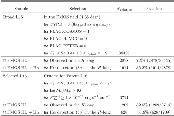
We refer to those satisfying all the above criteria as Pri-mary objects. From the COSMOS photometric catalog, 3876 objects are identified to meet the above criteria (the Primary-parent sample), and 1582 objects were ob-served in the H-long mode (the Primary-HL sample).
Figure 2 shows the SFR as a function of M∗ for the
parent sample (red contours), and the Primary-HL sample (blue circles). The observed objects trace the so-called main sequence (e.g., Noeske et al. 2007) of star-forming galaxies over two orders of magnitudes in stellar mass. However, the limit on the predicted Hα flux removed a substantial fraction (60 %) of poten-tial targets selected only with the KS and M∗ criteria
(shown by black dashed contours). In Figure2, we indi-cate median SFRs in bins of M∗ separately for the
Date (Local Time) Program ID Pointing Grating Total exp time (hr) 2012-03-12 UH-B3 HR4 H-long 5 2012-03-13 S12A-096 HR1 H-long 5 2012-03-14 S12A-096 HR2 H-long 4.5 2012-03-15 S12A-096 HR1 H-long 5 2012-03-16 S12A-096 HR3 H-long 4 2012-03-17 S12A-096 HR1 H-short 4 2012-03-18 UH-B5 HR1 J -long 4.5 2012-12-28 UH-18A HR2 J-long 3.5 2013-01-18 S12B-045I HR3 H-long 3 2013-01-19 S12B-045I HR4 H-long 3.5 2013-01-20 UH-18A HR3 J-long 4.5 2013-01-21 UH-18A HR4 J-long 3.5 2013-12-28 S12B-045I HR2 H-long 4.25 2014-01-21 UH-11A EXT1 H-long 2.25 2014-01-23 UH-11A EXT2 H-long 2 2014-01-24 S12B-045I HR3 H-long 1.5 2014-01-25 S12B-045I HR1 H-long 5.25 2014-01-26 S12B-045I HR4 H-long 5 2014-02-07 S12B-045I HR1 J-long 4.5 2014-02-08a S12B-045I HR4 J-long 5.5 2014-02-09a S12B-045I HR4 J-long 5 2014-02-10 UH-38A EXT3 H-long 5.5
aThese two J-long observations have been conducted with the same fiber allo-cation design (i.e., the same galaxies were observed in total 10.5 hours in the two nights.)
predicted Hα flux. It is shown that the limit on FHαpred results in the observed sample being biased ∼ 0.2 dex higher in the average SFR, at all stellar masses. We found that the Primary-HL sample includes 70 objects detected by Chandra X-ray observations (see Section
3.3) by checking counterparts. These X-ray-detected ob-jects are excluded for studies on the properties of a pure star-forming population.
In addition to the Primary sample, the FMOS-COSMOS catalog contains a substantial number of star-forming galaxies at z ∼ 1.6 not satisfying all the criteria described above. This is because the crite-ria were loosened down to M∗ ≥ 109.57 M and/or
FHαpred≥ 4 × 10⁻¹⁷ erg s−1 cm−2 for a part of runs, and
we also allocated substantial number of fibers through the program to those at z ∼ 1.6 identified in the pho-tometric catalog, but not satisfying all the criteria for the Primary objects. We refer to these objects ob-served with the H-long grating as the Secondary-HL sample, which contains 1242 objects. In Figure 3, we show the distributions of galaxy properties for both the Primary-HL and the Primary+Secondary-HL objects. The Secondary-HL sample includes objects with lower or higher zphot and/or lower M∗ outside the limits,
while the majority are those with FHαpred lower than the threshold.
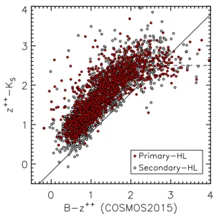
In Figure4, we show the Primary-HL and Secondary-HL objects in the (B − z) vs. (z − K) diagram.
Table 2. Summary of Subaru/FMOS HR observations (2014 March – 2016 April)
Date (Local Time) Program ID Pointing Grating Total exp time (hr) 2014-03-06 UH-38A EXT1 J-long 5.5 2014-12-02a UH-25A HR4E H-long 2.25 2015-02-08a S15A-134I HR7 H-long 4.5 2015-02-11a UH-22A HR7 H-long 5
2015-02-12a UH-22A HR6 H-long 3.5 2015-04-10a UH-22A HR5 H-long 4 2015-04-11a UH-22A HR5 H-long 1.5
2016-01-15 S15A-134I HR8E H-long 4.5 2016-01-16 S15A-134I HR4E H-long 4.5 2016-01-17 S15A-134I HR1E H-long 4.5 2016-01-18 UH-24A HRC0 H-long 5 2016-01-19 UH-24A HR6 H-long 5 2016-01-20 UH-24A HR7 J-long 5 2016-03-24 UH-11A HR1 J-long 3.5 2016-03-26 S16A-054I HR2 J-long 4.5 2016-03-27 S16A-054I HR4 J-long 4.5 2016-03-29 S16A-054I HR3 J-long 4 2016-03-30 S16A-054I HR7E H-long 4 2016-04-19 UH-11A HR1E J-long 3.25 2016-04-20 UH-11A HR6E J-long 3.5 2016-04-21 - 1st half S16A-054I HR1 J-long 3.5 (3.0 in IRS2) 2016-04-22 - 1st half S16A-054I HR3 J-long 3.5 2016-04-23 - 1st half S16A-054I HR2 J-long 3.25 2016-04-24 - 1st half S16A-054I HR8E J-long 3
aObservations from December 2014 to April 2015 have been conducted using only a single spectrograph IRS1.
These colors are based on the photometric measure-ments (Subaru B and z++, and UltraVISTA KS)
given in the COSMOS2015 catalog (Laigle et al. 2016). It is demonstrated that the majority (95%) of the Primary+Secondary-HL sample match the so-called sBzK selection (Daddi et al. 2004).
3.2. Far-IR sources from the Herschel PACS Evolutionary Probe (PEP) Survey
Herschel-PACS observations cover the COSMOS field at 100 µm and 160 µm, down to a 5σ detection limits of ∼ 8 mJy and ∼ 17 mJy, respectively (Lutz et al. 2011). These limits correspond to a SFR of roughly
100 M yr−1 at z ∼ 1.6. We allocated fibers to
these FIR-luminous objects for particular studies of star-burst and dust-rich galaxies (e.g.,Kartaltepe et al. 2015;
Puglisi et al. 2017) also in view of their follow-up with ALMA (Silverman et al. 2015a, 2018a,b). The objects were selected by cross-matching between the PACS Evo-lutionary Probe (PRP) survey catalog and the IRAC-selected catalog ofIlbert et al. (2010), and their stellar mass and SFR are derived from SED fits (further de-tailed in Rodighiero et al. 2011). For these objects, a higher priority with respect to fiber allocation had to be made since these objects are rare and would not be sufficiently targeted otherwise.
Figure 1. Upper panel: the FMOS pawprint overlaid on the HST/ACS mosaic of the COSMOS field (Koekemoer et al. 2007;Massey et al. 2010). Large circles show the FoV of each FMOS pointing. The central area of 0.81 deg2 covered by four FoVs (HR1–4) are highlighted by red. Lower panel: On-sky distribution of all galaxies in the FMOS-COSMOS catalog (gray circles). Red circles indicate those with any spectroscopic redshift estimate (1931 objects with zFlag ≥ 1; see Section5). The pawprints visited with the J -long grating are highlighted by thick blue circles.
Name R.A. Declination Nvisits Nvisits
(J2000) (J2000) H-long J -long HR1 09:59:56.0 +02:22:14 3 (+1)a 4 HR2 10:01:35.0 +02:24:52 2 3 HR3 10:01:19.7 +02:00:29 3 3 HR4 09:59:38.7 +01:58:08 3 3b HR1E 10:00:28.6 +02:37:49 1 1 HR2E 10:02: 1.4 +02:10:42 1 0 HR3E 09:58:48.2 +02:10:21 1 0 HR4E 10:02: 6.1 +02:37:12 2c 0 HR5E 10:01:51.1 +01:48:41 2c 0 HR6E 10:00:12.8 +01:47:39 2c 1 HR7E 09:58:28.6 +01:49:24 3c 1 HR8E 09:58:38.1 +02:35:45 1 1 HRC0 10:00:26.4 +02:12:36 1 0 Full aread 1.70 deg2
HR1–4e 0.81 deg2
a‘+1’ denotes an additional H-short observation.
b Two of the three J-long observations in HR4 have con-ducted with the same fiber allocation (i.e., observed the same galaxies in total 10.5 hours in two nights; see Table
1).
c Observations from 2014 Dec to 2015 Apr have been con-ducted with only a single spectrograph IRS1 (see Table
2).
dArea of the full FMOS-COSMOS survey field.
e Area covered by the central four FMOS pawprints (HR1– 4).
Our parent sample of the PACS sources contains 231 objects in the range 1.44 ≤ zphot≤ 1.72, and 116 objects
were selected for FMOS H-long spectroscopy. We refer to these objects as the PACS-HL sample. Figure2shows the distribution of the Herschel-PACS sample in the M∗
vs. SFR plot. It is shown that these objects are limited to be above an SFR of ∼ 100 M yr−1. Further analyses
of this subsample are presented in companion papers (Puglisi et al. 2017; Kartaltepe et al., in prep).
3.3. Chandra X-ray sources
We have dedicated a fraction of FMOS fibers to obtain spectra for optical/near-infrared counterparts to X-ray sources from the Chandra COSMOS Legacy
Figure 2. M∗ vs. SFR (from SED fits) for the target samples at z ∼ 1.6 in the FMOS-COSMOS survey. Red solid and
black dashed contours show the distribution (containing 68 and 90%) of the parent galaxies limited with (i.e., Primary-parent sample) and without the threshold FHαpred ≥ 1 × 10⁻¹⁶
erg s−1 cm−2. Correspondingly, yellow and white stars indicate the median SFRs in bins of M∗, respectively, for the parent galaxies with and without the limit on the predicted Hα flux. Objects
in the Primary-HL sample are indicated by blue circles, with X-ray detected objects marked by magenta diamonds. Orange empty and filled squares indicate the PACS-parent and PACS-HL samples (Section3.2).
Figure 3. From left to right, distributions of zphot, KS magnitude, M∗, and predicted FHα for the Primary-HL (red hatched
histograms) and the Secondary-HL (plus Primary-HL) sample (empty histograms). survey (Elvis et al. 2009; Civano et al. 2016). The
FMOS-COSMOS catalog includes 84 X-ray-selected ob-jects intentionally targeted as compulsory. However, there are many X-ray sources other than those, which have been targeted as star-forming galaxies (i.e., the Primary/Secondary-HL sample) or infrared galaxies. We thus performed position matching between the full FMOS-COSMOS catalog and the full Chandra
COS-MOS Legacy catalog1. In total, we found an X-ray
counterpart for 742 (including the intended 84 objects) among all FMOS extragalactic objects. Most of these X-ray-detected objects are probably AGN-hosting
galax-1 The Chandra catalogs are available here:
Figure 4. Primary-HL (red circles) and Secondary-HL (gray circles) samples in the BzK diagram. The solid and dashed lines indicate the boundaries for distinguishing z > 1.4 star-forming, z > 1.4 quiescent, and z < 1.4 galaxies, defined byDaddi et al.(2004).
ies. These objects are not included in the analyses pre-sented in the rest of this paper, but studies of these X-ray sources are presented in companion papers (Schulze et al. 2018, Kashino et al. in prep.).
3.4. Additional infrared galaxies
We also allocated a substantial number of fibers to observe lower redshift (0.7 . z . 1.1, where Hα falls in the J -long grating) infrared galaxies selected from S-COSMOS Spitzer-MIPS observations (Sanders et al. 2007) and Herschel PACS and SPIRE from the PEP (Lutz et al. 2011) and HerMES (Oliver et al. 2012) sur-veys, respectively. We used the photometric redshifts of Ilbert et al. (2015) and Salvato et al. (2011, for X-ray detected AGN) for the source selection. We derived the total IR luminosity, calculated from the best-fit IR template using the SED fitting code LePhare and in-tegrating from 8 to 1000 microns. These luminosities range between 1011
. LIR/L . 1012.5, spanning the
luminosity regime of LIRG/ULIRG (Luminous and Ul-traluminous Infrared Galaxies, see review bySanders & Mirabel 1996). Our parent sample includes 1818 objects between 0.66 ≤ zphot≤ 1.06. Of those, we observed 344
using the J -long grating. Further analysis of this par-ticular sub-sample will be presented in a future paper (Kartaltepe et al., in prep).
4. FLUX MEASUREMENT AND CALIBRATION
Our procedure for the emission-line fitting makes use of the IDL package mpfit (Markwardt 2009). Candi-date emission lines were modeled with a Gaussian pro-file, after subtracting the continuum. The Hα and [N ii] or Hβ and [O iii] lines were fit simultaneously while fix-ing the velocity widths to be the same and allowfix-ing no relative offset for the line centroids. The flux ratios of the doublet [N ii]λ6584/6548 and [O iii]λ5007/4959 were fixed to be 2.96 and 2.98, respectively (Storey & Zeippen 2000).
The spectral data processed with the standard reduc-tion pipeline, FIBRE-pac (Iwamuro et al. 2012), are given in units of µJy, which were converted into flux den-sity per unit wavelength, i.e., erg s−1 cm−2 ˚A−1, before fitting. The observed flux density Fλ,i, where i denotes
the pixel index, was fit with weights defined as the in-verse of the squared noise spectra output by the pipeline. The weights Wi were set to zero for pixels impacted by
the OH mask or sky residuals (see Figures 11 and 14 of
Silverman et al. 2015a).
We assessed the quality of the fitting results based on the signal-to-noise (S/N) ratio calculated from the formal errors on the model parameters returned by the mpfitfun code. We emphasize that these S/N ratios do not include the uncertainties on the absolute flux calibration described in later sections. In addition, we have also estimated the fraction of flux lost by bad pixels (i.e., pixels with Wi = 0). For all lines we define the ‘bad
pixel loss’ as the fraction of the contribution occupied by the bad pixels to the total integral of the Gaussian profile: fbadpix = P {i|Wi=0}Pi P iPi (1) where Piis the flux density of the best-fit Gaussian
pro-file at the ith pixel (not the observed spectrum). We disregard any tentative line detections if fbadpix> 0.7.
The goodness of the line fits is given by the reduced chi-squared statistic, χ2/dof where dof are the degrees of
freedom in the fits. Figure5shows the resultant χ2/dof
values as a function of line strength (upper panel) and of S/N (lower panel), separately for the Hα+[N ii] in H-long and Hβ+[O iii] in J-H-long. The distribution of the reduced χ2 statistics clearly peaks at χ2/dof ' 1, with no significant trends with either line strength or S/N.
In a relatively few cases, a prominent broad emission-line component was present and we included a sec-ondary, broad component for Hα or Hβ. Further-more, we also added a secondary narrow Hα+[N ii] (or Hβ+[O iii]) component with centroid and width differ-ent from the primary compondiffer-ent, when necessary (e.g., a case that there is a prominent blueshifted component
Figure 5. The reduced chi-squared statistic (χ2/dof) as a
function of observed line flux (upper panel) and S/N (lower panel). Left and middle panels show the results of fits to Hα+[N ii] in the H-long band, and Hβ+[O iii] in the J-long, respectively. Right panels show the corresponding normal-ized distributions of the χ2/dof values.
of the [O iii] line, possibly attributed to an outflow). Such exceptional handling was applied for only 5% of the whole sample (108 out of 1931 objects with a line detection). Most of these objects are X-ray detected and we postpone detailed analysis of these objects to a fu-ture paper, while focusing here on the basic properties of normal star-forming galaxies.
4.2. Upper Limits
For non-detections of emission lines of interest we es-timated upper limits on their in-fiber fluxes if we have a spectroscopic redshift estimate from any other detected lines in the FMOS spectra and the spectral coverage for undetected lines. The S/N of an emission line depends not only on the flux and the typical noise level of the spectra, but also on the amount of loss due to bad
pix-els. These effects have been considered on a case-by-case basis by performing dedicated Monte-Carlo simulations for each spectrum.
For each object with an estimate of spectroscopic red-shift, we created Nsim= 500 spectra containing an
arti-ficial emission line with a Gaussian profile at a specific observed-frame wavelength of undetected lines based on the zspec estimate. The line width was fixed to a
typi-cal FWHM of 300 km s−1 (Section 6.1), and Gaussian noise was added to these artificial spectra based on the processed noise spectrum. In doing so, we mimicked the impact of the OH lines and the masks. We then performed a fitting procedure for these artificial spectra with various amplitudes in the same manner as the data, and estimated the 2σ upper limit for each un-detected line by linearly fitting the sets of simulated fluxes and the associated S/Ns.
4.3. Integrated flux density
In addition to the line fluxes, we also measured the average flux density within the spectral window for in-dividual objects regardless the presence or absence of a line detection. The average flux density hfνi and the
as-sociated errors were derived by integrating the extracted 1D spectrum of each galaxy as follows.
hfνi = P ifν,iWiRi P iWiRidλ (2) ∆ hfνi = pP i(Nν,iWiRidλ)2 P iWiRidλ (3) where dλ = 1.25 ˚A is the wavelength pixel resolution, Ni
is the associated noise spectrum, and Ri is a response
curve.
Beside been used to estimate the equivalent widths of detected emission lines, these quantities can also allow for the absolute flux calibration by comparing them with the ground-based H or J -band photome-try. For this purpose, we use the fixed 300-aperture magnitudes H(J) MAG APER3 from the UltraVISTA-DR2 survey (McCracken et al. 2012) provided in the COS-MOS2015 catalog (Laigle et al. 2016) as reference, ap-plying the recommended offset from aperture to total magnitudes (see Appendix of Laigle et al. 2016). For comparison with the reference photometry, we define Ri
in the above equations based on the response curve of the VISTA/VIRCam H or J -band filters2, and flux den-sities were then converted to (AB) magnitudes. In the calculation of these equations, we did not exclude the de-tected emission lines because our primary purpose is to
2 The data for the filter response curves are available here:
Figure 6. Observed ‘raw’ HAB from the H-long
spec-tra vs. reference HABfrom the UltraVISTA. Red and blue
points correspond to the measurements with the two spec-trographs IRS1 and IRS2, respectively. Data points from a single observing run (2013-12-28) are highlighted with large symbols. A global offset of ∼ 1 mag from the one-to-one re-lation (dashed line) reflects the average aperture loss, while an offset of ∼ 0.5 mag between IRS1 (red) and IRS2 (blue) is due to the differential total throughput of these spectro-graphs.
compare these to the ground-based broad-band photom-etry, which in principle includes the emission line fluxes if exit3. We disregard the measurements with S/N < 5, and also exclude objects whose A- and/or B-position spectrum (obtained through the ABAB telescope nod-ding) falls on the detector next to those of flux standard stars since these spectra may be contaminated by leak-age from the neighbor bright star spectrum. Finally, we successfully measured the flux density for 2456 objects observed with the H-long grating, and for 1700 objects observed in J -long.
In Figure 6, we compared the observed magnitudes HAB from the FMOS H-long spectra with the
UltraV-ISTA H-band magnitudes, separately for the two spec-trographs (IRS1 and IRS2) of FMOS. Here the observed values were computed from spectra produced by the standard reduction pipeline, and we refer to these as the ‘raw’ magnitude. Data points from a single observ-ing run (2013-12-28) are highlighted for reference. It is clear that there is a global offset of ∼ 1 mag in the ob-served magnitudes relative to the reference UltraVISTA
3 For estimating the emission line equivalent widths, we
ex-cluded the emission line components.6.1.
Figure 7. Observed magnitude from the FMOS H-long (left panel) and J -long (right panel) spectra versus the esti-mated S/N. The data from IRS1 and IRS2 are shown sepa-rately with red and blue, respectively. The color solid lines are linear fits to the data, and horizontal lines indicate the threshold S/N = 5.
magnitudes. This reflects the loss flux falling outside the fiber aperture. In addition, we can also see that an ∼ 0.5 mag systematic offset exists between the two spectrographs. This offset is due to the difference in the total efficiency of the two spectrographs. Prior to the aperture correction, we first corrected for this offset between the IRS1 and IRS2, as follows:
HIRS1= HIRS1raw + (h∆H raw
IRS2i − h∆H raw
IRS1i)/2, (4)
HIRS2= HIRS2raw − (h∆H raw
IRS2i − h∆H raw
IRS1i)/2 (5)
where h∆Hraw
IRSii is the median offset of the observed
magnitude relative to the reference magnitude. This correction has been done for each observing run inde-pendently. We did the same for the J -band observations as well.
Figure7shows the observed magnitudes after correct-ing for the offset between IRS1 and IRS2. The mag-nitude from the H-long (left panel) and J -long (right panel) spectra are shown as a function of S/N ratios, separately for each spectrograph. The correlations are in good agreement between the two spectrographs, and between the spectral windows. The threshold S/N = 5 corresponds to ≈ 23.5 ABmag for both H and J .
We emphasize that, in the rest of the paper as well as in our emission-line catalog, the correction for the differ-ential throughput between the two IRSs is applied for all observed quantities, including emission-line fluxes, for-mal errors and upper limits on line fluxes. Therefore, catalog users do not need to care about this instrumen-tal issue. Meanwhile, the fluxes in the cainstrumen-talog denote the in-fiber values, hence the aperture correction should be
applied using the correction factors given in the catalog if necessary (see the next subsection for details).
4.4. Aperture correction
As already mentioned, the emission-line and broad-band fluxes measured from observed FMOS spectra arise from only the regions of each target falling within the 100.2-diameter aperture of the FMOS fibers. Therefore, it is necessary to correct for flux falling outside the fiber aperture to obtain the total emission line flux of each galaxy. The amount of aperture loss depends both on the intrinsic size of each galaxy and the conditions of the observation, which include variable seeing size and fluc-tuations of the fiber positions (typically ∼ 000.2;Kimura et al. 2010). We define three methods for aperture cor-rection.
First, the aperture correction can be determined by simply comparing the observed H (or J ) flux density obtained by integrating the FMOS spectra to the refer-ence broad-band magnitude for individual objects. This method can be utilized for moderately luminous objects for which we have a good estimate of the integrated flux from the FMOS spectra (observed HAB . 22.5). This
method cannot be applied for objects with poor contin-uum detection and suffering from the flux leakage from bright objects.
Second, we can use the average offset of the observed magnitude relative to the reference magnitude for each observing run. This method can be applied to fainter objects and those with insecure continuum measurement (e.g., impacted by leakage from a bright star) for cor-recting the emission line fluxes.
Lastly, we determine the aperture correction based on high-resolution imaging data. In the COSMOS field, we can utilize images taken by the HST/ACS (Koekemoer et al. 2007; Massey et al. 2010) that covers almost en-tirely the FMOS field and offers high spatial resolution. The advantage of this method is that we can determine the aperture correction object-by-object taking into ac-count their size property and a specific seeing size of the observing night. Hereafter we describe in detail this third method (see also Kashino et al. 2013; Silverman et al. 2015b).
For each galaxy, the aperture correction is determined from the HST/ACS IF814W-band images (Koekemoer
et al. 2007). In doing so, we implicitly assume that the difference between the on-sky spatial distributions of the rest-frame optical continuum (i.e., stellar radia-tion) and nebular emission is negligible under the typical seeing condition (& 0.5 arcsec in FWHM). This assump-tion is reasonable for the majority of the galaxies in our
sample, in particular, those at z > 1 whose typical size is < 1 arcsec.
We performed photometry on the ACS images of the FMOS galaxies using SExtractor version 2.19.5 (Bertin & Arnouts 1996). The flux measurement was per-formed at the position of the best-matched object in the COSMOS2015 catalog if it exists, otherwise at the position of the fiber pointing, with fixed aperture size. For the majority of the sample, we use the measure-ments in the 200-diameter aperture (FLUX APER2), but employed a 300 aperture (FLUX APER3) for a small frac-tion of the sample if the size of the object extends sig-nificantly beyond the 200aperture, and consequently, the ratio FLUX APER3/FLUX APER2 is & 1.34. We visually
in-spected the ACS images to check for the presence of sig-nificant contamination by nearby objects, flagging such cases in the catalog.
Next we smoothed the ACS images by convolving with a Gaussian point-spread function (PSF) for the effective seeing size. We then performed aperture photometry with SExtractor to measure the flux in the fixed FMOS fiber aperture FLUX APER FIB, and computed the correc-tion factor as caper = FLUX APER2(3)/FLUX APER FIB.
The size of the smoothing Gaussian kernel (i.e., the ef-fective seeing size) was retroactively determined for each observing run to minimize the average offset relative to the reference UltraVISTA broad-band magnitudes ( Mc-Cracken et al. 2012) fromLaigle et al.(2016) (see Section
4.3). We note that the effective seeing sizes determined are in broad agreement with the actual seeing conditions during the observing runs (∼ 000.5–100.4 in FWHM) that were measured from the observed point spread function of the guide stars.
Figure8shows the derived aperture correction factors as a function of the reference magnitude, separately for the H and J bands. We excluded insecure estimates of aperture correction, which includes cases where the blending or contamination from other objects are signif-icant. The aperture correction factors range from ∼ 1.2 to ∼ 4.5, and the median values are 2.1 and 2.5 for the H and J band, respectively. This small offset between the two bands is due to the fact that seeing is worse for shorter wavelengths under the same condition. Note that the formal error on the correction factor that comes from the aperture photometry on the ACS image (e.g.,
4In our previous studies (Kashino et al. 2013;Silverman et al.
2015b), the pseudo-total Kron flux FLUX AUTO was used as the total IF814W-band flux, rather than the fixed-aperture flux used
in this paper. Although the conclusions are not affected by the choice, the use of the fixed-aperture gives better reproducibility of photometry as the Kron flux measurement is more sensitive to the configuration to execute the SExtractor photometry.
Figure 8. Derived aperture correction factors caper as a
function of the reference H or J magnitudes (Laigle et al. 2016). The horizontal solid lines mark the median values. Histograms show the distribution of caper, separately for the
H- (red) and J -long (blue) bands.
FLUXERR APER2) is small (typically < 5%), and thus the scatter seen in Figure8is real, reflecting both variations in the intrinsic size of galaxies and the seeing condition of observing nights.
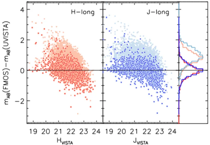
Figure9 shows offsets between the observed and the reference magnitudes before and after correcting for aperture losses, as a function of the reference magni-tudes. The average magnitude offset is mitigated by applying the aperture correction. After aperture correc-tion, we found that the standard deviation of the magni-tude offsets to be 0.42 (0.50) mag, after (before) taking into account the individual measurements errors in both hfνi of the observed FMOS spectra and the reference
magnitude. There is no significant difference between H and J . Note that this comparison also provides a sense of testing agreement between the first method of aperture correction estimation, described above, that re-lies on the direct comparison between the observed flux density on the FMOS spectra and the reference magni-tude.
In the catalog, we provide the best estimate of aper-ture correction for each of all galaxies regardless the presence or absence of spectroscopic redshift estimate. For 67% of the sample observed in the H-long spectral window and 80% in J -long, the best aperture correc-tion is based on the HST/ACS image described above. However, for the remaining objects, the estimates with this method are not robust due to blending, significant contamination from other sources, or any other trou-bles on pixels of the ACS images. Otherwise, there is no ACS coverage for some of those falling outside the area (see Figure 1). For such cases, we provide as the
Figure 9. The difference between the observed (FMOS) and reference (UltraVISTA;Laigle et al. 2016) magnitudes for the H- and J -bands. The pale and bright color points correspond respectively to before and after the aperture cor-rection being applied. The histograms show the distribution of the differential magnitudes separately for each band, as well as for before/after the correction.
best aperture correction an alternative estimate based on the second method that uses the average offset of all objects observed together in the same night. With these aperture correction, the agreement between the aperture-corrected observed flux density and the refer-ence magnitude is slightly worse, with an estimated in-trinsic scatter of ≈ 0.57 dex for both H- and J -long, than that based on the ACS image-based aperture cor-rection.
In the following, we use these best estimates of aper-ture correction without being aware of which method is used. Throughout the paper, when any aperture cor-rected values such as total luminosity and SFRs are shown, the error includes in quadrature a common fac-tor of 1.5 (or 0.17 dex) in addition to the formal error on the observed emission line flux to account for the intrinsic uncertainty of aperture correction. Lastly, we emphasize that the aperture correction is determined for all the individual objects using the independent ob-servations (i.e., HST/ACS and Ultra-VISTA photome-try) and just average information of the FMOS observa-tions (i.e., mean offset), but not relying on the individual FMOS measurements. This ensures that the uncertainty of aperture correction is independent of the individual FMOS measurements.
5. LINE DETECTION AND REDSHIFT ESTIMATION
The full FMOS-COSMOS catalog contains 5247 ex-tragalactic objects that were observed in any of three,
H-long, J -long, or H-short bands 5. The majority of
the survey was conducted with the H-long grating, col-lecting spectra of 4052 objects. The second effort was dedicated to observations in the J -long band, including the follow up of objects for which Hα was detected in H-long to detect other lines (i.e., Hβ and [O iii]) and observations for lower-redshift objects to detect Hα. A single night was used for observation with the H-short grating (see Table1). In this section, we report spectro-scopic redshift measurements and success rates.
5.1. Spectroscopic redshift measurements
Out of the full sample, we obtained spectroscopic red-shift estimates for 1931 objects. The determination of spectroscopic redshift is based on the detection of at least a single emission line expected to be either Hα, [N ii], Hβ, or [O iii]. For our initial target selection, galaxies were selected based on the photometric redshift zphot so that Hα+[N ii] and Hβ+[O iii] are detected in
either the H-long or J -long spectral window. For the majority of the sample, we identified the detected line as Hα or [O iii] according to their zphot. However, this is
not the case for a small number of objects for which we found a clear combination of Hα+[N ii], or [O iii] doublet (+Hβ) in a spectral window not expected from the zphot.
For objects observed both in H- and J -band, we checked whether their independent redshift estimates are consis-tent. If not, we re-examined the spectra to search for any features that can solve the discrepancy between the spectral windows. Otherwise, we disregarded line detec-tions of lower S/N. For objects observed twice or more times, we adopted a spectrum with the highest S/N ra-tio of the line flux. For objects with consistent line de-tections in the two spectral windows (i.e., Hα+[N ii] in H-long, and Hβ+[O iii] in J-long), we regarded a red-shift estimate based on higher S/N detection as the best estimate (zbest). There also objects that were observed
twice or more times in the same spectral window. In particular, the repeat J -long observations have been car-ried out to build up exposure time to detect faint Hβ at higher S/N. In the catalog presented in this paper, how-ever, we adopted a single observation with detections of the highest S/N ratio, instead of stacking spectra taken on different observing runs6.
5The full FMOS-COSMOS catalog is available here:
http://member.ipmu.jp/fmos-cosmos/fmos-cosmos_catalog_ 2019.fits
For more information, please refer to the README file:
http://member.ipmu.jp/fmos-cosmos/fmos-cosmos_catalog_ 2019.README
6The measurements based on co-added spectra are provided in
an ancillary catalog.
We assign a quality flag (zFlag) to each redshift es-timate based on the number of detected lines and the associated S/N as follows (see Section 4.1for details of the detection criteria).
zFlag 0 : No emission line detected.
zFlag 1 : Presence of a single emission line detected at 1.5 ≤ S/N < 3.
zFlag 2 : One emission line detected at 3 ≤ S/N < 5. zFlag 3 : One emission line detected at S/N ≥ 5.
zFlag 4 : One emission line having S/N ≥ 5 and a second line at S/N ≥ 3 that confirms the redshift. The criteria have been slightly modified from those used inSilverman et al. (2015b) (where Flag = 4 if a second line is detected at S/N ≥ 1.5). Note that objects with zFlag = 1 are not used for scientific analyses in the remaining of the paper.
In Table 4 we summarize the numbers of observed galaxies and the redshift estimates with the correspond-ing quality flags. In the upper three rows, the num-bers of galaxies observed with each grating are reported, while the numbers of galaxies observed in two or three bands are reported in the lower four rows. Table5 sum-marizes the number of galaxies with detections of each of four emission lines.
In the top panel of Figure10, we display the distribu-tion of all galaxies with a spectroscopic redshift estimate split by the quality flag. There are three redshift ranges, corresponding to possible combinations of the detected emission lines and the spectral ranges, as summarized in Table5. In the middle panel, we compare the distribu-tion of the FMOS-COSMOS galaxies to the redshift dis-tribution from the VUDS observations (Le F`evre et al. 2015). It is clear that our FMOS survey constructed a complementary spectroscopic sample that fills up the redshift gap seen in the recent deep optical spectroscopic survey. In the lower panel of Figure10, we show objects for which Hα is detected in the H-long spectra, with the positions of OH lines. Wavelengths of the OH lines are converted into redshifts based on the wavelength of the Hα emission line as zOH = λOH/6564.6˚A − 1. It is
clear that the number of successful detections of Hα is suppressed near OH contaminating lines. The OH sup-pression mask blocks about 30% of the H-band. This reduces the success rate of line detection.
Based on the full sample, we have a 37% (1931/5247) overall success rate for acquiring a spectroscopic redshift with a quality flag zFlag ≥ 1, including all galaxies ob-served in any of the FMOS spectral windows. We note
Spectra Wavelength range Nobs zFlag = 1 = 2 = 3 = 4 Total - 5247 140 389 507 895 H-long 1.60–1.80 µm 4052 117 314 384 694 H-short 1.40–1.60 µm 163 3 12 18 34 J -long 1.11–1.35 µm 2599 77 304 388 807 HL+HS - 108 3 9 13 28 HL+JL - 1441 54 229 266 607 HS+JL - 81 1 11 16 33 HL+HS+JL - 63 1 8 12 28
aThe numbers of observed galaxies in specified spectral window(s), i.e., zFlag ≥ 0.
Table 5. Summary of the emission-line detection
Line zmin–zmax 1.5 ≤ S/N < 3 3 ≤ S/N < 5 S/N ≥ 5
H-long Hα 1.43–1.74 111 305 909 [N ii] 1.43–1.73 298 274 247 Hβ 2.32–2.59 9 13 14 [O iii] 2.21–2.59 5 8 58 H-short Hα 1.26–1.46 2 1 21 [N ii] 1.31–1.46 2 5 6 Hβ 2.15–2.15 1 0 0 [O iii] 2.15–2.15 0 0 1 J -long Hα 0.70–1.05 13 50 267 [N ii] 0.70–1.04 44 74 134 Hβ 1.31–1.74 139 160 100 [O iii] 1.30–1.69 49 160 296
that given that only ∼ 70% of the H-band is available for line detection due to the OH masks, the effective success rate can be evaluated to be ∼ 37/0.7 = 53%. The full catalog, however, contains various galaxy pop-ulations selected by different criteria and many galax-ies may satisfy criteria for different selections, i.e., the subsamples overlap each other. In later subsections, we thus focus our attention separately to each of specific
subsamples of galaxies as described in Section3. In Ta-ble6, we summarize the successful redshift estimates for each subsample.
5.2. The primary sample of star-forming galaxies at z ∼ 1.6
The Primary-HL sample includes galaxies selected from the COSMOS photometric catalog, as described in Section 3.1. For these objects, our line identifica-tion assumed that the strongest line detected in the H-long band is the Hα emission line, although, for some cases, only the [N ii] line was measured and Hα was dis-regarded due to significant contamination on Hα. For other cases with no detections in the H-long window, the strongest line detection in the J -long spectra was assumed to be the [O iii]λ5007 line. We observed 1582 galaxies that satisfy the criteria given in Section3.1with the H-long grating, and successfully obtained redshift estimates with zFlag ≥ 1 for 749 (47%) of them. The measured redshifts range between 1.36 ≤ zspec ≤ 1.74.
Focusing on the detection of the Hα line in the H-long grating, we successfully detected it for 712 (643) at ≥ 1.5σ (≥ 3σ). We note that the remaining 37 objects includes [N ii] detections with the H-long grating, and Hβ and/or [O iii] detections with the J-long grating. In addition to the Primary objects, we also observed other 1242 star-forming galaxies at z ∼ 1.6 which do not match all the criteria for the Primary target (the Secondary-HL sample; see Section3.1). In Table 6, we summarize the number of redshift measurements for the Primary-HL and the Secondary-HL samples, as well as for the subset after removing X-ray detected objects.
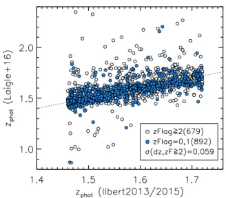
In Figure 11, we compare the the spectroscopic red-shifts with the photometric redred-shifts used for the
tar-Table 6. Summary of the Hα detection for the main subsamples
Hα detection Redshift quality flags Subsample Nobs 1.5 ≤ S/N < 3 3 ≤ S/N < 5 S/N ≥ 5 zF = 1 zF = 2 zF = 3 zF = 4
Primary-HL 1582 69 168 475 66 162 171 350
Primary-HL (X-ray removed) 1514 67 161 454 65 155 165 330
Secondary-HL 1242 34 91 255 32 96 109 182
Secondary-HL (X-ray removed) 1201 33 87 253 29 91 107 181
Herschel/PACS-HL 116 5 10 38 4 10 10 32
Low-z IR galaxies 344 3 20 149 5 24 35 124
Chandra X-ray objects 742 12 40 144 18 57 77 129
get selection from the photometric catalogs (Ilbert et al. 2013,2015) for the Primary-HL sample. For those with zFlag ≥ 2 (i.e., ≥ 3σ), the median and the standard deviation σstd of (zphot− zspec)/(1 + zspec) are −0.0099
(−0.0064) and 0.028 (0.024), respectively, after (before) taking into account the effects of limiting the range of photometric redshifts (1.46 ≤ zphot ≤ 1.72). To
ac-count for the edge effects, we adopted a number of sets of the the median offset and σstd to simulate
photomet-ric redshift for each zspecmeasurement, and then
deter-mined the plausible values of the intrinsic median and σstdthat can reproduce the observed median offset and
σstdof (zphot− zspec)/(1 + zspec) after applying the limit
of 1.46 ≤ zphot≤ 1.72.
5.3. The Herschel/PACS subsample at z ∼ 1.6 The PACS-HL sample include 116 objects between 1.44 ≤ zphot≤ 1.72 detected in the Herschel-PACS
ob-servations (Section3.2). We successfully measured spec-troscopic redshifts for 56 (43%) objects with zFlag ≥ 1, including 32 (28%) secure measurements (zFlag = 4). These measurements include 43 (3, 2) detection of Hα (≥ 3σ) in the H-long (H-short, J -long) band, as well as a single higher-z object with a possible detection of the [O iii] doublet in the H-long band (zspec= 2.26).
5.4. Lower redshift sample of IR luminous galaxies We observed in the J -long band 344 lower redshift galaxies selected from the infrared data (see Section3.4), and succeeded to measure spectroscopic redshift with zFlag ≥ 1 for 188 objects (55%). We detected the Hα emission line at S/N ≥ 1.5 (≥ 3.0) for 172 (169) objects. We note that 6 objects have detection of Hβ+[O iii] in the J-long, thus not being within the lower redshift win-dow.
5.5. Chandra X-ray sample
We observed in total 742 objects detected in the X-ray from the Chandra COSMOS Legacy survey (Elvis et al. 2009; Civano et al. 2016). Of them, 385 and 533 objects were observed with the H-long and J -long grat-ings, while 177 were observed with both of these. We obtained a redshift estimate for 281 (263) objects with zFlag ≥ 1 (≥ 2). The entire sample of the X-ray objects include 75 lower redshift (0.72 ≤ zspec ≤ 1.1) objects
with a detection of Hα+[N ii] in the J-long band, and 29 (1) higher redshift (2.1 ≤ zspec ≤ 2.6) objects with
a detection of Hβ+[O iii] in the H-long (H-short). The remaining majority of the sample are those at interme-diate redshift range with detections of Hα+[N ii] in the H-long band, and/or Hβ+[O iii] in the J-long band.
6. BASIC PROPERTIES OF THE EMISSION LINES 6.1. Observed properties of Hα
In Figure12we plot the observed in-fiber Hα flux FHα
(neither corrected for dust extinction nor aperture loss) as a function of associated S/N for each galaxy in our sample, split by the spectral window. As naturally ex-pected, there is a correlation between FHαand S/N, but
with large scatter in FHα at fixed S/N. This is mainly
due to the presence of ‘bad pixels’ impacted by OH masks and residual sky emission (see Section4.1). The figure indicates that, in the H-long band, the best sensi-tivity achieves FHα∼ 10−17 erg s−1 cm−2 at S/N = 3,
while the average is ∼ 3 × 10⁻¹⁷ erg s−1 cm−2.
In Figure 13, we show the correlation between FHα
(corrected for aperture, but not for dust) and the full width at half maximum (FWHM) of the Hα line in ve-locity units for galaxies with an Hα detection (≥ 3.0σ) in the H-long band (1.43 ≤ zspec ≤ 1.74). The
instrumen-Figure 10. Distribution of spectroscopic redshift measure-ments for all objects in the full FMOS-COSMOS catalog, split by their quality flags. The FMOS zspecdistribution is
compared with VUDS (Le F`evre et al. 2015, gray histograms) in the middle panel. The bottom panel shows zoom-in of the range 1.42 ≤ z ≤ 1.76 with a finer binsize (∆z = 0.002) for objects with an Hα detection in the H-long band. His-tograms are color-coded by S/N(Hα) as labeled. The gray stripes indicate positions of the OH airglow lines, which are converted to redshift with the wavelength of Hα.
Figure 11. Upper panel: comparison between zspec and
zphot for the Primary-HL sample. Each point is color-coded
by the quality flag of the redshift estimate, as labeled in the lower panel. Circles indicate the FMOS objects selected based on the photometric redshift fromIlbert et al.(2013), while squares indicate the objects based on Ilbert et al.
(2015). Lower panel: distribution of the differences between the spectroscopic redshifts from FMOS and the photometric redshifts.
tal velocity resolution (≈ 45 km s−1 at z ∼ 1.6). Al-though there is a weak correlation between these quan-tities, the line width becomes nearly constant at FHα&
1 × 10⁻¹⁶ erg s−1 cm−2. The central 90 percentiles of the observed FWHM is 108–537 km s−1 with the
me-Figure 12. Observed Hα flux (neither corrected for the aperture loss nor extinction) as a function of observed for-mal S/N for individual galaxies, shown separately for each spectral window as labeled. Vertical dashed lines indicates S/N = 1.5 (limit for detection), 3 (limit for zFlag = 2), and 5 (limit for zFlag = 3).
Figure 13. Correlation between aperture-corrected Hα flux (not corrected for dust) and line width (FWHM) in ve-locity units. The sample shown here is restricted to those with an Hα detection at 3 ≤ S/N < 5 (magenta) and S/N ≥ 5 (blue) in H-long (1.43 ≤ z ≤ 1.74). The horizontal line indicates the velocity resolution limit (45 km s−1).
dian at 247 km s−1. Limiting to those with FHα ≥
1 × 10⁻¹⁶ erg s−1 cm−2, the median is 292 km s−1. In Figure 14, we show the rest-frame equivalent width (EW0) of the Hα emission line as a function of
aperture-corrected continuum flux density hfλ,coni
aver-aged across the H-long spectral window. The continuum flux density was computed with Equation 2, excluding the emission line components. The equivalent widths were not corrected for differential extinction between
Figure 14. Rest-frame Equivalent width EW0(Hα) as a
function of aperture-corrected, average continuum flux den-sity hfλ,coni. Objects shown are limited to have both Hα
detection (≥ 3σ) and reliable continuum detection (≥ 5σ). Symbols are the same as in Figure13.
stellar continuum and nebular emission. The 759 ob-jects shown here are limited to have a detection of Hα at ≥ 3σ in H-long and a secure measurement of the contin-uum level (≥ 5σ). The observed EW0(Hα) ranges from
≈ 10 to 300 ˚A with the median hEW0(Hα)i = 71.7 ˚A.
The sample shows a clear negative correlation between hfλ,coni and EW0(Hα). The continuum and Hα flux
reflect, respectively, M∗ and SFR. Thus, this
corre-lation may be shaped by the facts that specific SFR (sSFR = SFR/M∗) decreases on average with M∗.
In Figure 15, we plot the observed Hα luminosity, LHα (corrected for aperture loss, but not for dust
ex-tinction), as a function of redshift, separately in the two redshift ranges that correspond to where Hα is de-tected (J -long or H-long/short). The observed LHα is
a weak function of redshift, increasing towards higher redshift, as shown by the linear regression that is de-rived in each range. This trend is almost negligible com-pared to the range spanned by the sample (∆z ≈ 0.4 each). For objects with an Hα detection (≥ 3σ) in the H-long spectral window, the central 90th percentiles of LHα is 1041.7–1042.7 erg s−1 with median hLHαi =
1042.25 erg s−1.
6.2. Sulfur emission lines
The Sulfur emission lines [S ii]λ6717,6731 fall in the H-long (J -long) spectral window together with Hα at 1.43 < z < 1.68 (0.70 < z < 1.00). For those with a detection of Hα and/or [N ii], we fit the [S ii] lines at the fixed spectroscopic redshift determined from Hα+[N ii], as described inKashino et al.(2017a).
Figure 15. Observed Hα luminosity (corrected for aper-ture loss, but not for dust extinction) as a function of redshift in the two redshift ranges, corresponding to the Hα detec-tion in J -long (left panel) and H-long/short (middle panel). The solid lines indicate the linear regression, being fitted in-dependently in each redshift range. Histograms show the normalized distribution of LHα for each redshift range as
color-coded (right panel).
Table 7. Summary of the detections (≥ 3σ) of the [S ii]λλ6717,6731 lines
Subsample criteria [S ii]λ6717 [S ii]λ6731 Both
Any 146 111 55
in H-long 98 72 30
in J -long 47 39 25 w/ Hα (≥ 3σ) in HL 84 54 22
We successfully detected the [S ii] lines for a substan-tial fraction of the sample. Table 7 summarizes detec-tions of the [S ii] lines. In total, we detected [S ii]λ6717 and [S ii]λ6731 at ≥ 3σ for 146 and 111 objects, respec-tively, with 55 with both detections at ≥ 3σ (see the top row in Table 7). Limiting those to have an Hα detec-tion (> 3σ) in H-long, we detected [S ii]λ6717 for 84, [S ii]λ6731 for 54, and both of these for 22 objects (all at ≥ 3σ). In Figure 16, we show the observed fluxes of [S ii]λ6717 and [S ii]λ6731 as a function of observed Hα flux, neither corrected for dust nor aperture loss. The observed flux of the single [S ii] line is on aver-age ≈ 1/5 times the observed Hα flux, ranging from F[SII]≈ 4 × 10⁻¹⁸ to 8 × 10⁻¹⁷ erg s−1 cm−2.
Figure 16. Correlation between observed Hα and [S ii] fluxes detected in the H-long band, neither corrected for aperture effects nor extinction. Red and blue filled (open) circles indicate the [S ii]λ6717 and [S ii]λ6731 fluxes with S/N ≥ 3 (1.5 ≤ S/N < 3), respectively. The diagonal solid line indicates the relation of F[SII]= FHα/5.
7. ASSESSMENT OF THE REDSHIFT AND FLUX MEASUREMENTS
7.1. Redshift accuracy
To evaluate the accuracy of our redshift estimates, we compared spectroscopic redshifts measured from Hα+[N ii] detected in the H-long spectra and those measured from Hβ+[O iii] in the J-long spectra. In the top panel of Figure 17, we show the distribution of (zH− zJ)/(1 + zbest) for 350 galaxies with
indepen-dent line detections in the two spectral windows both at ≥ 3σ. Of these, 172 objects have detections both at ≥ 5σ. Here, the best estimate of redshift zbest is
based on a detection with a higher S/N between the two spectral windows. The standard deviation σstd of
dz/(1 + z) is 3.3 × 10⁻⁴ for objects with ≥ 3σ detection (σstd= 2.2 × 10⁻⁴for ≥ 5σ), with a negligibly small
me-dian offset (2.6×10⁻⁵). The estimated redshift accuracy σstd/
√
2 is thus to be ≈ 70 km s−1.
An alternative check of redshift accuracy can be done using objects that have been observed twice or more times with the same grating on different nights. For these objects, we have selected the best spectrum to construct the line measurement catalog. However, the “secondary” measurements can be used to evaluate the
Figure 17. Upper panel: distribution of (zH − zJ)/(1 +
zbest), the difference between spectroscopic redshifts
mea-sured from Hα+[N ii] detected in the H-long and those from Hβ+[O iii] in the J-long spectra. The red histogram rep-resents the subsample with a ≥ 5σ detection in both H-and J -long spectra. Lower panel: distribution of (z2nd−
zprim)/(1 + zbest) (see text). Red and blue histograms
corre-spond independently to the measurements in the H-long and J -long, respectively. Here, the line detections are limited to be ≥ 3σ. In each panel, the values of standard deviation are denoted.
“primary” ones. In the lower panel of Figure 17, we show the distribution of the difference between the pri-mary (zprim) and the second-best (z2nd) redshift
mea-surements, separately for measurements obtained in H-long (29 objects) and in J -H-long band (113). Objects
are limited to those with ≥ 3σ detection in the pri-mary and secondary spectra. The standard deviation σstd of (z2nd − zprim)/(1 + zbest), reported in the
fig-ure for both H-long (σstd = 3.5 × 10⁻⁴) and J -long
(σstd = 3.3 × 10⁻⁴) observations, is similar to that
es-timated by comparing the H-long and J -long measure-ments.
7.2. Flux accuracy, using repeat observations The secondary measurements can be also used to eval-uate the accuracy of emission-line flux measurements. In Figure18, we compare the secondary and primary mea-surements of the Hα flux in the H-long window (upper panel; 24 objects), and the Hβ (middle panel; 58 ob-jects) and [O iii]λ5007 fluxes (lower panel; 109 obob-jects) in the J -long window. Because the two measurements are based on spectra taken under different seeing con-ditions, the aperture correction needs to be applied for comparison. We remind that the aperture correction is evaluated once for each object and observing night. It is shown that the primary and secondary measurements are in good agreement, as well as that aperture correc-tion improves their agreement as shown by histograms in the inset panels. We found the intrinsic scatter of these correlations to be 0.19, 0.21, and 0.19 dex for Hα, Hβ, and [O iii], respectively, after taking into account the effects of the individual formal errors of the observed fluxes. These intrinsic scatters should be attributed to the uncertainties of the aperture corrections, and indeed similar to the estimates made in Section4.4(see Figure
9).
7.3. Comparison with MOSDEF
Part of our FMOS-COSMOS targets were observed in the MOSFIRE Deep Evolution Field (MOSDEF) survey (Kriek et al. 2015). The latest public MOSDEF cata-log, released on 11 March 2018, contains 616 objects in the COSMOS field. Cross-matching with the FMOS catalog, we found 45 sources included in both catalogs, and of these, 15 objects have redshift estimates in both surveys.
Among the matching objects, all 11 FMOS measure-ments with zFlag = 4 and a single zFlag = 3 agree with the MOSDEF measurements, which all have a quality flag (Z MOSFIRE ZQUAL) of 7 (based on multiple emis-sion lines at S/N ≥ 2). The three inconsistent mea-surements are as follows. An object (zFMOS = 1.515
with zFlag = 3) has a [O iii] detection at > 5σ, with a possible consistent detection of Hα, in the FMOS spectra, while the MOSDEF measurement is z = 2.1 with a flag of 7. The photometric redshift zphot =
measure-Figure 18. Comparison of the best (primary) and the second best (secondary) measurements of the Hα flux in the H-long (top panel), and Hβ and [O iii]λ5007 fluxes in the J -long window (middle and bottom panels) for the repeated objects. Red and gray circles indicate the observed fluxes with and without aperture correction. Inset panels show the distribution of the flux ratios log(Fsecond/Fprimary) before
(gray) and after (red hatched histogram) aperture correction.
mates (flags) are zFMOS/MOSDEF = 1.581/2.555 (2/6)
and zFMOS/MOSDEF = 1.584/2.100 (1/7), respectively),
the detections of Hα on the FMOS spectra are not robust, both being significantly affected by the OH mask. The photometric redshift prefers zMOSDEF for
the former (zphot = 2.612), while zFMOS for the
lat-ter (zphot = 1.458). We note that the redshift range
of the MOSDEF survey is 1 . z . 3.5, but having a higher sampling rate at 2 < z < 2.6. Therefore, it is not straightforward to estimate the failure rate in our survey, which could be overestimated. The small sample size of the matching objects also makes it difficult. However, we could conclude that, for objects with zFlag=3 and 4, the failure rate should be below 10% (1/13 = 7.7%).
For these 12 consistent measurements, we found the median offset and standard deviation of (zFMOS −
zMOSDEF)/(1+zMOSDEF) to be −1.63×10⁻⁵(4.9 km s−1)
and 2.57 × 10⁻⁴ (77 km s−1). This indicates that there is no significant systematic offset in the wavelength cal-ibration of the FMOS survey relative to the MOSDEF survey.
7.4. Comparison with 3D-HST
A part of the CANDELS-COSMOS field (Grogin et al. 2011) is covered by the 3D-HST survey (Brammer et al. 2012), which is a slitless spectroscopic survey using the HST/WFC3 G141 grism to obtain near-infrared spec-tra from 1.10 to 1.65 µm. This configuration yields detections of Hα and [O iii] lines for those matched to the FMOS catalog. For redshift and flux comparisons with our measurements, we employed the public ‘line-matched’ catalogs (ver. 4.1.5) for the COSMOS field (Momcheva et al. 2016), in which the spectra extracted from the grism images were matched to photometric tar-gets (Skelton et al. 2014)7. Cross-matching the 3D-HST
and the FMOS catalogs, we found 78 objects that have redshift measurements from both surveys. We divided these objects into two classes according to the quality flags in the 3D-HST catalog (flag1 and flag2). The ‘good’ class contains 67 objects with both flag1 = 0 and flag2 = 0, while the remaining 11 objects are clas-sified to the ‘warning’ class.
In Figure 19, we compare our FMOS redshift es-timates to those from 3D-HST for the 78 matching sources. The colors indicate the quality flags of the FMOS measurements (see Section5.1) and the symbols correspond to the quality classes of the 3D-HST mea-surements as defined above. In the inset panel, we show the distribution of (zFMOS− z3DHST)/(1 + z3DHST) for


![Figure 20. Comparison of the fluxes of Hα (+[N ii ]) (up- (up-per panel), and Hβ and [O iii ] (lower panel) measured by FMOS and 3D-HST](https://thumb-eu.123doks.com/thumbv2/123doknet/14793499.602535/22.918.110.425.112.415/figure-comparison-fluxes-panel-lower-panel-measured-fmos.webp)

![[The framing on human stem cells research under the screen of French Parliament]](data:image/gif;base64,R0lGODlhAQABAIAAAP///wAAACH5BAEAAAAALAAAAAABAAEAAAICRAEAOw==)