Quality assessment of water cycle parameters in REMO by Radar-Lidar synergy

HAL Id: hal-00302881

https://hal.archives-ouvertes.fr/hal-00302881

HAL is a multi-disciplinary open access

archive for the deposit and dissemination of sci-entific research documents, whether they are pub-lished or not. The documents may come from teaching and research institutions in France or abroad, or from public or private research centers.

L’archive ouverte pluridisciplinaire HAL, est destinée au dépôt et à la diffusion de documents scientifiques de niveau recherche, publiés ou non, émanant des établissements d’enseignement et de recherche français ou étrangers, des laboratoires publics ou privés.

Quality assessment of water cycle parameters in REMO

by Radar-Lidar synergy

B. Hennemuth, A. Weiss, J. Bösenberg, D. Jacob, H. Linné, G. Peters, S.

Pfeifer

To cite this version:

B. Hennemuth, A. Weiss, J. Bösenberg, D. Jacob, H. Linné, et al.. Quality assessment of water cycle parameters in REMO by Radar-Lidar synergy. Atmospheric Chemistry and Physics Discussions, European Geosciences Union, 2007, 7 (3), pp.8455-8524. �hal-00302881�

ACPD

Full Screen / Esc

Printer-friendly Version

Interactive Discussion Atmos. Chem. Phys. Discuss., 7, 8455–8524, 2007

www.atmos-chem-phys-discuss.net/7/8455/2007/ © Author(s) 2007. This work is licensed

under a Creative Commons License.

Atmospheric Chemistry and Physics Discussions

Quality assessment of water cycle

parameters in REMO by Radar-Lidar

synergy

B. Hennemuth1,*, A. Weiss2, J. B ¨osenberg1, D. Jacob1, H. Linn ´e1, G. Peters3, and S. Pfeifer1

1

Max-Planck-Institute for Meteorology, Hamburg, Germany

2

British Antarctic Survey, High Cross, Madingley Road, Cambridge CB3 0ET, UK

3

Meteorological Institute, University of Hamburg, Hamburg, Germany

*

now: Consulting Meteorologist, Hamburg, Germany

Received: 30 May 2007 – Accepted: 1 June 2007 – Published: 20 June 2007 Correspondence to: B. Hennemuth (hennemuth@dkrz.de)

ACPD

Full Screen / Esc

Printer-friendly Version

Interactive Discussion

Abstract

A comparison study of water cycle parameters derived from ground-based remote-sensing instruments and from the regional model REMO is presented. Observational data sets were collected during three measuring campaigns in summer/autumn 2003 and 2004 at Richard Aßmann Observatory, Lindenberg, Germany. The remote sensing

5

instruments which were used are differential absorption lidar, Doppler lidar, ceilometer, cloud radar, and micro rain radar for the derivation of humidity profiles, ABL height, water vapour flux profiles, cloud parameters, and rain rate. Additionally, surface latent and sensible heat flux and soil moisture were measured. Error ranges and represen-tativity of the data are discussed. For comparisons the regional model REMO was run

10

for all measuring periods with a horizontal resolution of 18 km and 33 vertical levels. Parameter output was every hour. The measured data were transformed to the vertical model grid and averaged in time in order to better fit with gridbox model values. The comparisons show that the atmospheric boundary layer is not adequately simulated, on most days it is too shallow and too moist. This is found to be caused by a wrong

15

partitioning of energy at the surface, particularly a too large latent heat flux. The reason is obviously an overestimation of soil moisture during drying periods by the one-layer scheme in the model. The profiles of water vapour transport within the ABL appear to be realistically simulated. The comparison of cloud cover reveals an underestimation of low-level and mid-level clouds by the model, whereas the comparison of high-level

20

clouds is hampered by the inability of the cloud radar to see cirrus clouds above 10 km. Simulated ABL clouds apparently have a too low cloud base, and the vertical extent is underestimated. The ice water content of clouds agree in model and observation whereas the liquid water content is unsufficiently derived from cloud radar reflectivity in the present study. Rain rates are similar, but the representativeness of both

observa-25

ACPD

Full Screen / Esc

Printer-friendly Version

Interactive Discussion

1 Introduction

Regional climate models are widely used to assess regional climatic features for present climate and increasingly also for future climate, e.g. to downscale global change scenarios for the analysis of regional climate change and its impacts. For these studies, validation of the model, e.g. comparisons of model simulations with

observa-5

tions are an essential prerequisite to ensure that the main processes are simulated properly. One of the key processes is the water cycle, controlling cloud formation and precipitation. Of special interest are cloud parameters because of their strong impact on radiation, and thus on energetic issues. Moreover, the formation of precipitation is a crucial point for the assessment of climate. Special interest should also be directed to

10

boundary layer parameters because of the great turnover of water and energy in this layer adjacent to the earth’s surface.

Ground-based remote sensing systems are adequate instrumentation for model comparison of water cycle parameters since a lot of quantities can be derived, and they cover a wide range of heights and operate continuously. There has been

enor-15

mous progress in the development and refinement of ground-based remote sensing instruments for the determination of humidity, wind, cloud parameters and rain rate in recent years (e.g.,B ¨osenberg and Linn ´e,2002;Bormotov et al.,2000;Haeffelin et al.,

2005; Peters et al., 2002; Intrieri et al., 2002), and also the retrieval algorithms for

characterising clouds have been much improved in recent years, not least because

20

of international projects like BALTEX BRIDGE with its subprogrammes CLIWA-NET and 4D CLOUDS (e.g., Crewell et al., 2004;L ¨ohnert et al., 2004), and CLOUDNET (http://www.cloud-net.org/). In particular the CLOUDNET project has promoted the re-trievals of cloud liquid water and cloud ice water content (e.g.,Tinel et al., 2005;Liu

and Illingworth,2000;Hogan et al.,2006).

25

Many model validation studies concentrate on single parameters such as evapora-tion, precipitaevapora-tion, boundary layer height, or cloud parameters (e.g., Chiriaco et al.,

observa-ACPD

Full Screen / Esc

Printer-friendly Version

Interactive Discussion tions are available with a good resolution due to a dense rain gauge network over land

and radar networks e.g. over the Baltic Sea region (Jacob,2001). Within CLOUDNET and CLIWA-NET extensive comparisons of the observed cloud structure with several operational forecast models like ECMWF model, RACMO, RCA and LM with horizontal resolution between 50 km and 7 km were performed (Will ´en et al.,2005).

5

In this study water cycle parameters measured at the Meteorological Observatory Lindenberg (MOL), Germany, during experiments in summer and autumn 2003 and 2004 are compared with simulated parameters of the regional model REMO. The com-parisons include vertical distribution of humidity in the lower troposphere, surface evap-oration, soil moisture, profiles of vertical water vapour flux in the boundary layer, cloud

10

cover, vertical distribution of cloud boundaries, cloud water and ice, and precipitation. Special attention is paid to the atmospheric boundary layer (ABL), particularly to the convective boundary layer (CBL) because of its important role in controlling the water transport between the earth’s surface and the free atmosphere. The data set is used for statistical analysis as well as for process studies. Special emphasis is given on the

15

assessment of the differences between observed and modelled values with regard to measurement accuracy.

2 Instrumentation, measured parameters and accuracy

2.1 Lidar systems Water vapour lidar

20

The MPI-DIAL (Differential Absorption Lidar) is a vertically pointing water vapour lidar. It combines signals at two slightly different wavelengths. One wavelength is located in the centre of a water vapour absorption line (“online”), the other is located just beside but in a region of negligible water vapour absorption (“offline”). The backscatter coef-ficient can be assumed to be the same for both wavelengths, so the ratio of the two

ACPD

Full Screen / Esc

Printer-friendly Version

Interactive Discussion signals depends only on water vapour absorption. For details of the methodology the

reader is referred toB ¨osenberg (1998, 2005). Typical performance values are sum-marised in Table1, but lower resolution and/or decreased accuracy may occur in the upper altitude range. The measurement error caused by noise is nearly constant with height within the boundary layer and strongly increases in the free atmosphere. Table1

5

gives the error range within the boundary layer.

The backscatter measurement has a vertical resolution of 15 m.

During the first campaign a different laser type was used (Wulfmeyer and B ¨osenberg,

1998) than in the later campaigns (Ertel,2004). Due to the different configuration and adjustment the height interval was 700 m to 4000 m in 2003 and 300 m to 3000 m in

10

2004. The operating time was daytime only. Doppler lidar

For vertical wind speed measurements a Doppler lidar (MPI Hamburg) with heterodyne detection, operating at 1120 nm wavelength was used. The instrument is decribed by

Linn ´e et al. (2006). The performance depends on the presence of aerosol particles

15

of sufficient size to produce backscatter at the operating wavelength of 1120 nm, so wind data are collected in the boundary layer mainly. Typical performance values are summarised in Table1. The noise induced error estimated from the power spectrum is less than 0.1 m s−1within the boundary layer. Both lidar systems, DIAL and Doppler lidar were only operated during daytime because unattended operation was not feasible

20

at that time. Ceilometer

The Laser-Ceilometer Tropopauser LD40 (Impulsphysik GmbH) measures cloud base heights. Only standard products of the online signal processing software were used which include the detection of up to three cloud levels, depending on cloud optical

25

ACPD

Full Screen / Esc

Printer-friendly Version

Interactive Discussion 2.2 Radar systems

Cloud radar

The cloud radar MIRA-36 (METEK GmbH) is a vertically pointing Doppler radar, mea-suring at a frequency of 36.5 GHz corresponding to 8 mm wavelength (Bormotov et al.,

2000). It provides the radar reflectivity factorZ which is equal to the 6th moment of

5

the drop size distributionN(D) for drops with diameter D≪λ (Rayleigh approximation). In addition to Z, the Doppler velocity V and the linear depolarization ratio LDR are recorded since these variables are useful for target classification. Main operating pa-rameters of the radar are given in Table2. The cloud radar was operating continuously. The interpretation of radar reflectivities in terms of cloud properties requires some

10

caution since signals at the radar receiver input are not necessarily due to cloud echoes. Figure1 shows frequency distributions of 10· log(Z) (= : dBZ for shortness) with units ofZ=mm6/m3 for four height intervals between 2 and 10 km for the whole analysis period described in Sect. 4.1. At all heights the distributions exhibit two or even three modes.

15

The modes at the low end of theZ-distributions are not related to clouds but to the noise floorP_nof the radar receiver. In the signal analysis implemented during the cam-paignsPnwas set equal to the receiver input power observed at 12 km range, where no echo is expected. The corresponding noise spectra are assumed to be frequency in-dependent, and are subtracted from the spectra measured at lower heights in order to

20

obtain noise corrected signal powers. The estimated spectral noise floor is distributed randomly around the noise expectation value with the standard deviationσn=hPni/F0.5 where hPni is the expectation value of Pn and F =SfSt is the number of degrees of freedom withS_f andS_t number of spectral lines and number of spectral averages, re-spectively. As the noise at 12 km is not correlated with noise at other sounding heights,

25

the random fluctuations of the noise corrected receiver power represent (in the ab-sence of echoes) a zero-mean distribution with the standard deviation σ_nc=20.5· σn. Only the positive wing of this distribution is displayed on the logarithmic axis. It gives

ACPD

Full Screen / Esc

Printer-friendly Version

Interactive Discussion rise to the sharp peaks at the low end of theZ-distributions. These peak positions are

shifted to higherZ with increasing height z according to the geometric signal atten-uation proportional toz2. The correspondingZ-values were discarded by setting the detection threshold such that the false alarm rate is less than 5%.

The peaks at the high end of theZ-distributions, which appear in the lower two height

5

intervals, are due to drizzle, while the broad maximum around –40 dBZ occurring in the lowest height interval is influenced by atmospheric particles (see Sect.2.8) that gives rise to weak but rather persistent echoes in the atmospheric boundary layer. Only the peaks at –20 dBZ (6–8 km) and at –35 dBZ (8–10 km) are believed to stem actually from cloud droplets. These potential ambiguities underline the need of further information in

10

order to derive sensible cloud statistics. As discussed in Sect.2.8, simultaneous lidar echoes were used in this study to remove efficiently the boundary-layer particle signal. In the same way drizzle induced ambiguities were mitigated – however at this stage only with regard to cloud base detection, but not to liquid water estimation.

Micro Rain Radar

15

The micro rain radar MRR (METEK GmbH) measures the size distribution of rain droplets at 32 heights from which rain parameters, including the rainrate, can be de-rived (Peters et al., 2002,2005). The measuring frequency is 24.1 GHz. The height interval was 50 m in 2003 and 100 m in 2004. The lowest useful height is the third range gate (150 m/300 m) which was used in this study. The retrieval of size distribution is

20

based on the size-dependent terminal fall velocity of rain drops. Vertical air motion is the dominating source of error. In terms of rain rate the error is 25% per 0.1 m s−1 ver-tical wind. For 1 min averages the estimated standard deviation of the statisver-tical rain rate error is±20% under conditions typical for these data sets.

ACPD

Full Screen / Esc

Printer-friendly Version

Interactive Discussion 2.3 Other instrumentation

In the area around MOL a network of global radiation instruments and of 14 PLUVIO rain gauges (Ott GmbH) is installed in order to characterize the variability of the forcing for the water and energy cycle. The sensitivity threshold of the PLUVIO sensor corre-sponds to a rain amount of 0.03 mm, smaller amounts can not be recorded. Continuous

5

precipitation of weak intensity is therefore reported as a series of single events. Each accumulation of mass in the gauge is reported by the sensor as precipitation (e.g., heavy insects). Therefore, isolated single values at the detection limit have usually to be interpreted as questionable or corrupted data.

During the first measuring period a network of energy balance stations was installed

10

for the determination of area-averaged surface fluxes. 13 micrometerological and flux stations were operated over different types of soil, vegetation and land use. All stations were equipped with ultrasonic-anemometer-thermometers and fast-response optical hygrometers for the determination of the surface turbulent sensible and latent heat fluxes by eddy covariance techniques. Details on the measurement sites and

instru-15

mentation can be found inBeyrich et al.(2006). Processing and quality control of the data at all sites were performed with one standard software package which is described

byMauder et al.(2006) who specify the error for sensible heat flux as 5% and for latent

heat flux as 15%.

Seven energy balance stations were equipped with instruments for the measurement

20

of soil moisture at different depths. 2.4 Humidity field

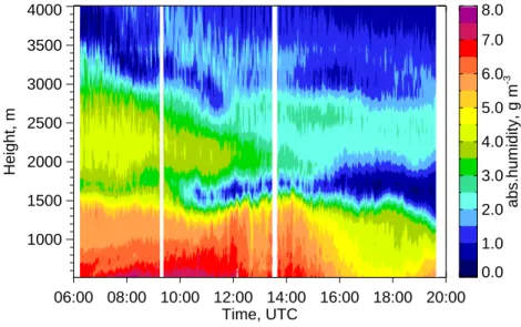
From DIAL measurements vertical profiles of absolute humidity with a time resolution of 10 s can be derived. As Fig.2shows, the humidity structure in the lower troposphere is depicted, in particular the evolution of the convective boundary layer with a marked

25

upper boundary which reaches up to 1500 m around noon. But also synoptic-scale influences like humidity advection above the CBL are shown.

ACPD

Full Screen / Esc

Printer-friendly Version

Interactive Discussion The accuracy of the derived absolute humidity values is determined by systematic

errors which are small and well assessed (B ¨osenberg, 1998) and by random errors which depend on atmospheric conditions, height, and resolution. Actual random errors are estimated for each measurement. For the ABL altitude range and typical conditions during the measurements presented here a value of<0.2 gm−3 can be assumed.

5

2.5 Surface evaporation, soil moisture

In order to obtain area-averaged surface fluxes of latent and sensible heat from the energy balance network, flux composites were derived for each surface type by aver-aging data from the different stations operated over the same type of surface. Then averages for the three main land use classes (farmland, forest, water) and a weighted

10

area-average over the whole study region were determined considering the percentage of each surface type in the area (for details, seeBeyrich et al.,2006). For this study only the composite flux values for farmland were used because this is the prevailing land use class in the corresponding model gridbox (see Sect.3). The averaging time is 30 min. The uncertainty range of composite fluxes is determined byBeyrich et al.

15

(2006) and is approximately 10% for sensible heat flux and 15–20% for latent heat flux. Soil moisture data are not averaged because the measurements at different locations differ strongly - although the trends are similar – and measurement depths differ, too. One location with continuous measurements is chosen as a proxy and the data are only compared qualitatively with model data.

20

2.6 Boundary layer height

The boundary layer height which can be clearly seen in Fig.2is derived from the DIAL offline backscatter signal. The method of Lammert and B ¨osenberg (2006) is used which is based on the analysis of average and instantaneous data by searching for the maximum in the vertical variance profile and the maximum in the gradient profile of

25

ACPD

Full Screen / Esc

Printer-friendly Version

Interactive Discussion mask (see Sect.2.8.1) into the backscatter data so that only in cloud-free regions the

ABL height is determined. The 10 s boundary layer heights are averaged over one minute.

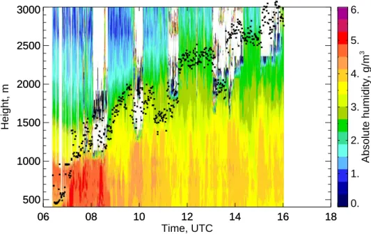
Figure 3 shows examples of days with and without boundary layer clouds to illus-trate the performance of the method. The top of the CBL is well detected, sometimes

5

there are difficulties in finding the growing CBL height in the morning. The top of the residual layer height is also detected by this method because its undulating structure also causes a maximum in the variance profile, but results are often not as clear as in Fig.3, left panel. For these reasons the comparisons with REMO will be restricted to the fully developed CBL between 10:00 and 16:00 UTC.

10

The height resolution of CBL-height is 15 m. The accuracy strongly depends on atmospheric conditions and is estimated in a cloud-free and well-defined CBL as better than 50 m, but deviations due to ill-defined ABL may be as large as 200 m (Hennemuth

and Lammert,2006).

2.7 Vertical water vapour transport

15

The water vapour flux was determined by the eddy-covariance method from fluctua-tions of humidity and vertical wind measured by synchronised DIAL and Doppler lidar, operating side by side. The measurements, which took place during the first campaign, are described byLinn ´e et al.(2006). Flux values are calculated at 30 m intervals with an averaging period of 90 min. Since wind data are only available in aerosol loaded

20

layers, the flux values are mainly restricted to the boundary layer. Figure4illustrates the availability of vertical wind and humidity fluctuation measurements and derived wa-ter vapour flux profiles at special time inwa-tervals. Depending on the mean horizontal wind speed the recorded dominating eddies may have a time scale of up to 30 min of minutes (see Fig.4, upper panels). This leads to a rather large sampling error.

25

Typical total error values for 90 min average flux values are±50 W m−2(Linn ´e et al.,

ACPD

Full Screen / Esc

Printer-friendly Version

Interactive Discussion 2.8 Cloud parameters

Scattering of millimeter waves is particularly suited to characterise cloud parameters because most clouds can on one hand be detected and on the other hand are pen-etrated, even if there are multiple optically thick cloud layers. Cloud parameters to be determined by radar are cloud cover, cloud boundaries and thickness, number of

5

layers, liquid water content and ice water content.

Main ambiguities in cloud parameter retrieval from radar reflectivity are due to the proportionality to the 6th moment of the cloud drop size distributionN(D). Thus quan-titative retrieval of liquid water content (proportional to the third moment of N(D)) is obviously impossible without assumptions on the shape ofN(D). Even the observed

10

cloud boundaries is sometimes affected by the D6-dependence of the radar echo. Particularly cloud-base detection in the boundary layer can be impaired by mainly two mechanisms:

– Clouds often release small amounts of drizzle, which evaporates at some height

between the cloud base and the surface. As drizzle drops are larger than cloud

15

drops, they tend to dominate the radar echo due to the D6-dependence, even if their liquid water content is negligible.

– During daytime in the warm season particulate echos from the cloud-free

bound-ary layer can be misinterpreted as clouds. Insects or seeds are assumed to be the main source of these echos (sometimes referred to as “atmospheric plankton”).

20

In addition, optical relevant clouds can sometimes fall below the detection threshold of the radar when cloud particles are too small. This occurs preferably in shallow convective ABL clouds (e.g. cumulus humilis) or in high cirrus clouds.

In this study only the radar reflectivity factorZ was considered, although spectral and polarimetric data with high potential to mitigate many of the mentioned shortcomings

25

ACPD

Full Screen / Esc

Printer-friendly Version

Interactive Discussion tested algorithms to exploit this information except for case studies and by the fact that

those data were not continuously available.

Optical ceilometer data, which were continuously available, provided an alternative to eliminate the cloud base ambiguities. Due to the D2-dependence of the optical returns for the given range of particle sizes drizzle and atmospheric plankton had nearly no

5

effect on optical data. Therefore ceilometer data, and if available, lidar data were used to determine the lowest cloud base in the ABL. In addition the comparison of radar and lidar data provided an estimate of the fraction of high cirrus clouds below the radar detection threshold. The ratio of clouds detected only by lidar and clouds detected by radar and lidar is 2.7 for the height range of 9 km to 12 km. This underlines the

10

necessity of using an additional optical instrument for cloud detection particularly for heights above approximately 10 km.

Cloud base determination with ceilometer relies completely on the proprietary algo-rithm of the system manufacturer. According to C. Muenkel (private communication) the algorithm first identifies rain sections in the lowest 2000 m of the range- and

overlap-15

corrected signal profile by checking signal strength and height range threshold values. Clouds can be detected within and outside rain sections by either checking the slope steepness or signal strength, and cloud base height is set to 15 m below the height of the maximimum signal within the cloud peak.

In about 30% of times the offline channel of the DIAL was used for cloud detection

20

with very high sensitivity. Only signals with a signal-to-noise-ratio SNR>5 are used, and cloud boundary detection is based on the analysis of the small scale variances (40 ms/15 m resolution). Since backscatter shows a sharp increase at cloud bound-aries and the edges are variable in time and height, the shot-to-shot signal variance shows a pronounced maximum at the cloud boundaries. Signal strength is used

addi-25

tionally to select only those variance maxima associated with clouds.

Different cloud detection algorithms exist, based on the maximum in the backscatter coefficient profile (Hogan et al.,2003) or on a wavelet analysis (Haeffelin et al.,2005), used at the SIRTA site (France). A systematic algorithm comparison was beyond the

ACPD

Full Screen / Esc

Printer-friendly Version

Interactive Discussion scope of this study.

2.8.1 Cloud morphology

Vertical profiles of cloud boundaries were evaluated with a resolution of ∆t=1 min, ∆z=30 m. The automatic detection of clouds with radar requires the knowledge of the noise levelP_n at the radar receiver input. In this study P_n was obtained from the

5

receiver signal, measured after the transmit pulse with a delay corresponding to 12 km height. It is assumed that no echo is received from that height, and that the mean noise power does not change with delay time. With knowledge ofP_n and of the number of incoherent averages a cloud mask consisting of 5 pixels in range and 5 pixels in time, as described byClothiaux et al.(1995), was established.

10

Figure 5 gives an example of a time-height section of the radar reflectivity and the Doppler velocity. It can be seen that multiple cloud layers are penetrated by the radar. The echos from particles inside the ABL, which have to be masked with lidar data, are clearly visible. Rain events can be detected by the Doppler velocity as shown in Fig.5, lower panel.

15

Figure6shows an example of the range-corrected backscatter signal – original and with cloud mask – of the offline channel of the DIAL and the lidar-derived cloud mask for one day.

The complete cloud mask is then derived from the combination of both instruments by using lidar data for lowest cloud base height, radar data for cloud top heights and

20

cloud base heights above water cloud layers. This method was also applied byIntrieri

et al. (2002).

Figure7shows the radar-lidar cloud mask. It can be seen that the lidar beam cannot penetrate water clouds because the signal is rapidly attenuated by strong scattering from water droplets. High cirrus clouds and some low-level small-particle clouds on the

25

other hand are invisible for the cloud radar. Elevated cloud base heights agree well for both instruments.

ACPD

Full Screen / Esc

Printer-friendly Version

Interactive Discussion depend on the height of the cloud bases and tops. High cirrus clouds above 10 km

are only visible for the lidar (see Sect.2.8). But lidar measurements are only available at 33% of all radar measurements and even in those periods the lidar beam is often blocked by low-level water clouds.

The rms-deviation of cloud base height as determined by the two lidar systems,

5

DIAL and ceilometer, is about 100 m and characterises the uncertainty caused by the different retrieval algorithms. The error in the cloud base height determination by cloud radar is as small as the height resolution, i.e. 30 m, but the cloud base may be not well defined The cloud cover, which was derived from these observations, is defined in Sect.4.3.

10

2.8.2 Water content of clouds

The key parameter describing the role of clouds in the water cycle is – besides the geometrical size – their water content which is denoted here byM. It is determined by: M = π

6 ρ Z∞

0

N(D)D3d D (1)

whereD is the dropsize, N(D) is the dropsize distribution and ρ is the water density.

15

Unfortunately,N(D) cannot be measured directly because Z =

Z∞ 0

N(D)D6d D (2)

Therefore M is estimated from the Ka-Band radar measurements by using empirical Z–M relations of the form:

Z = a Mb (3)

20

wherea and b are empirical constants.

These Z-M relations were obtained from the independent determination of liquid water content (LWC) and radar reflectivity of known dropsize distributions. Dropsize

ACPD

Full Screen / Esc

Printer-friendly Version

Interactive Discussion distributions can be obtained from airborne probes, cloud physical model calculations

or the combination of remote sensing instruments (see e.g., Sauvageot and Omar,

1987).

A large problem deriving cloud water content is imposed by drizzle within water clouds. New attempts to take this effect into account use different Z-M relations for

5

clouds without drizzle, with a slight drizzle portion and with a large drizzle portion (see Fig. 8). According to a suggestion of Krasnov and Russchenberg (2003) these rela-tions hold for certain dBZ-ranges which are also used in this study. For dBZ< − 30 the relation of Fox and Illingworth (1997), for −30<dBZ<−20 the relation of Baedi et al.

(2000), and for dBZ>−20 the relation ofKrasnov and Russchenberg(2002) is applied.

10

There exist a variety of algorithms to derive LWC from cloud radar data which differ mostly in the coefficients in Eq. (3). Advanced methods combine instruments like cloud radar, microwave radiometer and radiosonde or make use of multi-wavelength radar systemes (see e.g.,Meywerk et al.,2005;L ¨ohnert et al.,2004;Gaussiat et al.,2003).

Krasnov and Russchenberg(2006) suggested the use of lidar-derived optical extinction

15

to determine the optimum choice of parametersa and b in Eq.3.

The ice water content of clouds (IWC) can be similarly calculated from aZ-M relation (e.g.,Sassen,1987;Liu and Illingworth,2000) with M denoting IWC here. But since dif-ferent ice crystal types which can be assigned to certain height - and thus temperature – ranges cause different reflectivity, a new Z–M relation was suggested byHogan et al.

20

(2006). This algorithm stratifies theZ-M relation with temperature and is illustrated in

Fig.9. Hogan et al.(2006) derive two different formulae for different aims, one formula

seems to give best results for the expected value of IWC when compared with aircraft measurements (black lines), the other formula gives better agreement when comparing variances or PDFs of IWC (red lines).

25

Generally, the derivation of cloud water content from radar reflectivity suffers from several simplifying assumptions. Better algorithms to discriminate between water droplets and ice crystals make use of the reflectivity ratio of the radar and lidar sys-tems (Tinel et al.,2005). In this study this method was not applied because of the low

ACPD

Full Screen / Esc

Printer-friendly Version

Interactive Discussion lidar availability particularly at high levels.

The accuracy of cloud radar-derived liquid water content and ice water content using Z-M relations is nearly entirely determined by the validity of the assumptions of the applied methods. The liquid water determination only from reflectivity may - according to the situation – enclose large errors up to±10 dBM.

5

2.9 Precipitation

Precipitation measurements are continuously available from the PLUVIO network and from one MRR at Lindenberg. The general difficulty that point measurements are not necessarily representing the average inside a model grid box applies particularly to precipitation due to the extreme spatial heterogeneity of the precipitation field. In this

10

study the network data are used for calculating area averages of rain rates, while the MRR data represent a single station. The results differ both in rain sum and in time structure (see below Fig.25). The reason is that precipitation is strongly heterogeneous as e.g. shown for the measurement period in 2003 byBeyrich and Mengelkamp(2006). The MRR rain rates are nearly always smaller than those of the network. MRR point

15

measurements have earlier been compared with a conventional rain gauge aside, and the 30 min averages deviate by approximately 20% (Peters et al.,2002).

3 Regional model REMO

The regional climate model REMO is a hydrostatic, three-dimensional atmospheric model, that has been developed in the context of the Baltic Sea Experiment

(BAL-20

TEX) at the Max-Planck-Institute for Meteorology in Hamburg, Germany. It is based on the Europa Model, the former numerical weather prediction model of the German Weather Service and is described inJacob (2001) and Jacob et al. (2001). REMO uses the physical package of the global circulation model ECHAM4 (Roeckner et al.,

1996;DKRZ,1994) and can be run in forecast as well as in climate mode. Prognostic

ACPD

Full Screen / Esc

Printer-friendly Version

Interactive Discussion variables are the horizontal wind components, surface pressure, temperature, mixing

ratio of water vapour and of cloud water.

The surface fluxes are determined by a bulk equation taking into account the differ-ence of momentum, energy or water vapour at the surface and at the lowest model level. The transfer coefficient consists of a neutral part and a stability function after

5

Louis (1979). Surface evapotranspiration is composed of evaporation from the skin

reservoir, bare soil, vegetation and snow (DKRZ, 1994). Soil moisture is – in con-trast to soil temperature – determined at only one layer by a budget equation which includes evaporation, rainfall, surface runoff, drainage and snow melt (D ¨umenil and

Todini,1992). This type of scheme is called a “bucket model”.

10

The vertical turbulent transport in the atmosphere is parameterised by a local diffu-sion equation. The diffudiffu-sion coefficient is the product of the square root of the turbulent kinetic energy (TKE) and a length scale which is a prescribed length scale times a stability function. For TKE a prognostic equation is solved (“TKE-closure”). In the dry atmosphere no entrainment scheme is included. In this study the instantaneous latent

15

heat flux in the atmosphere is recalculated from the diffusion coefficient and humidity profiles.

The height of the atmospheric boundary layer can be diagnosed from model output parameters or can be taken from the diffusion subroutine. This parameter is determined as the maximum value of two parameters,

20

hbl = max(hdyn, hcnv), (4)

the dynamical height hdyn = 0.5

u_∗

f (5)

withu_∗: friction velocity and f : Coriolis parameter and the convective height which is the height of the lowest level with a static stability larger than at the first level (DKRZ,

25

ACPD

Full Screen / Esc

Printer-friendly Version

Interactive Discussion boundary layer hcnv can also be determined as the height where the gradient of

po-tential temperature or of absolute humidity or of TKE is largest. These methods refer to the definition of the CBL as a turbulent well-mixed layer with an inversion on top which restricts transport of matter to the CBL, see e.g. the discussion inHennemuth

and Lammert (2006). The CBL height values from different definitions mostly agree on

5

undisturbed days with strong insolation while they may differ much on non-ideal days (see below, Fig.17).

The simulation of clouds and precipitation in REMO is divided into the stratiform cloud and precipitation scheme accounting for clouds developing on scales that can be described directly by the prognostic variables of the model, and in the convective cloud

10

and precipitation scheme for clouds on smaller scales. The stratiform cloud scheme in REMO, taken from the MPI Global Model ECHAM4, is based on the approach of

Sundqvist (1978) and is described in detail in (DKRZ, 1994) and in Roeckner et al.

(1996). In-cloud waterqc is diagnosed assuming that the predicted cloud water mixing ratioq_w is confined to the cloudy part of the gridbox. q_c is then split into cloud ice

15

water content (IWC) and cloud liquid water content (LWC) as a function of temperature followingRockel et al.(1991) (Fig.10): above the melting point – here 0◦C – the cloud consists entirely of liquid water while near -50◦C the cloud almost entirely consists of ice.

Convective clouds in REMO are parameterised using the Tiedtke mass flux scheme

20

(Tiedtke,1989) with some modifications followingNordeng(1994).

Total precipitation in REMO is the sum of precipitation formed in the stratiform cloud scheme and precipitation formed in the convective cloud scheme. Cloud cover is cal-culated as a nonlinear function of the grid-mean relative humidity.

ACPD

Full Screen / Esc

Printer-friendly Version

Interactive Discussion

4 Quality assessment experiment

4.1 Site and time table

The Meteorological Observatory Lindenberg of the German Weather Service (DWD) is located 60 km southeast of Berlin (Neisser et al.,2002). The terrain is flat with gently rolling hills of less than 50 m, and its hetereogeneous landscape of agriculture, forests,

5

small lakes and villages is typical for the region and also for northern Central Europe. The measurements took place in three time periods, 20 May 2003 to 14 June 2003, 11 May 2004 to 6 June 2004, and 26 August 2004 to 30 September 2004. The first campaign was the LITFASS-2003 campaign within the EVA GRIPS project of the Ger-man Climate Research Program (DEKLIM) (Beyrich and Mengelkamp,2006) aiming at

10

the determination of area-averaged surface evaporation over a heterogeneous surface. LITFASS stands for Lindenberg Inhomogeneous Terrain – Fluxes between Atmosphere and Surface: a Long-term Study)

The comprehensive instrumentation at MOL, set up in order to characterise the ver-tical structure of the atmosphere includes energy balance stations (enhanced number

15

during LITFASS-2003), a network of rain gauges, a ceilometer, a microwave cloud radar, and a Micro Rain Radar. Additional instruments during the three campaigns were a Differential Absorption Lidar (DIAL) and a Doppler lidar (operated by MPI for Meteorology).

Comparisons are performed for all three measuring periods. Only in case of a

re-20

stricted availability of special data the period is shortened. 4.2 Model runs

In this study REMO was run in the forecast mode in order to simulate the atmospheric conditions at Lindenberg as close to the real weather as possible. This means that the model was initialized at 00:00 UTC and the forecast times from 07:00 UTC of the

25

ACPD

Full Screen / Esc

Printer-friendly Version

Interactive Discussion 1/6◦, i.e. approximately 18 km. The model runs were nested in 1/2◦ runs which were

initialized and driven at the boundaries with ECMWF analyses. Figure11 shows the model domain of the 1/2◦runs and of the nested 1/6◦runs.

The water cycle parameters which are compared with observations are absolute humidity (calculated from mixing ratio and temperature), surface latent heat flux, soil

5

wetness, water vapour transport in the atmosphere, cloud cover, cloud liquid water content, and precipitation. Output parameters are available every 1 h. Two different models levels are distinguished, full levels which characterise the centre of gravity of the model layers as well as half-levels which are the boundaries of the model layers. The model levels are transformed to pressure levels by means of the surface pressure

10

value, and then the individual height of these levels is calculated using the barometric height equation. The predicted values are defined on full levels, for the comparison with observations they are regarded representative for the layer between the adjacent half levels.

4.3 Transformation of observational data to model grid

15

All vertical profiles of water cycle parameters - absolute humidity, cloud cover, cloud liq-uid water content and cloud ice water content – are transformed to the vertical grid of the model REMO with ∆z≈35 m near the surface and ∆z≈1600 m at 10 km. For vertical averaging the time-dependent REMO level heights are averaged over all model runs. The observational data are then averaged for the layers between the half levels. The

20

measured humidity values are averaged over±10 min around the model output times and are compared with instantaneous model values. The boundary layer height is av-eraged over±15 min around the model output times because the values are strongly variable. Surface fluxes are averaged over 1 h, precipitation is added up to 1 h. The observed cloud cover is the percentage of cloud signals detected in height/time boxes

25

with vertical extension equal to the respective REMO layer thickness and with 1 h du-ration corresponding to the REMO output time interval Only data with more than 2% cloud cover are regarded as clouds. Cloud LWC and IWC are averaged over height

ACPD

Full Screen / Esc

Printer-friendly Version

Interactive Discussion and time of REMO grid boxes.

4.4 Representativeness and comparability of data sets

The two data sets of water cycle parameters – derived from observations and the model – differ in spatial and temporal representativity. Therefore, the comparability and its limitations should briefly be discussed.

5

Model parameters are partly instananeous values (humidity, cloud water content, soil wetness, and parameters derived from instantaneous parameters like cloud cover, soil wetness and atmospheric fluxes) and partly means or sums over 1 h (surface evapora-tion, precipitation). If possible, instantaneous values are compared to observations of short averaging time (humidity, ABL height, see Sect.4.3).

10

Simulated values are representative for the grid box or surface area defined by the horizontal model resolution. Additionally, the numeric calculation scheme introduces an uncertainty of one mesh size in each direction. The uncertainty can be estimated by the difference of neighbouring values to the selected gridbox and can be regarded as negligible in a rather uniform area like the Lindenberg area. Thus a height uncertainty

15

of one vertical mesh size remains.

The accuracy of measurement-derived water cycle parameters is given in Sect. 2, but additional uncertainties arise from the transformation to the model grid. Height av-eraging over increasing intervals with increasing height and time avering over 1 h or shorter intervals smoothes small-scale features and thus improves the comparability

20

with model values which are representative for a 300 km2gridbox. But averaging may in the case of cloud cover lead to a larger portion of small cloud cover values. Generally, time averages of point measurements are compared with area-representative model values. Under the assumption of Taylor’s hypothesis in a divergence-free flow, time averaging approaches spatial averaging. For surface values the use of area-averaged

25

observations – e.g. from networks – is highly recommended because surface hetero-geneities are mostly large (Mengelkamp et al.,2006). Atmospheric heterogeneities are assumed to be smaller because of atmospheric mixing (Parlange et al.,1995).

ACPD

Full Screen / Esc

Printer-friendly Version

Interactive Discussion There exists a general problem in comparing observed and modelled clouds

be-cause the parameters are derived differently. Cloud boundaries and cloud cover are derived directly from measured radar and lidar reflectivity, but cloud liquid water and ice water content are diagnosed making certain assumptions. The opposite is the case for models, here total water content – in enhanced models liquid water content and ice

5

water content – is predicted, but cloud cover is diagnosed from the predicted relative humidity. So in the comparison of cloud cover and liquid/ice water content one of the respective parameters is diagnosed using assumptions which may not be valid for all situations. This has to be kept in mind in the discussion of comparisons.

5 Results of comparison

10

5.1 Humidity field, evaporation, soil moisture

The direct comparison of simulated and observed humidity fields in the lower tropo-sphere shows that the evolution of the CBL is well reproduced in the model, although height of the boundary layer and humidity values do not always agree with observa-tions.

15

For a statistical analysis the observed humidity field transformed to the REMO grid is used. The number of data pairs per gridbox – i.e. the number of observations – is shown in Fig.12. The boundary layer is best represented below 1500 m and between 07:00 and 18:00 UTC, in the region above the boundary layer less observations are available because of cloud occurrences and limited range of the DIAL used in 2004.

20

Statistical analysis is performed for 1 h-intervals with observations. Simulated and observed humidity values are well correlated within the convective boundary layer be-low 1000 m and in the be-lower part of the free atmosphere (around 2000 m) as Fig.13, upper panel shows. In the lower height levels the correlation coefficient is larger than 0.75, whereas in the layer between 1000 m and 2000 m the correlation coefficient is

25

ACPD

Full Screen / Esc

Printer-friendly Version

Interactive Discussion lie above the CBL, as this is often too low in the model (see Sect. 5.2). A marked

distinction between the layer below 1000 m and the layer between 1000 m and 2000 m is also reflected in the bias and the rms-error (Fig.13, middle and lower panel). While the humidity below 1000 m is strongly biased (“model – observation”: 1.5 to 3 g m−3) but exhibits a low rms-error, the humidity above the CBL agrees well on average, but

5

shows a large rms-error.

This difference is also manifest in statistics of humidity values from all grid boxes in the range of 500 m to 1000 m and 1000 m to 2000 m. Data between 10:00 to 16:00 UTC are taken into account. Figure14shows the related scatter plots.

The statistical results are presented in Table3. The data in the lower range, i.e. in

10

the CBL, are well correlated but are strongly biased. Whereas the data in the layer where the model often predicts free atmosphere show a large scatter, which results in a poor correlation and enhanced rms-error. The errors lie far beyond the measurement uncertainty.

The analyses suggest that in most cases the simulated boundary layer is too low and

15

too moist. One crucial parameter determining the humidity field in the boundary layer is evaporation. During LITFASS-2003 there was the opportunity to compare REMO evaporation with an areal average of evaporation from a network of micrometeorologi-cal stations. Figure15shows time series of simulated and observed surface fluxes for a 12 day period.

20

The simulated latent heat flux is much larger than the observed one, the sensible heat flux is lower. There are only a few days on which the modelled latent heat flux is equal to or even smaller than the observed flux on 27 May, 31 May, 6 June, and 9 June. These are days with or after rain events with the consequence of a decreasing Bowen ratio. The deviations between modelled and measured fluxes is – at least for the latent

25

heat flux – much larger than the measurement uncertainty of maximum 20% stated in Sect.2.5, the agreement on wet days is within this range.

Since boundary layer processes are influenced by soil parameters we compare mod-elled and observed soil moisture. A direct comparison of simulated and observed soil

ACPD

Full Screen / Esc

Printer-friendly Version

Interactive Discussion moisture is difficult because REMO has a one layer scheme and the measurements

comprise several soil layers. The measured soil moisture is given in volume percent-age and the simulated soil moisture is soil water content in m. So the time series are only being compared qualitatively here. Figure16shows the evolution of observed and simulated soil moisture during LITFASS-2003. It is obvious that during dry periods the

5

soil moisture decreases steadily in all depths, and after rain events the upper layers are moistened. The simple “bucket”-model of REMO shows decreasing soil wetness and only little reaction to rain events. The large increase in soil moisture in the upper 10 cm which dominates evapotranspiration cannot be simulated by the one layer scheme. The deviation between observation and simulation relates to the missing vertical structure

10

of soil moisture. Error ranges cannot be supplied. 5.2 Boundary layer height

The structure of humidity profiles in the lower troposphere is closely related to the ABL depth. In high-pressure situations it is controlled by the sensible heat flux at the sur-face, the stratification of the free atmosphere, and synoptic-scale subsidence (see e.g.,

15

Batchvarova and Gryning,1994). From REMO simulations four ABL height values can

be derived according to different definitions (see Sect.3). They are compared with ABL heights derived from DIAL measurements. Figure17shows two examples of the time development of the ABL height. On 10 June 2003 the coincidence between all mod-elled and the observed ABL height is good although the observed maximum height of

20

the CBL is approximately 500 m larger than the simulated height. The underestimation of the CBL height by REMO is more obvious on 7 June 2004. The latter example is from a day with boundary layer clouds and shows that the variability of the ABL height is large. The representation of boundary layer clouds in REMO will be discussed later in Sect.5.4.

25

Leaving out all days with a complex development like frontal passage, strong ad-vective influences or breakdown of ABL height and regarding only the values between 10 and 16:00 UTC the scatterplots between the observed ABL height with the

differ-ACPD

Full Screen / Esc

Printer-friendly Version

Interactive Discussion ent REMO ABL heights show large deviations (Fig.18shows the ABL height derived

from the parcel method). The correlation coefficient between observed and different model-derived ABL heights is in the range of 0.28 (for the potential temperature gradi-ent method) to 0.50 (for the parcel method). The observed ABL height covers a larger range of height values compared to the model ABL height. Even if an error of observed

5

ABL height of 200 m and additionally the REMO height uncertainty of 160 m at 1000 m height is assumed it is obvious that most deviations are larger.

The lower panel of Fig.18 shows the same relation, but only for undisturbed days after rain events. The agreement is much better, the correlation coefficient varies be-tween 0.43 (for the TKE gradient method) and 0.81 (for the humidity gradient method

10

and the parcel method). This confirms the ability of the model to well simulate situations with wet soils.

5.3 Vertical water vapour transport

Within the convective boundary layer water vapour is transported vertically by turbu-lent and convective eddies. The surface is generally a source of water vapour and

15

evaporation increases the water vapour amout in the boundary layer. Entrainment of air from the free atmosphere into the boundary layer occurs during the growth of the CBL (Stull,1988). This is in most cases a downward flux of dry air. In situations with moist air advected over the ABL or with the CBL growing in the humid residual layer the entrainment flux may also be near zero. The top-down and bottom-up processes

20

control the humidity profiles in structure and amount (Mahrt,1976).

The measured and simulated flux profiles are only compared qualitatively, because the surface values differ a lot (see Sect.5.1). The simulations mostly show a large pos-itive entrainment flux in the morning connected with the CBL growth and after reaching a nearly constant CBL height either a slightly increasing or a slightly decreasing flux

25

profile with height. The flux magnitude is determined by the surface flux. Details of the profiles should be looked at with caution bearing in mind that the model flux is re-calculated with instantaneous output values while the observed flux is a time average

ACPD

Full Screen / Esc

Printer-friendly Version

Interactive Discussion over turbulent fluctuations.

Figure19shows latent heat flux profiles for two days with different characterics. On 30 May 2003 a large entrainment flux is observed during the period of growing CBL. On 9 June 2003 the flux is nearly constant with height in the CBL and decreases at its top. This general structure remains even when accounting for the accuracy of the

5

observations which is about±50 W m−2. The simulated flux profiles also show these features: increasing flux with height on 30 May and slightly decreasing flux with height on 9 June. But since the environmental conditions differ there are also differences in water vapour transport. On 30 June the CBL is steadily growing with large entrainment of dry air. The model CBL remains shallow and the entrainment stops after reaching

10

the final height extent. On 9 June no entrainment flux is observed in the morning because the residual layer is humid, but the simulations show a large entrainment of dry air in the morning.

Generally, the observed profiles of latent heat flux often exhibit a decrease with height in the lower part of the CBL and – in case of entrainment of dry air – an

in-15

crease towards the top of the CBL. This tendency cannot be found in simulated flux profiles which steadily increase or decrease with height throughout the CBL.

5.4 Cloud amount

Simulated and observed clouds are compared in a two-fold way, the occurrence of a cloud in the gridbox is considered as well as the cloud cover. Figure20 shows cloud

20

cover on three days with clouds in several layers. The first impression is that the model predicts too few clouds at all levels except above 10 km height, and that the predicted cloud cover is mostly less than the observed one.

For a statistical analysis the number of cloud occurrences is counted for each height level and the cloud cover is added up. The results are shown in Fig.21. Both

obser-25

vations and simulations show two maxima of cloud occurrence and cloud cover, one maximum around 2000 m and a second maximum between 9000 m and 11 000 m. The mid-level region around 5000 m exhibits a distinct minimum of clouds. This structure

ACPD

Full Screen / Esc

Printer-friendly Version

Interactive Discussion of cloud occurrence is typical for mid-European climate and reported by e.g. Hogan

et al. (2001),Brooks et al.(2004),Will ´en et al.(2005). It is obvious that in most height levels nearly twice as many clouds are observed than simulated. The same is true for the cloud cover sum. The opposite tendency can be seen for high-level clouds. Above 11 km the same number of clouds is observed and modelled, but the corresponding

5

cloud cover is smaller in observations than in the model. Similar results are found in other sudies, e.g. for Europe byHogan et al.(2001) and bySengupta et al.(2004) for the ARM site in the southern Great Plains (USA).

The cloud observations, mainly based on cloud radar data, may still contain some non-cloud echos (compare Sect. 2.8). Most of these remaining echos are blinded

10

when transforming the cloud mask to the grid where only averages larger than 2% are retained (see Sect.4.3). Excluding all cloud observations with cloud cover smaller than 0.2 yields a better agreement with the number of simulated clouds at low and mid levels. But the tendency of the model to underestimate the number of low-level and mid-level clouds remains. As discussed in Sect. 4.4the quantity cloud cover is determined in

15

different ways from modelled and observed values – with cloud cover being directly derived from observations – and obviously the results differ strongly. For high-level clouds above 10 km the observational data are not of sufficient reliability to assess the quality of model cloud data (compare Sect.2.8). The observed cloud amount is biased and a quantitative comparison is not possible.

20

An analysis of observed and simulated clouds for different times of the day and heights is shown in Table4. Here we regard all cloud observations. Cloud occurrence and cloud cover are counted for cloud levels 0 m to 3000 m (low), 3000 m to 6000 m (mid), and >6000 m (high) and for time periods 04:00 UTC to 09:00 UTC (morning), 10:00 UTC to 15:00 UTC (noon), 16:00 UTC to 21:00 UTC (evening), and 22:00 UTC

25

to 03:00 UTC (night).

The Table shows that REMO predicts too few clouds at all times and heights with one exception of night-time high-level clouds. Generally, the agreement is best at night and for high-level clouds. The largest differences between observed and simulated cloud

ACPD

Full Screen / Esc

Printer-friendly Version

Interactive Discussion occurrence are found for low-level clouds in the morning and around noon. This kind

of cloud is typically fair-weather convective boundary layer cloud. The sum over cloud cover confirms these results.

The observations show that boundary layer clouds extend over several grid levels whereas model ABL clouds are often restricted to one, two or three layers. Moreover,

5

simulated boundary layer cloud bases are lower than observed ones. This is illustrated by Fig.22for 7 June 2004. For this day a comparison of ABL height is shown in Fig.17. It is clear from this figure that there is a broad entrainment layer of several 100 m with scattered clouds. This is also evident from Fig.17. The model does not show such a broad cloud layer. The height of the average maximum of cloud occurrence is 1760 m

10

for observed clouds and 1380 m for simulated clouds. The peak width at half-height to the upper minimum is 1500 m for observed, and 900 m for simulated clouds.

While cloud amount and cloud cover differ between observations and simulations the number of cloud levels is quite similar (Table5). There is a tendency for REMO to produce slightly more cloud levels than observed. This is particularly the case when

15

compact clouds are observed which extend over nearly the whole troposphere and the model separates the cloud into several layers (see Fig.20, lower panels).

5.5 Water content of clouds

The total cloud water content of clouds consists of liquid water and ice water. Over a wide temperature range the clouds contain both droplets and ice crystals which is

20

expressed in the model by the function determining the portions of LWC and IWC by temperature (see Fig. 10). But the determination of LWC and IWC in mixed clouds from radar reflectivity demands the partitioning of the reflectivity which is a difficult task requiring the solution of not well established empirical non-linear equations. So for this study only those clouds are compared for which the assumption of mainly water clouds

25

or mainly ice clouds holds. This is determined by use of the REMO temperature values. Water clouds are supposed to occur below 3000 m where on most days temperature is above 2◦C. Only cloud radar data which are masked by ceilometer data are used. But

ACPD

Full Screen / Esc

Printer-friendly Version

Interactive Discussion additionally, the lower region up to 1800 m is excluded because of the problems with

remaining non-cloud echos in radar reflectivity. The number of observed clouds in this layer is 2760, the number of simulated clouds only 790 because many of the model ABL clouds appear below 2000 m. Ice clouds are assumed to be in the region above 7000 m where temperature values below –30◦C prevail. According to the temperature

5

– IWC relation (Fig. 10) only less than 7% of the cloud water is liquid water. The number of model ice clouds for the comparison is 545 while the number of observed ice clouds is 683. For both regions the observation-derived LWC and IWC, respectively, are compared with REMO total cloud water.

Liquid water content

10

Figure23shows the frequency distributions of simulated and observation-derived LWC in supposedly water clouds. The distribution of simulated LWC has a peak between 10−1 and 10−2g m−3 and there are no values larger than approximately 0.25 g m−3. Values smaller than 10−3g m−3occur rarely.

The frequency distribution of LWC from cloud radar data covers the range between

15

10−3and 1 g m−3 with a nearly constant frequency between 10−3 and 10−1g m−3 with a maximum near 1 g m−3. This peak is probably an artefact of the cloud radar data due to the inadequate treatment of drizzle droplets in the clouds. We also find a cut-off of values smaller than 10−3g m−3 which may be due to the noise characteristics of the cloud radar (see Fig.1).

20

The superimposition of an artificial peak and the cut-off at small LWC values falsifies the LWC distribution and makes the accurate quality assessment of model LWC impos-sible. As mentioned in Sect.2.8.2 the LWC derived from cloud radar data is afflicted with problems and obviously the results are not plausible. Another reason for the the poor quality of the radar retrieval of LWC may be related to the systematic difference

25

(although depending on the cloud type) between radar observations of reflectivity fac-tor Z and the aircraft/balloon predictions of the same quantity, which was reported by

ACPD

Full Screen / Esc

Printer-friendly Version

Interactive Discussion Ice water content

The agreement of frequency distributions of IWC derived from the model and the cloud radar is better (Fig. 24). The radar-derived IWC is calculated according to the two algorithms given by Hogan et al.(2006) (see Fig.9) and marked in Fig. 24by “radar e” for best obtaining the expected value and “radar v” for best obtaining the variance.

5

The distributions cover the IWC range between 10−7 and 10−2g m−3with a maximum around 10−4g m−3and negative skewness. The REMO IWC distribution exhibits a nar-rower shape, it agrees with the radar IWC at large IWC values, the maximum is situated between 10−4 and 10−3g m−3, but small IWC (<10−6g m−3) values are missing. This is also evident in similar comparisons – with the mesoscale version of the Met Office

10

Unified model – in the moderate temperature range of –15◦C to –30◦C shown byHogan

et al. (2006). A reason for the missing small model IWC values may be the threshold of 80% relative humidity in the gridbox for the formation of clouds. A lower threshold value would probably favorite a larger amount of small IWC.

In this particular comparison the model IWC distribution fits better with the IWC

dis-15

tribution of “radar e” than of “radar v” for large IWC values. 5.6 Precipitation

Precipitation is the parameter with the largest spatial and temporal heterogeneity and therefore difficult to compare for one gridbox and time periods of weeks. One of the three measuring periods – LITFASS-2003 period – was exceptionally dry and is

there-20

fore excluded in this comparison. Fig.25 shows time series of rainrates for the two campaigns of 2004 determined fron the Micro Rain Radar, a network of conventional rain gauges and from REMO. The precipitation predicted by the model captures most of the observed rain events in the Lindenberg gridbox, but some events are either not simulated or not observed. The total rain sums over the two periods in 2004 which are

25

listed in Table6shows a rather good agreement of simulated and observed rain. The sum lies within the measurement uncertainty of 20% and within a certainly larger error