Dense, sonar-based reconstruction of underwater scenes

Dense, Sonar-based Reconstruction of Underwater Scenes

OFfTECHNOLOGY _by

SEP

19

2019

Pedro Nuno Vaz Teixeira

Submitted to the Department of Mechanical Engineering

LIBRARIES

in partial fulfillment of the requirements for the degree of

ARCHIVES

at the

MASSACHUSETTS INSTITUTE OF TECHNOLOGY

and

WOODS HOLE OCEANOGRAPHIC INSTITUTION

September 2019

©Pedro

Nuno Vaz Teixeira, MMXIX. All rights reserved.

The author hereby grants to MIT and WHOI permission to reproduce and to

distribute publicly paper and electronic copies of this thesis document in whole

or in part in any medium now known or hereafter created.

Author

...

Signature redacted

Department of Mechanical Engineering

August 20, 2019

Certified by

...

Signature redacted

John

J.

Leonard

Samuel C. Collins Professor of Mechanical and Ocean Engineering

Thesis Supervisor

A ccepted by ...

Signature redacted

David Ralston

Associate Scientist with Tenure, Applied Ocean Physics and Engineering

Chair, Joint Committee for Applied Ocean Science

nineeringDepartment

oGraduate Theses

Accepted by

...

Signatureredacted

Nicho as adjiconstantinou

Professbr of Mechanical Engineering

Chair, Mechanical Engineering Department Committee on Graduate Theses

Dense, Sonar-based Reconstruction of Underwater Scenes

by

Pedro Nuno Vaz Teixeira

Submitted to the Department of Mechanical Engineering on August 20, 2019, in partial fulfillment of the

requirements for the degree of Doctor of Philosophy

Abstract

Three-dimensional maps of underwater scenes are critical to-or the desired end product of-many applications, spanning a spectrum of spatial scales. Examples range from in-spection of subsea infrastructure to hydrographic surveys of coastlines. Depending on the end use, maps will have different accuracy requirements. The accuracy of a mapping plat-form depends mainly on the individual accuracies of (i) its pose estimate in some global frame, (ii) the estimates of offsets between mapping sensors and platform, and (iii) the accuracy of the mapping sensor measurements. Typically, surface-based surveying plat-forms will employ highly accurate positioning sensors-e.g. a combination of differential global navigation satellite system (GNSS) receiver with an accurate attitude and heading reference system-to instrument the pose of a mapping sensor such as a multibeam sonar.

For underwater platforms, the rapid attenuation of electromagnetic signals in water precludes the use of GNSS receivers at any meaningful depth. Acoustic positioning sys-tems, the underwater analogues to GNSS, are limited to small survey areas and free of ob-stacles that may result in undesirable acoustic effects such as multi-path propagation and reverberation. Save for a few exceptions, the accuracy and update rate of these systems is significantly lower than that of differential GNSS. This performance reduction shifts the accuracy burden to inertial navigation systems (INS), often aided by Doppler velocity logs. Still, the pose estimates of an aided INS will incur in unbounded drift growth over time, often necessitating the use of techniques such as simultaneous localization and mapping (SLAM) to leverage local features to bound the uncertainty in the position estimate.

The contributions presented in this dissertation aim at improving the accuracy of maps of underwater scenes produced from multibeam sonar data. First, we propose robust methods to process and segment sonar data to obtain accurate range measurements in the presence of noise, sensor artifacts, and outliers. Second, we propose a volumetric, submap-based SLAM technique that can successfully leverage map information to correct for drift in the mapping platform's pose estimate. Third, and informed by the previous two contributions, we propose a dense approach to the sonar-based reconstruction prob-lem, in which the pose estimation, sonar segmentation and model optimization problems are tackled simultaneously under the unified framework of factor graphs. This stands in contrast with the traditional approach where the sensor processing and segmentation, pose estimation, and model reconstruction problems are solved independently. Finally, we pro-vide experimental results obtained over several deployments of a commercial inspection platform that validate the proposed techniques.

Thesis Supervisor: John

J.

Title: Samuel C. Collins Professor of Mechanical and Ocean Engineering

Acknowledgements

I would first like to thank Prof. Franz Hover for accepting me into the Joint Program, and for his mentorship and advice, which was certainly fundamental in successfully nav-igating the first years of graduate school. Over classes and lunches, research and trips, experiments and long conversations, Brooks, Chris, Eric, Josh, Lucille, and Mei made for great colleagues and friends.

I am also very grateful to Prof. John Leonard for taking me into the Marine Robotics

group while simultaneously handling his sabbatical leave. At the Marine Robotics group

I have learned tremendously and gained great insight from the discussions and

conver-sations with people in the group. I am particularly grateful to Brendan, David, Kevin, Kurran, Mark, Ross, Roxana, Sudeep, and Tonio.

Between "showing me the ropes" on the first HAUV experiments and the many re-search discussions over the phone, Prof. Michael Kaess has been a steadfast source of advice and support over the years, for which I am truly thankful. Prof. Hanu Singh's knowledge and expertise have been very valuable, and the occasional field story has made many classes and meetings much more captivating and entertaining. I have also been for-tunate for the opportunity to spend a Summer at Prof. Erin Fischell's lab at WHOI, and to witness her talent and enthusiasm. She has been a very welcome addition to my thesis committee.

The HAUV field experiments would not have been possible without the support of Tamara Kick and Greg Garvey at ONR, as well as the Navy divers and boat pilots who ensured things went smoothly, even when they were not going as planned. My time with the HAUV project was a lot more fun and enriching-both in and out of the boat-thanks to the people I had the pleasure of working with: Prof. Ryan Eustice, James, Jie, Josh, Paul, and Steve at PeRL and Bing, Eric, and Paloma at RPL.

There are many others both at MIT and beyond who I must also acknowledge for their friendship and support: Oscar, Sam, Stephen, Tim, Thomas and Narges certainly come to mind. With Misha and Paul around, the Marine Autonomy lab has been a great place to work and hangout. I have really enjoyed the advice and conversations with Derek and Ron at CSAIL. Kris, Lea, Leslie, and Nira kindly guided me through the formal side of the program. Jamel, Yan, Sergio and Liz have always made me feel at home. The time spent with Pedro over brief and sporadic visits back home has felt as if I had always been there. Dehann and Nick have been great friends and colleagues from day one, and have made my time at MIT even more enriching, both personally and professionally. Between "talking shop", discussing research over yet another coffee, or going for a quick bite, it really has been a pleasure spending time with them.

Over the years, my parents-Cristina and Joaquim-provided me with invaluable sup-port and encouragement,for which I am forever grateful. Rui and my other "little brother" Sam have teased me as much as they have cheered me on, and brought me great joy in

been possible without Joana. Despite my ramblings, lame attempts at humor, and going through many of the same motions of grad school at the same time as I, she always has time to listen, advise, encourage, and support-all while being an amazing human being. Thanks to her, I am also lucky to have Ana, Pedro, and Margarida in my family.

This work was generously supported by the Office of Naval Research, the MIT-Portugal Program, and the Schlumberger Technology Corporation.

1

Grants N00014-11-1-0688, N00014-12-1-0093, N00014-14-1-0373, N00014-16-1-2103, N00014-16-1-2365, N00014-16-1-2628, and N00014-18-1-2832

Contents

1.2 Navigation Sensors . . . .

1.3 Mapping Sensors . . . .

1.3.1 Optical Mapping Sensors

1.3.2 Acoustic Mapping Sensors 1.4 Related Work ... 1.4.1 Feature-based techniques 1.4.2 Featureless techniques . 1.4.3 Hybrid approaches . . . . . 1.5 Reference Frames . . . . 1.6 Assumptions . . . . 1.7 Contributions . . . . 1.8 Overview . . . . 2 Problem Statement 2.1 Introduction . . . . 2.2 Problem Formulation . . . .. . . . . 2.2.1 Sensor Performance . . . . 2.2.2 Sensor Offsets . . . . 7 12 13 15 17 19 19 20 20 21 21 22 23 24 24 25 25 25 27 27 28 29 30 31 . . . . 31 . . . . 31 . . . . 32 . . . . 33 . . . .

3 Multibeam Data Processing

3.1 Introduction . . . .

3.2 Related Work . . . .

3.3 Problem Statement . . . . 3.4 _{Sonar Operating Principles . . . . .} 3.4.1 _{The Sonar Equation . . . .} 3.4.2 _{Sonar Properties . . . .} 3.4.3 _{Attenuation . . . .} 3.4.4 Speed of Sound . . . . 3.4.5 Multibeam Sonars .... . . . . 3.5 Pre-processing . . . . 3.5.1 _{Beampattern . . . .} 3.5.2 _{Attenuation . . . .} 3.6 _{Scan Segmentation . . . .} 3.6.1 Dense Segmentation . . . . . 3.6.2 _{Sparse Segmentation . . . . .} 3.6.3 _{Multi-scan Segmentation . .} 3.7 _{Experimental Results . . . .} 3.7.1 DIDSON test set . . . . 3.8 _{Summary . . . .} 4 Submap-based SLAM 4.1 Introduction . . . . 4.2 Related Work . . . . 4.3 Problem Statement . . . . 4.4 Submap Assembly . . . . 4.4.1 _{Sonar Measurements . . . . .} 4.4.2 _{Odometry . . . .} 4.4.3 _{Self-consistency . . . .} 4.5 Submap Representation . . . . 4.5.1 Occupancy Grids . . . . 4.5.2 Point Clouds . . . . 4.6 Pairwise Registration . . . . 4.6.1 Candidate Selection . . . . . 4.6.2 _{Point Cloud Registration . . .} 4.7 _{Pose Graph Formulation . . . .} 4.7.1 Odometry . . . . 8 37 . . . . 37 . . . . 38 . . . . 39 . . . . 39 . . . . 39 . . . . 40 . . . . 41 . . . . 42 . . . . 43 . . . . 43 . . . . 43 . . . . 45 . . . . 45 . . . . 46 . . . . 52 .. ... 58 . . . . 60 . . . . 61 . . . . 78 79 79 . . . 80 81 81 . . . 81 . . . 82 . . . 83 . . . 84 . . . 84 . . . 85 86 86 . . . 87 . . . 88 . . . 89

4.7.2 Loop Closures ... 4.7.3 Solution Techniques . . 4.8 Experimental Results . . . . 4.8.1 Platform . . . . 4.8.2 Data sets . . . . 4.9 Summary . . . .

5 Dense, Sonar-based SLAM

5 1 IntrouAircin 5.2 Relatec 5.3 Proble 5.4 Surface 5.4.1 5.4.2 5.5 Range 5.6 Data A 5.6.1 5.6.2 5.7 Loop C 5.7.1 5.7.2 5.7.3 5.8 Experi 5.8.1 5.8.2 5.8.3 5.9 Summ .o ... Work . . . . m Statement . . . . Representation . . . . Surfel Support . . . . Continuity Constraints . . . . Measurements . . . . ssociation . . . . The Incremental Segmentation Problem Lossy Incremental Segmentation . . . . losures . . . . Graph Partitioning . . . . Pairwise Registration . . . . Surfel Match . . . . nental Results . . . . Data sets . . . . Parameters . . . . Reconstruction Results . . . . ary . . . . 6 Conclusion 6.1 Conclusion ... 6.2 FutureWork ... 6.2.1 Assumptions, revisited ... 6.2.2 Sensor Offsets . . . .

6.2.3 Extensions and Improvements .

91 91 93 93 93 98 103 103 103 105 105 106 107 108 110 110 111 115 119 120 121 122 122 122 122 132 137 . . . 137 . . . 138 . . . 138 . . . 138 . . . 139 9

List of Figures

3-1 Absorption and attenuation . . . .

3-2 M BESreference frame . . . .

3-3 Multibeamsonar scansamples . . . . 3-4 Dense MRFmodel- single pixel. . . . .

3-5 Dense MRFsegmentationmodel ...

3-6 Sparse MRF model- single beam. . . . .

3-7 M atched filter example ... 3-8 Pulse envelope candidate functions ...

3-9 Sparse MRF segmentation model...

3-10 Transition function dependence on scene geometry and sensor pose . 3-11 Sparse MRF segmentation with subgraphs . . . . 3-12 Temporally-extended dense MRF segmentation model. . . . . 3-13 Extended sparse MRF segmentation model. . . . .

3-14 DIDSON: beampattern . . . .

3-15 DIDSON: angular impulse response and taper function . . . . 3-16 DIDSON: background intensity distribution model . . . . 3-17 3-18 3-19 3-20 3-21 3-22 3-23 3-24 3-25 3-26 3-27 3-28 3-29 3-30

DIDSON ship hull data set -empirical distribution and mixture model .

DIDSON ship hull data set -mixture model parameters . . . .

DIDSON ship hull data set -mixture models . . . .

DIDSON ship hull data set -ROC curves . . . .

42 44 . . 44 46 51 53 55 57 . . 58 59 59 60 60 62 . . 63 65 67 68 69 70 Average pulse shape . . . . 71

DIDSON ship hull data set -range images for the sparse classifiers . . . . . 72

DIDSON ship hull data set -empirical transition function . . . . 73

Exponential transition functions . . . . 74

Segmentation results: [2018-03-14.00/36] . . . . 75 Segmentation results: [2018-03-14.00/305] . . . . 75 Segmentation results: [2018-03-14.00/338] . . . . 76 Segmentation results: [2018-03-14.00/1096] . . . . 76 Segmentation results: [2018-03-14.00/1578] . . . . 77 Segmentation results: [2018-03-14.00/2981] . . . . 77 11

4-3 The USNS Mercy hospital ship (T-AH-19) . . . . 94

4-4 USNS Mercy: vehicle trajectory and submap coverage. . . . . 94

4-5 USNS Mercy: odometry- and SLAM-based maps (perspective view) . . . . . 95

4-6 USNS Mercy: odometry and SLAM-based maps (profile view) ... 96

4-7 USNS Mercy: odometry and SLAM-based maps (plan view) ... .97

4-8 Sea wall close up: photograph and submap ... 99

4-9 Sea wall data set -submap coverage ... 99

4-10 Sea wall data set -odometry estimate ... 100

4-11 Sea wall data set -SLAM estimate ... 101

5-1 Surface element (patch) . . . . 106

5-2 Continuity constraint -pairwise point-to-plane distances . . . . 108

5-3 Nominal ensonified volume for a single pixel in a sonar scan . . . . 109

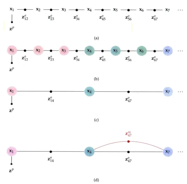
5-4 Factor graph model for dense reconstruction . . . . 116

5-5 Factor graph model for dense reconstruction (continued from figure 5-4) . . 117

5-6 Lossy Incremental Segmentation -sample results . . . . 118

5-7 Ship hull data set 2018-03-14.00.30-69: Odometry-based pose estimates. . 123 5-8 Lossy Incremental Segmentation -sample results . . . 124

5-9 Ship hull data set 2018-03-14.00: perspective view . . . 126

5-10 Ship hull data set 2018-03-14.00: profile view . . . 127

5-11 Ship hull data set 2018-03-14.00: plan view . . . 128

5-12 Ship hull data set 2018-03-14.00: segmented point cloud P . . . 129

5-13 Ship hull data set 2018-03-14.00 -seed graph S . . . 130

5-14 Ship hull data set 2018-03-14.00 -Pairwise matches between surfels. . . . . 130

5-15 Dense SLAM: incremental updates . . . 131

5-16 Ship hull data set 2018-03-14.00 (segment): map uncertainty . . . . 133

6-1 Sensor offset measurement model . . . . 139

6-2 Hierarchical landmark concept . . . . 140

6-3 Implicit point range measurement model . . . . 141

List of Tables

2.1 Standard deviation values for a typical navigation payload . . . . 36

3.1 DIDSON ship hull data set -mixture model parameters . . . . 67

5.1 Odometry-based map accuracy . . . 132

5.2 SLAM-based map accuracy (no loop closures) . . . . 132

5.3 Factor graph parameters and run time performance . . . . 135

List of Acronyms

AHRS Attitude and Heading Reference System AUC area under curve

AUV Autonomous Underwater Vehicle

AWGN additive white Gaussian noise

DIDSON Dual-frequency Identification Sonar DVL Doppler velocity log

EKF extended Kalman filter

GNSS Global Navigation Satellite System

HAUV Hovering Autonomous Underwater Vehicle ICM Iterative Conditional Modes

ICP Iterative Closest Point

IHO International Hydrographic Organization

IMU Inertial Measurement Unit

INS Inertial Navigation System

KLD Kullback-Leibler divergence

LBL Long Baseline

MAP maximum a-posteriori

MBES Multibeam Echo Sounder MRF Markov Random Field

NTP Network Time Protocol

PPS Pulse-per-second

PTP Precision Time Protocol

ROC Receiver Operating Characteristic

ROV Remotely Operated Vehicle

SA Simulated Annealing

SAS Synthetic Aperture Sonar

SLAM Simultaneous Localization and Mapping TVG time-varying gain

USBL Ultra-Short Baseline

Notation

Variables

x - scalar

x -vector (assumed column vector) X, or X -matrix X - set

Operators

Reference Frames

Fp _{- a point whose coordinates are expressed in the reference frame F}

Fx -_{a pose whose coordinates are expressed in the reference frame F}

wT

F

W(wp WTFP)

Whenever an orientation of a pose is expressed in terms of its yaw, pitch, and roll (p, 0, p), these follow the rotation sequence Z-Y-X.

Chapter 1

Introduction

1.1

Motivation

Hidden under the commonly referenced adage that "we know more about the surface of the

Moon than we do about the oceanfloor" lies what is still a great unknown. From shipwrecks to

mountains, many important features remain unresolved in most maps of the ocean floor. As of this writing, full bathymetric coverage of the ocean basins has only been achieved at a spatial resolution of 5 kilometers, using a combination of highly accurate satellite altimetry and gravimetric models. The General Bathymetric Chart of the Ocean's Seabed 2030 project, which plans to create high resolution maps of the world's oceans by the year 2030, aims for 93% coverage for depths greater than 200 meters at a spatial resolution of 100 meters. Using current methods, this task is expected to require 350 years of ship time at a cost in the order of billions of dollars [32]. This stands in stark contrast with most land maps: the TerraSAR/TanDEM-X satellite formation, for instance, uses synthetic aperture radar to achieve a vertical accuracy of 4 meters at a resolution of 12 meters, with revisit periods of less than two weeks. Civilian optical satellites achieve even more impressive results, with the Pleiades constellation attaining 0.5 meters spatial resolution. If ocean basins are to be mapped at a comparable resolution (10 meters), then the need for high-resolution, autonomous mapping technology is clear: with the ability to operate at depths of up to

6000 meters' for over a day, Autonomous Underwater Vehicles (AUVs) can cover large

swaths of terrain without the presence of a support ship other than for launch and recovery. Survey operations performed by an AUV fleet, and supported by a single ship, have been demonstrated successfully in the past few years, pointing in a very promising direction to obtain such high resolution maps.

1_{This is currently the highest depth rating on a commercial AUV system (Kongsberg's Hugin and Remus} 6000 AUVs), allowing access to more than 95% of the world's ocean basins.

Before proceeding further, however, we must first support our emphasis on the need for high resolution; after all, uses for very accurate, high resolution maps of abyssal plains, for instance, may not be immediately obvious. The International Hydrographic

Organiza-tion (IHO) Standards for Hydrographic Surveys, for instance, require a maximum horizontal uncertainty of 2 meters at a 95% confidence level for its most strict survey grade, but these are only required in certain shallow water areas [94]. Since the end-use of most of these sur-veys is the elaboration of nautical charts, this is deemed sufficient accuracy for navigation purposes. Still, there are many important applications where the accuracy and resolution needs are much stricter, of which we list a few examples below.

1.1.1 Environmental Monitoring Nuclear Waste Dump Sites

Between 1946 and 1993 the amount of radioactivity from radioactive waste dumped in the oceans reached a maximum of 4.5 x 104 TBq2; it has since decreased (through decay) to less than half of this value. The waste dumped at these sites ranges from low-level solid waste to full nuclear reactor vessels with spent fuel; the northeast Atlantic alone contains well over 100,000 tons of waste containers [40]. In addition, there are also radioisotope ther-moelectric generators, nuclear warheads, and reactors (in the wrecks of nuclear-powered military vessels) whose locations are not known precisely [39]. Locating and monitoring these sites requires the use of platforms that can withstand full ocean depth (6000 me-ters) and produce maps with sufficient resolution to resolve small scale features, such as corrosion on a nuclear warhead or waste container.

1.1.2 Explosive Ordinance Disposal (EOD)

Detection and removal of explosive devices such as limpet mines is an important task for navies worldwide. This is often accomplished through a combination of trained marine mammals, divers, and small remotely operated vehicles, all of which have considerable drawbacks. The deployment of divers and/or trained marine mammals exposes them to very hazardous environments and, with the latter, it is often hard to ensure complete hull coverage. Similarly, while small ROVs are agile, they have very limited navigation and manipulation capabilities, which hinders their ability to localize and neutralize a device.

Unexploded ordinance (UxO) disposal is not limited to active ships, as exemplified by the SS Richard Montgomery. This Liberty-class cargo ship was wrecked in the Thames Estuary during World War II while carrying munitions. The 1400 tons of explosive cargo

1.1. MOTIVATION

that remain in the wreck and its proximity to inhabited areas pose a significant hazard, which has led to the creation of an exclusion zone around the wreck, as well as periodic surveying to monitor its condition [97].

1.1.3 Inspection, Maintenance, and Repair (IMR)

One of the underwater mapping applications for which there is growing commercial de-mand is the inspection, maintenance, and repair of subsea infrastructure. These applica-tions comprise a variety of tasks, such as inspecting long pipelines that connect wells to manifolds, surveying "christmas trees", and operating equipment [5, 57]. At the present, most of these tasks are performed using Remotely Operated Vehicles (ROVs), which re-quire skilled pilots and the deployment of expensive support ships. This has sparked the development of inspection platforms that can perform some of these tasks autonomously, thereby reducing some of the major costs associated with IMR operations [16].

1.1.4 Search and Rescue (SAR)

The last ten years have witnessed a few high profile accidents where AUVs, ROVs, and other underwater mapping platforms have played a crucial role in the search and recovery efforts.

Air France flight 447

Air France flight 447 crashed into the Atlantic Ocean on June 1st, 2009, after the airplane entered a high-altitude stall condition from which it did not recover. Efforts to find the missing airplane and its black boxes began almost immediately, but proved unfruitful, with the third search phase ending in late May of the following year [102]. The debris field was finally identified during a fourth search phase in early April 2011, from side-scan sonar data obtained by REMUS 6000 AUVs operated by the Woods Hole Oceanographic Institution (WHOI). A second pass over the debris field provided photographic cover-age which was critical to the successful recovery of both the flight data and cockpit voice recorders by an ROV [28].

Malaysia Airlines flight 370

The circumstances behind the disappearance of Malaysia Airlines Flight 370 on March 8, 2014, remain unknown', despite the most costly search effort in history, involving a vari-ety of assets and equipment from nine different countries. This search was also notable

3

The description of the search for MH370 is based on the known facts as of the time of this writing.

for highlighting the lack of detailed maps in many areas of the ocean. Specifically, ar-eas for which the only available maps had a resolution of 5 kilometers per pixel, have now been mapped using high resolution multibeam echo sounders and synthetic aper-ture sonars, which can resolve feaaper-tures that are 100 times smaller [79]. In the process, four shipwrecks were found, as were topological features as large as underwater volca-noes [107, 125]. Given the configuration of the search area and the harsh sea conditions faced by the survey vessels, sonar-equipped towed bodies were the platform of choice for mapping operations. AUVs were a key component of the last search phase, in which the survey company Ocean Infinity deployed a fleet of eight Kongsberg Hugin AUV to cover in excess of 100,000 square kilometers. The same AUV fleet has also been deployed to find the wrecks of South Korean tanker Stellar Daisy and Argentinian submarine ARA San Juan.

Having motivated the need for high resolution mapping, we must now move on to the key factors behind it. The accuracy of a map depends mainly on the individual accuracies of:

(i) the estimate of the position and orientation (pose) of the mapping in some global frame,

(ii) the estimates of the offsets between the mapping sensors, the platform, and its navi-gation sensors, and

(iii) the mapping sensor measurements.

In the following sections, we provide some examples of the typical navigation and map-ping payloads used in underwater reconstruction applications.

1.2 Navigation Sensors

For underwater platforms, the rapid attenuation of electromagnetic (EM) signals in water precludes the use of Global Navigation Satellite System (GNSS) receivers at any meaning-ful depth. Underwater analogues to GNSS-acoustic positioning systems such as Long Baseline (LBL) and Ultra-Short Baseline (USBL) -can attain meter-level (or better) accu-racy in platform position estimates, but have significant drawbacks [77]. LBL requires the deployment of a minimum number of beacons, which need to be surveyed before they can be used for positioning. USBL, on the other hand, requires a surface-deployed transponder with a known position-often a GNSS-equipped support-ship. The attenuation of sound in water and its comparatively slow speed (with respect to EM waves) places limits on both the coverage and update rate offered by these systems. Finally, it is also important

1.3. MAPPING SENSORS

to note that when used in acoustically complex environments, these systems are subject to undesirable phenomena such as occultation, reverberation and multi-path propagation, which can significantly degrade their positioning performance.

Nearly all inspection and mapping platforms rely on some form of dead-reckoning as their primary source of pose estimates. This often takes the form of a Doppler veloc-ity log (DVL)-aided Inertial Navigation System (INS), in which the body-relative bottom velocity is first transformed to and integrated in the local-level frame (described in sec-tion 1.5) using an attitude estimate from an on-board Attitude and Heading Reference System (AHRS)4 [11, 47,48,49,27,121]. The performance of these systems, often described by the horizontal position uncertainty as a percentage of distance traveled, is mostly

de-termined by the accuracy of the velocity and yaw measurements. Noise in the velocity estimate will cause an unbounded growth (random walk) in the position estimate; this is made worse by the drift in the yaw estimate found in most INSs. One of the main limi-tations of dead-reckoning DVL-aided INSs is that bottom-relative velocity measurements are only available below a certain altitude (distance from the seafloor); above this, the DVL can provide velocity measurements relative to the water mass, which requires estimating water column velocity to obtain a global position estimate. This is often accomplished through the use of kinematic and dynamic vehicle models [33].

1.3 Mapping Sensors

Most of the sensors used in underwater mapping platforms fall in one of two categories:

acoustical and optical. While the former have long been the backbone of most, if not all,

mapping efforts, recent advances in underwater optical systems have enabled the deploy-ment of inspection platforms with metrology-grade lidar systems.

1.3.1 Optical Mapping Sensors

Optical mapping sensors include camera-based, structured light, and lidar systems. These sensors offer very high resolution (1-10 millimeters), but often at the expense of power or range: between the lighting systems required by cameras and the high-intensity lasers used in both structured light and lidar sensors, it is not uncommon for optical systems to require power in the range of 50 to 150 watt. At the same time, the range of these sensors is limited by the water conditions: while clear water environments can allow for ranges

4

Like an INS, an AHRS has an inertial measurement unit at its core; the difference between the two being that an AHRS is used exclusively for orientation estimates, whereas an INS is used for both position and orientation estimates. More advanced INS may also estimate body velocity, local gravity vector and other parameters.

in excess of 40 meters for high-power lidars, turbid environments such as harbors and coastal areas can see the maximum range of such sensors decrease to a few meters. As both structured light and lidar sensor are prohibitively expensive for all but high-end inspection mapping platform, camera-based systems are the most common of the three, with stereo cameras proving a very cost-effective option for high-resolution optical mapping.

1.3.2 Acoustic Mapping Sensors

Acoustic mapping sensors have evolved from simple pencil-beam echo sounders to a wide variety of sensors, including three-dimensional imaging systems and Synthetic Aperture Sonars (SASs). The most commonly used sonars for mapping, however, are side-scan sonars and Multibeam Echo Sounders (MBESs). The former can often be found in towed bodies and torpedo-shaped AUVs, as their wide swath combined with the platform ve-locity produces high coverage rates. Because of their inability to capture terrain geometry, they are often complemented by profiling5 multibeam sonars. As with all sonars, the at-tenuation of sound forces multibeams to operate on a trade-off between resolution and range: low-frequency sonars can reach distances beyond 10 kilometers at low resolution; high frequency models attain centimeter resolution but are often limited to distances of up to a few tens of meters. One of the main advantages of high-frequency multibeam sonars, despite their limited range, is their robustness to turbidity, which allows them to operate in high turbidity environments, such as the ones mentioned above. Advances in sensor technology, and the combination of Moore's law and Dennard scaling6 have enabled the appearance of the first real-time three-dimensional sonars [17, 64].

As most of the research in this dissertation was motivated by the problem of ship hull inspection, it is safe to assume that the water conditions encountered by an inspection platform will often be turbid-this has certainly been the case in all the data collection deployments for which results are presented. The short visual range (usually in the range of 1-2 meters, but falling below 1 meter in certain conditions), combined with the need to operate safely when inspecting geometrically complex areas, such as the running gear of a large ship, motivates the use of sonar for a major part of the mapping and inspection

5

A profiling multibeam has a narrow vertical field of view, and is pointed perpendicularly to the terrain,

producing a scan that is similar to a "slice" of the scene along the scanning plane. An imaging multibeam has a wider vertical field of view (tens of degrees), and is pointed at an angle, yielding scans that are similar to those of a camera.

6

While Moore's law describes the doubling in the number of transistors (in an integrated circuit) every two years brought about by miniaturization, Dennard scaling states that their power density remains constant -the combination of -the two implies that performance per watt doubles every two years. This allows for -the computational resources in both sensors and platforms to grow at the same rate while keeping the same power budget.

1.4. RELATEDWORK

tasks. For this reason, we will focus on the high-frequency profiling multibeam sonar as the primary mapping sensor. This does not preclude the use of other sensors; in fact, the techniques described in the following chapters can easily be extended to work using data from structured light or lidar sensors.

1.4 Related Work

Most of the work in high-resolution underwater mapping can be split into one of two

cat-egories: featureless and feature-based approaches, depending on their use of environmental

features to describe the scene. The ubiquity of multibeam echo sounders, in combination with the ambiguities in both camera and side-scan features (as well as the limited compu-tational resources available to identify, track, and match such features) meant that early work on underwater mapping was often accomplished using featureless approaches. As both sensor and computer technology develop, however, feature-based techniques are be-coming ever more popular and successful.

1.4.1 Feature-based techniques

Feature-based techniques are commonly found in methods using imaging-type modalities, such as cameras, imaging, and side-scan sonars [23, 24, 41, 80, 81]. The main challenges

faced by these approaches are the feature sensitivity to the ensonification (sonar) or light-ing (camera) conditions, as well as the ambiguity associated with the location of the feature with respect to the sensor, as both cameras and imaging sonar provide under-constrained measurements.

1.4.2 Featureless techniques

When the primary mapping sensor provides data that is closer to a range measurement, the use of featureless techniques is more prevalent. This is the case with profiling multibeam echo sounders, as well as other sonars where the narrow beam widths allow for small azimuth/elevation ambiguities in range measurements.

Much of the early research on simultaneous localization and mapping in underwater environments has addressed the problem from a two-dimensional perspective, where the platform pose comprises its position and orientation in the horizontal plane. Many of these techniques employ single-beam, mechanically-scanned imaging sonars, whose 360 coverage makes them well-suited to some of the scan-matching techniques that have been proven successful in land applications [54]. Unlike the lidars used by their terrestrial coun-terparts, the scanning sonars used by these underwater robots have cycle times that are

comparable to, and often slower than, the vehicle dynamics. To avoid the motion-induced artifacts that result from this limitation, some of the techniques will either assume-or keep-the vehicle in-place while a full scan is assembled [61]. Platforms equipped with dead-reckoning sensors relax this operational limitation by relying on the pose estimate that these sensors provide to compensate for vehicle motion while the scan is assembled

[58,59].

Extending featureless techniques to three dimensions shares some of the challenges with the previously described planar mapping techniques: just as these have to address the constraints imposed by the scanning sonar, the same holds for many three dimensional mapping methods. This limitation, as described earlier in this chapter, stems from the op-erational constraints imposed by profiling multibeam sonars, as attaining reasonable cov-erage rates requires moving perpendicularly to the scanning plane, which removes any overlap between scans, hence precluding the direct use of scan-matching techniques. To circumvent this limitation, the standard approach is to assemble maps over small spa-tial scales using a limited number of scans. These submaps, similar to virtual 3D sonar measurements, can then be pairwise registered. Such techniques have been successfully demonstrated in microbathymetric applications [83, 84, 82, 85], where the 2.5D nature of the scene (elevation model) allows the submaps to be treated as images and leverage image registration methods.

Some sensor and platform configurations can avoid the need to create submaps: the volumetric range measurements produced by 3D sonars allow for direct pairwise regis-tration of scans [65]. The DEPTHX robot, for instance, was equipped with 54 pencil-beam sonars arranged in three perpendicular rings, allowing for partial position measurements with respect to a current map estimate to be obtained. Using occupancy grids as its map representation, this platform was used to produce maps of flooded sinkholes with a reso-lution of a few tens of centimeters [26]-this representation, well-suited for use with sonar, had also been used two decades earlier in some of the first ship- and ROV-based mapping efforts [100]. DEPTHX's highly-accurate gyro-compass and depth sensor pair allowed the orientation and depth measurements to be considered as drift-free estimates, thereby sim-plifying the full pose estimation problem to that of estimating the platform's horizontal position, which was accomplished using a particle filter.

1.4.3 Hybrid approaches

It is also worth noting that there exist hybrid approaches, combining both feature-rich camera data with the ranging measurements obtained from multibeam sonar [50, 51, 70, 71, 73, 74, 72, 75]. In one of the earliest approaches combining the two modalities, a sonar is used to obtain the terrain profile and initialize the extraction of visual features [56, 122].

1.5. REFERENCE FRAMES

These features are added to an extended Kalman filter (EKF) Simultaneous Localization and Mapping (SLAM) framework, and tracked between successive frames. The use of sonar information reduces the ambiguity in the visual features, and allows for the estima-tion of elevaestima-tion and azimuth measurements for each tracked feature. These methods are demonstrated experimentally by the mapping of sections of coral reef.

1.5 Reference Frames

The main reference frames used in this work are [27, 68]:

" World frame (W) - this is the global, Earth-fixed frame, which follows the NED (North-East-Down) convention for the orientation of its axes.

" Local-level frame (L) - also known as the tangent, or vehicle-carried frame, this frame has its axes parallel to the world frame, but its origin is coincident with that of the platform frame.

" Platform frame (P) - the platform or body-fixed frame is located at some reference point in the platform, and its axes follow the Forward-Port-Down convention.

" Navigation frame (N) - this is the reference frame used by the navigation package, whose estimate describes the transformation from the world to this frame. Through-out the text we assume that the offset between the navigation and platform frames are known and accounted for, so that the pose estimates describe the pose of the

platform frame in the world frame.

" Sensor frame (S) -similarly to the navigation frame, this is the reference frame used

by the mapping sensor. Depending on the platform configuration, several of these

frames may exist (e.g. camera, multibeam, lidar).

1.6 Assumptions

The main assumptions made in the course of this work are:

- A pose estimate is availablefrom the platform -as mentioned in section 1.2 most, if not all mapping platforms, carry some form of aided inertial navigation system whose short-term accuracy is is sufficiently high to obtain small scale maps; the consequence of this assumption is that we can build upon these estimates to focus on the recon-struction problem and on how to address the medium- and long-term drift that these

systems exhibit. Moreover, by not requiring a specific navigation architecture, the so-lutions proposed in chapters 4 and 5 can also be extended to incorporate individual navigation sensor measurements. Finally, it is worth noting that this assumption is commonly made in the underwater mapping literature [24].

- The travel time of the sonar signal can be considered instantaneous -In order to produce high resolution maps, mapping platforms will employ high-frequency (>1 mega-hertz) multibeam echo sounders. Due to the high attenuation at these frequencies, the effective range of these sonars is often under 10 meters, which corresponds to a two-way travel time of less than 3 milliseconds. Given the typical mapping platform moves at speeds of less than 2 meters per second, the effects of the finite travel time

are assumed negligible.

- Sound refraction can be neglected -the relatively small volume ensonified by the multi-beam echo sounder is considered well-mixed and sufficiently uniform so that the effects of refraction due to water density variations are negligible.

- All sensors are synchronized -a modern underwater mapping platform will often con-tain a network of computers: most sensors will carry their own embedded system and communicate with the main computer, where data is stored, processed and/or relayed, via some combination of serial or network protocol. While most of these sys-tems will not be equipped with accurate clocks, many solutions exist to keep them in relative synchrony. Both the Network Time Protocol (NTP) and the Precision Time Protocol (PTP), as well as on-board Pulse-per-second (PPS) signal distribution and triggering schemes can be used to keep timing differences between systems to within milli- or even micro-seconds.

- Sensor offsets have been calibrated prior to platform deployment - chapter 2 describes the three dominant factors in reconstruction accuracy; while sensor offsets are one of them, they are often estimated to a sufficient degree of accuracy during pre-mission operations and considered fixed for the remainder of the mission.

- The accuracy limitations of a local Cartesian coordinate frame are negligible -we assume that the scene is small enough that the limitations of a local Cartesian frame can be considered negligible with respect to other sources of uncertainty.

Chapters 3 through 5 will describe the motivations for these assumptions and, where nec-essary, introduce other minor assumptions. Section 6.2.1 will revisit the main assumptions and provide remarks on how some of these can be relaxed.

1.7. CONTRIBUTIONS

1.7 Contributions

The contributions presented in this dissertation aim at improving the accuracy of maps of underwater scenes produced from multibeam sonar data. The main contributions are summarized below:

- _{First, we propose robust methods to process and segment sonar data to obtain} accu-rate range measurements in the presence of noise, sensor artifacts, and outliers [105]. These methods attempt to model acoustic phenomena such as attenuation and beam pattern to recover an improved estimate of the sonar data that is then fed to either a dense or sparse _{segmentation technique. In the dense approach, a label is computed} for every range-azimuth cell in the scan from an intensity distribution model esti-mated online; in the sparse approach, a label is estiesti-mated for every beam.

- _{Second, we propose a volumetric, submap-based SLAM technique that can} success-fully leverage map information to correct for drift in the mapping platform's pose es-timate [104]. Submaps are small, self-consistent maps obtained by grouping together scans over short periods of time, which enable the use of scan-matching techniques to derive loop closures. The reduction in the number of poses brought about by the use of submaps also allows the proposed technique to be used in real-time applica-tions.

- _{Third, and informed by the previous two contributions, we propose a dense} ap-proach to the sonar-based reconstruction problem, in which the pose estimation, sonar segmentation and model optimization problems are tackled simultaneously under the unified framework of factor graphs [106]. This stands in contrast with the traditional approach where the sensor processing and segmentation, pose estima-tion, and model reconstruction problems are solved independently.

For each of the techniques described above, we provide experimental results that validate the proposed methods. These were obtained over several deployments of a commercial inspection platform, under the scope of the Office of Naval Research's ship hull inspection project.

1.8 Overview

This dissertation is structured as follows: Chapter 2 motivates and describes the overarch-ing mappoverarch-ing and pose estimation problems in a more formal fashion. Chapter 3 addresses the processing and segmentation of data from the primary mapping sensor-the multi-beam echo sounder-to obtain measurements that can be used to create a model; chapter 29

4 builds upon these results and describes a submap-based technique that can be used to produce maps in real time while simultaneously mitigating the effects of the drift in the position estimates from the on-board navigation system. Chapter 5 aims at bringing the two problems together under a unified framework to not only address some of the key lim-itations of the technique presented in chapter 4, but also to leverage the problem of model optimization to improve the accuracy in both the sensor range and pose estimates. Finally, chapter 6 offers some concluding remarks on the proposed techniques, revisits some of the key assumptions made in the process, and describes promising directions for future work.

Chapter 2

Problem Statement

2.1

Introduction

This chapter describes the problem of high resolution mapping, to arrive at a model for the mapping error/uncertainty as a function of its three main components: pose estimate uncertainty, sensor offset uncertainty, and sensor measurement uncertainty.

2.2

Problem Formulation

The problem of producing an accurate map of a scene can be stated as one where we wish to spatially register sensor data in the world frame. Depending on the intended use of the map, it may have to fulfill certain requirements -navigation charts, for instance, must comply to the IHO's Special Publication 44 [94]. This standard specifies minimum accuracy requirements for different survey classes, which are expressed in terms of the maximum allowable values (2o-) for the horizontal and vertical uncertainties in the positioning of soundings, measurements, aids to navigation, and other relevant features.

Assuming the primary mapping sensor measures the position of some feature or object point in its own frame Sx, _{that position can be registered in the world frame by}

"'x =VT

PT

where "T is the platform's pose in the world reference frame, and PT is the sensor pose in the platform frame. As previously mentioned, map accuracy is a function of the un-certainty associated with the position of this feature or point in the world frame which, in turn, depends on the uncertainty associated with each of the terms on the right hand side of equation (2.1).

In practical applications there are often more reference frames at play, with at least one for each sensor used in navigation (e.g. DVL, Inertial Measurement Unit (IMU), pressure sensor, ... ) or mapping (e.g. cameras, lidar, multibeam sonar, ...). As some of these will be mounted on actuators, such as a pan/tilt mount, the pose of some of these frames with respect to the platform may vary over time. Since these frames are tied to the actual configuration of the mapping platform, we will instead consider a more general model using just the following three reference frames: world, platform, and sensor. In the next section we will propose simple models for how the uncertainty in the estimates associated with these frames impacts mapping performance over time.

2.2.1 Sensor Performance

In equation (2.1), we assumed the mapping sensor provided the position of an object point or feature in its own frame, Sx. In fact, it is often the case that these sensors instead provide a range measurement to that point or feature, T, along a nominal measurement direction

b. While this "single measurement" sensor model may appear overly simplistic, it can easily be extended to describe more typical sensors outputting a set of such measurements,

(Ti, bi), such as sonars or lidars.

Assuming an unbiased sensor, we can model the range measurement as

i, = r,

+ vr

where the measurement noise Vr will follow some probability distribution which, for the sake of this discussion, we will approximate as a zero-mean normal distribution with stan-dard deviation or . This range measurement is projected along the sensor's nominal point-ing direction b to register the measurement in the sensor's reference frame:

sx=

b,.

Depending on the nature of the sensor, there will be a varying degree of uncertainty on the direction b, which may be captured by the degree of accuracy in the sensor's calibration, or by some other sensor property such as the beam pattern for acoustic or electromag-netic transducers such as sonar or radar. Parameterizing the unit vector's orientation with azimuth and elevation angles a and 0, again subject to some normally-distributed noise

1

As expected, range measurement noise is likely to follow some other distribution that is significantly different from the normal distribution, and likely multimodal. One such example can be found in acoustics-based range measurements, where phenomena such as refraction and multi-path can significantly skew range measurements while also introducing multiple modes in the range distribution.

2.2. PROBLEM FORMULATION

around their nominal values

S+V(2.4)

we can express the nominal pointing direction as

cos cos a

cos sin& . (2.5)

Lsin

J

Under these assumptions, the position of the range measurement in the sensor frame will follow a normal distribution centered around the true position, s sx = br, and with

covariance s = , where

J

Jacobian

(2.3) [96]

cosacosp -rsina cos§ -rcosasinp

J= sintacosp r cos a cos

P

sin

p

Note that this is an approximation for the true distribution associated with 'x,, and is only valid for small values of oc-, p; if large deviations from the nominal measurement

direction are expected, the resulting distribution cannot be reasonably approximated by a multivariate normal in Cartesian space.

2.2.2 Sensor Offsets

The position of the range measurement in the platform frame is

Xp = Pxs + Rsxp (2.7)

where Pxs and PR are the sensor position and orientation in the platform frame, with as-sociated uncertainties PEP = diag([ cr, 2 ]) andE = diag([o

o

using a yaw (p), pitch (0), roll (q) - YPR - attitude parameterization. Under the small an-gle assumption, the uncertainty in the position of the range measurement in the platform frame can be approximated by a normal distribution with mean Px, and covariance

E= +A ) + R PE,) RT (2.8)

where

JA

(2.7) comprising the partial derivatives with respect to orientation (again, under a YPR

parameterization). For the special case where the estimate of the offset between platform

and sensor frames is sufficiently accurate that small angle perturbations can be considered (1p, 0, p 0 ==-> sR ~ 13x3),

lB

IA = sx 0 _sz, (2.9)

. 0 _sXP s Y

The three terms on the right side of equation (2.8) correspond to the contributions due to uncertainty in sensor translation, orientation, and range measurement (respectively). The alignment assumption above makes it easier to see that, for large range measurements, un-certainty in sensor orientation, rather than position, is the dominant factor in registration accuracy.

2.2.3 Navigation Performance

To model the remaining component of the right-hand side of equation (2.1), we introduce a simple dead-reckoning model, based on a rate-integrating gyroscope and body-relative velocity measurements. This is a planar analogue to the DVL-aided inertial navigation systems found in many underwater platforms [48].

In this model, vehicle kinematics are limited to the horizontal plane and approximated by a simple integrator, where the state vector x - [x y p]T represents position (x,y) and

heading p. The control input u = [u v wz]T corresponds to the linear velocity in the horizontal plane (u, v), and angular velocity component along the platform's z axis, wz. The vector v, known as the process noise, accounts for uncertainty in the model, and is assumed to be zero-mean and normally distributed, with covariance E.

x=u-

+

Under this simple model, the uncertainty associated with the state estimate, P, will grow over time, as described by

1 =(2.11)

To produce a pose estimate, we drive the model described by equation (2.10) with an esti-mate of u. While this estiesti-mate can be derived from commanded values (set points), most estimators will instead rely on measurements

a.

X = U (2.12)

2.2. PROBLEM FORMULATION

estimate i to diverge from the true state x - this is captured by the increase in the uncer-tainty associated with the state estimate, P. This growth is governed by models of the measurements used to drive the model, as explained below.

Angular speed measurement model

In the absence of an absolute heading reference, a heading estimate i can be computed

by integrating angular velocity measurements coming from a gyroscope. These

measure-ments are typically contaminated with additive white Gaussian noise (AWGN), v,,, and a non-zero (uncompensated) bias, modeled as a random walk driven by process noise b,

(also AWGN).

&)z = wz + bz Wz=Wz~z+Vwz(2.13)

+

Linear velocity measurement model

Velocity sensors measure the platform velocity with respect to an external reference, such as the local terrain or the surrounding water column. These measurements are also as-sumed to be contaminated with AWGN v.

bUb =b Ub + Vu (2.14)

Using the heading estimate

4,

estimate [i §]T. Augmenting the system model (equation 2.12) with the measurement models used to drive it (equations 2.13 and 2.14), the estimate will evolve according to

0

£

cos(*)

0

19

sin(p)

1

i

O IbJ.

0

0

oV

x = Ai+ B(x)u+C(x)v

and the associated covariance

P=

[j

I'

-o1

Parameter Measurement/Parameter Axis Value Units Reference

eu

0V body-relative velocity by 0.001 m.s 1 [1241

oW angular velocity bz 0.1 rad.s- [34] Ojbz angular velocity bias bz 0.3-3 mrad.s1 [34]

"z depth WZ 0.25 m [35]

Table 2.1: Standard deviation values for a typical navigation payload comprising a Doppler velocity log (DVL), an AHRS or tactical-grade IMU, and a pressure sensor. The standard deviation in the depth measurement assumes an accuracy of 0.25% of full scale (assumed to be 100m).

Note that the need to project the body velocity in the world frame (using the heading estimate ^) makes the model non-linear.

2.2.4 Map Accuracy

The position of the sonar measurement in the world frame is Wx

= xp

+

+

where Wxp and WR are the position and orientation of the platform in the world frame. The uncertainty associated with this range measurement, expressed in the world frame, can be obtained using the same approach as in subsection 2.2.2, yielding

W = Et + IA

(WEa)

where the WEt and WE, terms are the uncertainty in the position and attitude of the plat-form (respectively). The covariances for the noise models driving this equation are listed in table 2.1. The term PE,, capturing the uncertainty in the measurement in the platform frame, is defined by equation 2.8.

The discussion above describes a "decoupled" navigation filter, where estimates for the horizontal and vertical position components are obtained independently. This approach, while simple, provides a good approximation to the navigation schemes found in the lit-erature and used by several underwater platforms [48, 49].

Chapter 3

Multibeam Data Processing

3.1 Introduction

The purpose of this chapter is to introduce the primary mapping sensor-the multibeam sonar-and the techniques used to process its data so as to derive measurements that can be spatially registered using the chosen map representation. To do this, we begin with an overview of the operating principles behind the sonar and how these are used to produce an image. We then state the segmentation problem, which must be solved in order to ob-tain a set of range measurements that can be spatially registered. Before moving on to the problem of segmentation, however, we discuss some important pre-processing techniques that can be used to mitigate noise and other artifacts present in these images that will oth-erwise affect the accuracy of the range estimates. We address the segmentation problem with two alternative approaches: the first estimates target and background intensity dis-tributions to obtain a per-pixel (dense) segmentation; the other assumes a signal with a known envelope may exist in the received reflection and estimates its location to obtain a range estimate directly. Both techniques are extended to take advantage of underlying scene geometry. Finally, we demonstrate and compare the proposed approaches with the standard fixed-threshold segmentation technique using experimental data.

While the main focus of this chapter is on the processing and segmentation of multi-beam profiling sonar data, the proposed approaches generalize well to other single- or multi-beam sensors which measure received reflection intensity as a function of time or range, with radar based systems being a prime example.

37