HAL Id: hal-02611689
https://hal.archives-ouvertes.fr/hal-02611689
Submitted on 2 Jun 2020
HAL is a multi-disciplinary open access
archive for the deposit and dissemination of
sci-entific research documents, whether they are
pub-lished or not. The documents may come from
teaching and research institutions in France or
abroad, or from public or private research centers.
L’archive ouverte pluridisciplinaire HAL, est
destinée au dépôt et à la diffusion de documents
scientifiques de niveau recherche, publiés ou non,
émanant des établissements d’enseignement et de
recherche français ou étrangers, des laboratoires
publics ou privés.
model simulations under uniform changes in CO2
temperature, water, and nitrogen levels (protocol
version 1.0)
James Franke, Christoph Müller, Joshua Elliott, Alex Ruane, Jonas
Jägermeyr, Juraj Balkovic, Philippe Ciais, Marie Dury, Pete Falloon,
Christian Folberth, et al.
To cite this version:
James Franke, Christoph Müller, Joshua Elliott, Alex Ruane, Jonas Jägermeyr, et al.. The GGCMI
Phase 2 experiment: global gridded crop model simulations under uniform changes in CO2
temper-ature, water, and nitrogen levels (protocol version 1.0). Geoscientific Model Development, European
Geosciences Union, 2020, 13 (5), pp.2315-2336. �10.5194/gmd-13-2315-2020�. �hal-02611689�
https://doi.org/10.5194/gmd-13-2315-2020 © Author(s) 2020. This work is distributed under the Creative Commons Attribution 4.0 License.
The GGCMI Phase 2 experiment: global gridded crop model
simulations under uniform changes in CO
2
, temperature,
water, and nitrogen levels (protocol version 1.0)
James A. Franke1,2, Christoph Müller3, Joshua Elliott2,4, Alex C. Ruane5, Jonas Jägermeyr2,3,4,5, Juraj Balkovic6,7, Philippe Ciais8,9, Marie Dury10, Pete D. Falloon11, Christian Folberth6, Louis François10, Tobias Hank12,
Munir Hoffmann13,22, R. Cesar Izaurralde14,15, Ingrid Jacquemin10, Curtis Jones14, Nikolay Khabarov6, Marian Koch13, Michelle Li2,16, Wenfeng Liu8,17, Stefan Olin18, Meridel Phillips5,19, Thomas A. M. Pugh20,21, Ashwan Reddy14, Xuhui Wang8,9, Karina Williams11,23, Florian Zabel12, and Elisabeth J. Moyer1,2
1Department of the Geophysical Sciences, University of Chicago, Chicago, IL, USA
2Center for Robust Decision-making on Climate and Energy Policy (RDCEP), University of Chicago, Chicago, IL, USA 3Potsdam Institute for Climate Impact Research, Member of the Leibniz Association, Potsdam, Germany
4Department of Computer Science, University of Chicago, Chicago, IL, USA 5NASA Goddard Institute for Space Studies, New York, NY, USA
6Ecosystem Services and Management Program, International Institute for Applied Systems Analysis, Laxenburg, Austria 7Department of Soil Science, Faculty of Natural Sciences, Comenius University in Bratislava, Bratislava, Slovak Republic 8Laboratoire des Sciences du Climat et de l’Environnement, CEA-CNRS-UVSQ, Gif-sur-Yvette, France
9Sino-French Institute of Earth System Sciences, College of Urban and Env. Sciences, Peking University, Beijing, China 10Unité de Modélisation du Climat et des Cycles Biogéochimiques, UR SPHERES,
Institut d’Astrophysique et de Géophysique, University of Liège, Liège, Belgium
11Met Office Hadley Centre, Exeter, UK
12Department of Geography, Ludwig-Maximilians-Universität München, Munich, Germany
13Georg-August-University Göttingen, Tropical Plant Production and Agricultural Systems Modeling, Göttingen, Germany 14Department of Geographical Sciences, University of Maryland, College Park, MD, USA
15Texas Agrilife Research and Extension, Texas A&M University, Temple, TX, USA 16Department of Statistics, University of Chicago, Chicago, IL, USA
17EAWAG, Swiss Federal Institute of Aquatic Science and Technology, Dübendorf, Switzerland 18Department of Physical Geography and Ecosystem Science, Lund University, Lund, Sweden 19Earth Institute Center for Climate Systems Research, Columbia University, New York, NY, USA 20School of Geography, Earth and Environmental Sciences, University of Birmingham, Birmingham, UK 21Birmingham Institute of Forest Research, University of Birmingham, Birmingham, UK
22Leibniz Centre for Agricultural Landscape Research (ZALF), Müncheberg, Germany
23Global Systems Institute, University of Exeter, Laver Building, North Park Road, Exeter, EX4 4QE, UK
Correspondence: Christoph Müller ([email protected]) Received: 23 August 2019 – Discussion started: 25 October 2019
Abstract. Concerns about food security under climate change motivate efforts to better understand future changes in crop yields. Process-based crop models, which represent plant physiological and soil processes, are necessary tools for this purpose since they allow representing future climate and management conditions not sampled in the historical record and new locations to which cultivation may shift. However, process-based crop models differ in many critical details, and their responses to different interacting factors remain only poorly understood. The Global Gridded Crop Model Inter-comparison (GGCMI) Phase 2 experiment, an activity of the Agricultural Model Intercomparison and Improvement Project (AgMIP), is designed to provide a systematic param-eter sweep focused on climate change factors and their in-teraction with overall soil fertility, to allow both evaluating model behavior and emulating model responses in impact as-sessment tools. In this paper we describe the GGCMI Phase 2 experimental protocol and its simulation data archive. A total of 12 crop models simulate five crops with systematic uni-form perturbations of historical climate, varying CO2,
tem-perature, water supply, and applied nitrogen (“CTWN”) for rainfed and irrigated agriculture, and a second set of simula-tions represents a type of adaptation by allowing the adjust-ment of growing season length. We present some crop yield results to illustrate general characteristics of the simulations and potential uses of the GGCMI Phase 2 archive. For ex-ample, in cases without adaptation, modeled yields show ro-bust decreases to warmer temperatures in almost all regions, with a nonlinear dependence that means yields in warmer baseline locations have greater temperature sensitivity. Inter-model uncertainty is qualitatively similar across all the four input dimensions but is largest in high-latitude regions where crops may be grown in the future.
1 Introduction
Understanding crop yield response to a changing climate is critically important, especially as the global food produc-tion system will face pressure from increased demand over the next century (Foley et al., 2005; Bodirsky et al., 2015). Climate-related reductions in supply could therefore have severe socioeconomic consequences (e.g., Stevanovi´c et al., 2016; Wiebe et al., 2015). Multiple studies using different crop or climate models concur in projecting sharp yield re-ductions on currently cultivated cropland under business-as-usual climate scenarios, although their yield projections show considerable spread (e.g., Rosenzweig et al., 2014; Schauberger et al., 2017; Porter et al., 2014, and references therein). Although forecasts of future yields reductions can be made with simple statistical models based on regressions in historical weather data, process-based models, which sim-ulate the effect of temperature, water and nutrient availabil-ity, and atmospheric CO2 concentration on the process of
photosynthesis and the biology and phenology of individual crops, play a critical role in assessing the impacts of climate change.
Process-based models are necessary for understanding crop yields in novel conditions not included in historical data, including higher CO2 levels, out-of-sample
combina-tions of rainfall and temperature, cultivation in areas where crops are not currently grown, and differing management practices (e.g., Pugh et al., 2016; Roberts et al., 2017; Mi-noli et al., 2019). Process-based models have therefore been widely used in studies on future food security (Wheeler and Von Braun, 2013; Elliott et al., 2014a; Frieler et al., 2017), options for climate mitigation (Müller et al., 2015) and adap-tation (Challinor et al., 2018), and future sustainable devel-opment (Humpenöder et al., 2018; Jägermeyr et al., 2017). They are a necessity for global gridded simulations, which al-low understanding the global dynamics of agricultural trade, because global market mechanisms can strongly modulate the economic impacts of regional yield changes (Stevanovi´c et al., 2016; Hasegawa et al., 2018). Global simulations are especially necessary in studying agricultural effects of cli-mate change (Müller et al., 2017), since systematic clicli-mate assessments must account for cultivation area changes and crop selection switching (Rosenzweig et al., 2018; Ruane et al., 2018) and must consider inter-regional differences (e.g., Nelson et al., 2014; Wiebe et al., 2015).
Modeling crop responses, however, continues to be chal-lenging, as crop growth is a function of complex interac-tions between climate inputs, soil, and management prac-tices (Boote et al., 2013; Rötter et al., 2011). Models tend to agree broadly in major response patterns, including a reason-able representation of the spatial pattern in historical yields of major crops and projections of shifts in yield under fu-ture climate scenarios (e.g., Elliott et al., 2015; Müller et al., 2017). But process-based models still struggle with some im-portant details, including reproducing historical year-to-year variability in many regions (e.g., Müller et al., 2017; Jäger-meyr and Frieler, 2018), reproducing historical yields when driven by reanalysis weather (e.g., Glotter et al., 2014), and low sensitivity to extreme events (e.g., Glotter et al., 2015; Schewe et al., 2019). Global models pose additional chal-lenges due to variable input data quality and limited ability for model calibration. Long-term projections therefore retain considerable uncertainty (Wolf and Oijen, 2002; Jagtap and Jones, 2002; Iizumi et al., 2010; Angulo et al., 2013; Asseng et al., 2013, 2015).
Model intercomparison projects such as the Agricultural Model Intercomparison and Improvement Project (AgMIP; Rosenzweig et al., 2013) are crucial in quantifying uncer-tainties in model projections (Rosenzweig et al., 2014). In-tercomparison projects have also been used to develop proto-cols for evaluating overall model performance (Elliott et al., 2015; Müller et al., 2017) and to assess the representation of individual physical mechanisms such as water stress and CO2fertilization (e.g., Schauberger et al., 2017). However, to
date, few such projects have systematically sampled critical factors that may interact strongly in affecting crop yields. A number of modeling exercises in the last 5 years have begun to use systematic parameter sweeps in crop model evalua-tion and emulaevalua-tion (e.g., Ruane et al., 2014; Makowski et al., 2015; Pirttioja et al., 2015; Fronzek et al., 2018; Snyder et al., 2019; Ruiz-Ramos et al., 2018), but all involve limited sites and most also limited crops and scenarios.
The Global Gridded Crop Model Intercomparison (GGCMI) Phase 2 experiment is the first global gridded crop model intercomparison involving a systematic parame-ter sweep across critical inparame-teracting factors. GGCMI Phase 2 is an activity of AgMIP, and a continuation of a multi-model comparison exercise begun in 2014. The initial GGCMI Phase 1 (Elliott et al., 2015; Müller et al., 2017) compared harmonized yield simulations over the historical period, with primary goals of model evaluation and understanding sources of uncertainty (including model parameterization, weather inputs, and cultivation areas); see also Folberth et al. (2019) and Porwollik et al. (2017) for more information. GGCMI Phase 2 compares simulations across a set of inputs with uni-form perturbations to historical climatology, including CO2,
temperature, precipitation, and applied nitrogen, as well as adaptation to shifting growing seasons (collectively referred to as “CTWN-A”). The CTWN-A experiment is inspired by AgMIP’s Coordinated Climate-Crop Modeling Project (C3MP; see Ruane et al., 2014; McDermid et al., 2015) and contributes to the AgMIP Coordinated Global and Regional Assessments (CGRA; see Ruane et al., 2018; Rosenzweig et al., 2018).
In this paper, we describe the GGCMI Phase 2 model ex-periments and present initial summary results. In the sections that follow, we describe the experimental goals and proto-cols; the different process-based models included in the in-tercomparison; the levels of participation by the individual models. We then provide an assessment of model fidelity based on observed yields at the country level, and show some selected examples of the simulation output dataset to illus-trate model responses across the input dimensions.
2 Simulation objectives and protocol 2.1 Goals
The guiding scientific rationale of GGCMI Phase 2 is to pro-vide a comprehensive, systematic evaluation of the response of process-based crop models to critical interacting factors, including CO2, temperature, water, and applied nitrogen
un-der two contrasting assumptions on growing season adapta-tion (CTWN-A). The dataset is designed to allow researchers to
– enhance understanding of models sensitivity to climate and nitrogen drivers;
– study the interactions between climate variables and ni-trogen inputs in driving modeled yield impacts; – characterize differences in crop responses to climate
change across the Earth’s climate regions;
– provide a dataset that allows statistical emulation of crop model responses for downstream modelers; and – explore the potential effects on future yield changes of
adaptations in growing season length. 2.2 Modeling protocol
The GGCMI Phase 1 intercomparison was a relatively lim-ited computational exercise, requiring yield simulations for 19 crops across a total of 310 model years of historical sce-narios, and had the participation of 14 modeling groups. The GGCMI Phase 2 protocol is substantially larger, involving over 1400 individual 30-year global scenarios, or over 42 000 model years; 12 modeling groups nevertheless participated. To reduce the computational load, the GGCMI Phase 2 pro-tocol reduces the number crops to five (maize, rice, soybean, spring wheat, and winter wheat). The reduced set of crops includes the three major global cereals and the major legume and accounts for over 50 % of human calories in 2016: nearly 3.5 billion tons or 32 % of total global crop production by weight (FAO, 2018). This set of major crops has the advan-tage of historical yield data globally available at subnational scale (Ray et al., 2012; Iizumi et al., 2014), and has been fre-quently used in subsequent analyses (e.g., Müller et al., 2017; Porwollik et al., 2017).
The Phase 2 protocol involves a suite of uniform pertur-bations from a historical climate time series. The baseline climate scenario for GGCMI Phase 2 is one of the weather products used in Phase 1, daily climate inputs for 1980–2010 from the 0.5◦ NASA AgMERRA (“agricultural”-modified Modern Era Retrospective analysis for Research and Appli-cations) gridded reanalysis product. AgMERRA is specif-ically designed for agricultural modeling, with satellite-corrected precipitation (Ruane et al., 2015). The experimen-tal protocol consists of 9 levels for water supply perturba-tions, 7 for temperature, 4 for CO2, and 3 for applied
nitro-gen, for a total of 756 simulations (Table 1), 672 for rainfed agriculture and an additional 84 for irrigated (W∞). Values of
climate variable perturbations are selected to represent rea-sonable ranges for changes over the medium term (to 2100) under business-as-usual emissions. Values for nitrogen appli-cation levels are intended to cover a wide range of potentials. The resulting GGCMI Phase 2 dataset captures the distribu-tion of crop model responses over a wide range of potential future climate and management conditions.
The protocol samples over all possible permutations of in-dividual perturbations; i.e., all values are applied across all crops and regions, so that the protocol includes many combi-nations that are not realistic. For example, we simulate high
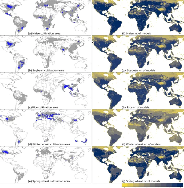
Figure 1. (a–e) Cultivated areas for maize, rice, and soybean from the MIRCA2000 (Monthly Irrigated and Rainfed Crop Areas around the year 2000) dataset (Portmann et al., 2010). Blue indicates grid cells with more that 20 000 ha (10 % of the equatorial grid cell), and the gray contour shows grid cells with more that 10 ha cultivated. Areas for winter and spring wheat areas are adapted from MIRCA2000 and two other sources; see text for details. For irrigated crops, see Fig. S1 in the Supplement. (f–j) Number of models providing simulations for each grid cell. All models provide the minimum areal coverage of the GGCMI Phase 2 protocol, but some provide extra coverage at high latitudes or in arid or otherwise unsuitable areas.
N application to soybeans, which are N fixers and need lit-tle fertilizer. This choice also means that CO2 changes are
applied independently of changes in climate variables, so that higher CO2 is not associated with higher temperatures
or other particular climate changes. The purpose of the ex-periment is not to produce individual scenarios that represent realistic future states but to sample over a wide range of pa-rameter space to enable understanding the factors that drive agricultural changes.
While all CTWN perturbations are applied uniformly across the historical time series, they are applied in different ways. CO2and nitrogen levels are specified as discrete
val-ues applied uniformly over all grid cells. Temperature pertur-bations are applied as absolute offsets from the daily mean, minimum, and maximum temperature time series for each grid cell, and water perturbations are applied as fractional changes to daily precipitation. The irrigated scenario (W∞)
is a particular case of water supply levels, in which crops are assumed to have no water constraints. That is, all crop
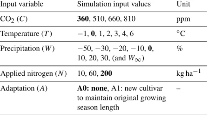
wa-Table 1. GGCMI Phase 2 input parameter levels for each dimen-sion. Temperature and precipitation values indicate the perturba-tions from the historical climatology. Irrigated (W∞) simulations
assume the maximum beneficial levels of water. Bold font indicates the “baseline” or historical level for each dimension. One model provided simulations at the T + 5 level.
Input variable Simulation input values Unit CO2(C) 360, 510, 660, 810 ppm
Temperature (T ) −1, 0, 1, 2, 3, 4, 6 ◦C Precipitation (W ) −50, −30, −20, −10, 0, %
10, 20, 30, (and W∞)
Applied nitrogen (N ) 10, 60, 200 kg ha−1 Adaptation (A) A0: none, A1: new cultivar –
to maintain original growing season length
ter requirements are fulfilled regardless of local water sup-ply limitations. To facilitate comparison, irrigated simula-tions use the same growing seasons as all other simulasimula-tions, even though in reality irrigated growing seasons may be dif-ferent (Portmann et al., 2010), and both irrigated and rainfed cases are simulated with near-global coverage.
The uniform perturbations of the GGCMI Phase 2 proto-col require some care in interpretation. Temperature and pre-cipitation perturbations should be considered as differences from historical climatology within the growing season only. That is, a T + 1 simulation represents a 1◦C warmer grow-ing season, not a 1◦C warmer annual mean temperature. (The distinction is important because in climate projections, win-ters generally warm more than summers; e.g., Haugen et al., 2018.) In the GGCMI Phase 2 protocol, temperature and pre-cipitation perturbations are applied uniformly in space, but future changes in temperature and precipitation will not be spatially or temporally uniform. In a realistic climate pro-jection, higher latitudes generally warm more strongly than lower latitudes (e.g., Hansen et al., 1997), and the northern high latitudes warm more quickly than the southern ones. A GGCMI Phase 2 simulation therefore represents a possible future state that could occur in each grid cell but not one that would in reality occur simultaneously in all grid cells across the globe. The GGCMI Phase 2 simulations are intended to be used for climate impact assessment not directly but in-stead as a “training set” for statistical emulation of each crop model. Once an emulator is constructed from the outputs de-scribed here, it can be driven with growing-season climate anomalies from any climate model projection. The GGCMI Phase 2 protocol does not involve any simulated changes in climate variability, but Franke et al. (2020) demonstrate that these effects are relatively minor and that GGCMI Phase 2 emulators can effectively reproduce crop model yields under realistic future climate scenarios.
The area simulated in the GGCMI Phase 2 protocol ex-tends considerably outside currently cultivated areas, be-cause cultivation may shift under climate change. Figure 1 shows both the present-day cultivated area of rainfed crops (left) and model coverage (right). (Figs. S1–S2 for cur-rently cultivated area for irrigated crops; model coverage is the same.) Each model covers all currently cultivated ar-eas and much of the uncultivated land area, run at 0.5◦ spatial resolution. To reduce the computational burden, the protocol requires simulation over only 80 % of Earth land surface area, omitting areas assumed to remain non-arable even under an extreme climate change, including Greenland, far-northern Canada, Siberia, Antarctica, the Gobi and Sa-hara deserts, and Central Australia. The protocol also al-lows omitting regions judged unsuitable for cropland for non-climatic reasons. Selection criterion involve a combi-nation of soil suitability indices at 10 arcmin resolution and excludes those 0.5◦grid cells in which at least 90 % of the
area is masked as unsuitable according to any single index, and which do not contain any currently cultivated cropland. Currently cultivated areas are provided by the MIRCA2000 (Monthly Irrigated and Rainfed Crop Areas around the year 2000) data product (Portmann et al., 2010). Soil suitability indices measure excess salt, oxygen availability, rooting con-ditions, toxicities, and workability, and are provided by the IIASA (International Institute for Applied Systems Analysis) Global Agro-Ecological Zone model (GAEZ; FAO/IIASA, 2011). The procedure follows that proposed by Pugh et al. (2016). All modeling groups simulate the minimum required coverage, but some provide simulations that extend into masked zones, including, e.g., the Sahara and central Aus-tralia (Fig. 1, right).
2.3 Harmonization between models
The 12 models included in GGCMI Phase 2 are all process-based crop models that are widely used in impacts assess-ments (Table 3). Although some models share a common base (e.g., the LPJ or EPIC families of models), they have subsequently developed independently. Wherever possible, the GGCMI Phase 2 protocol harmonizes inputs, but differ-ences in model structure mean that several key factors cannot be fully standardized across the experiment. These include soil treatment (which affects soil organic matter and carry-over effects of soil moisture across growing years) and base-line climate inputs.
While 10 of the 12 models participating in GGCMI Phase 2 use the AgMERRA historical daily climate data product, two models require subdaily input data and thus use differ-ent baseline climate inputs: Processes of Radiation, Mass and Energy Transfer (PROMET) uses ERA-Interim reanalysis (Dee et al., 2011), and the Joint UK Land Environment Simu-lator (JULES) uses a bias-corrected version of ERA-Interim, the 3 h WFDEI (WATCH Forcing Data ERA-Interim) (Wee-don et al., 2014), specifically the WFDEI version with
pre-cipitation bias-corrected against the Climate Research Unit (CRU) TS3.101/TS3.21 precipitation totals (Harris et al., 2014). The data products show some differences (Figs. S3– S4, which compare data products over currently cultivated areas for each crop). For example, for maize-growing areas, ERA-Interim daily precipitation is biased high from that in AgMERRA by 7 % (< 1σ ), while mean daily precipitation in WFDEI is only 3 % higher. Precipitation differences are largest in wheat areas, where ERA-Interim is substantially wetter (+60 mm yr−1or 10 %). Temperature differences are largest for rice, with ERA-Interim 1◦C cooler than Ag-MERRA, and smaller for other crops, e.g., maize with ERA-Interim 0.45◦C cooler and WFDEI 0.1◦C warmer. These dif-ferences are relatively small compared to the perturbations tested in the protocol.
Planting dates and growing season lengths are standard-ized across models, following the procedure described in El-liott et al. (2015) for the “fullharm” setting. (The exception is that Phase 2, unlike Phase 1, uses identical growing sea-sons for rainfed and irrigated cases, to allow for direct com-parison of simulations along the W dimension.) This harmo-nization is important because the parametrization of growing seasons can have strong effects on simulated yields (Müller et al., 2017; Jägermeyr and Frieler, 2018). In all the GGCMI Phase 2 crop models, sowing dates are prescribed directly, but the length of the growing season is a product of crop phenology, which is driven mostly by phenological param-eters and temperature. Modelers were therefore asked to ad-just their phenological parameters so that the average grow-ing season length of the baseline scenario (C = 360, T = 0, W =0) matched the harmonization target. (The one excep-tion to this harmonizaexcep-tion protocol involves CARbon Assim-ilation In the Biosphere (CARAIB), whose team kept their own growing season specifications rather than tuning to stan-dard lengths.) Two aspects of the procedure should be noted. First, the target growing seasons used in GGCMI Phase 2 are crop and location specific. For example, present-day maize is sown in March in Spain, in July in Indonesia, and in De-cember in Namibia (Portmann et al., 2010). Second, because temperature varies between years in the 30-year baseline cli-matology, realized growing season length will still vary in individual years even after harmonization.
The dependence of harvest dates on climate parameters means that growing seasons will alter under climate change in a model with phenological parameters tuned to match target growing seasons in the baseline climate. In general, warmer future scenarios produce shorter growing seasons. We denote simulations that allow these future changes as “A0” experiments, where 0 denotes “no adaptation”. The GGCMI Phase 2 protocol includes a second set of experi-ments, “A1”, that assume that future cultivars are modified to adjust to changes along the T dimension in the CTWN ex-periment. For these simulations, modelers adjust phenologi-cal parameters for each temperature scenario to hold grow-ing season length approximately constant. (CARAIB
sim-ulations follow the same principle, fixing growing season length at their baseline levels.) That is, the A1 simulations require running a model with seven different choices of cul-tivar parameters, one per warming level. Parameter settings for T = 0 are identical in both A0 and A1. The A1 simula-tions roughly capture the case in which adaptive crop cul-tivar choice ensures that crops reach maturity at roughly the same time as in the current temperature regime. This assump-tion is simplistic, and does not reflect realistic opportunities and limitations to adaptation (Vadez et al., 2012; Challinor et al., 2018) but provides some insight into how crop modi-fications could alter projected impacts on yields and is suffi-ciently easy to implement in a large model intercomparison project as GGCMI.
Growing seasons for maize, rice, and soybean are taken from the SAGE (Center for Sustainability and the Global En-vironment, University of Wisconsin) crop calendar (Sacks et al., 2010), gap filled with the MIRCA2000 crop calen-dar (Portmann et al., 2010) and, if no SAGE or MIRCA2000 data are available, with simulated Lund–Potsdam–Jena man-aged Land (LPJmL) growing seasons (Waha et al., 2012) and are identical to those used in GGCMI Phase 1 (Elliott et al., 2015). In GGCMI Phase 2, we separately treat spring and winter wheat and so must define different growing seasons for each. As for the other crops, we use the SAGE crop cal-endar, which separately specifies spring and winter wheat, as the primary source for 69 % of grid cells. In the remaining areas where no SAGE information is available, we turn to, in order of preference, the MIRCA2000 crop calendar (Port-mann et al., 2010) and to simulated LPJmL growing seasons (Waha et al., 2012). These datasets each provide several op-tions for wheat growing season for each grid cell but do not label them as spring or winter wheat. We assign a growing season to each wheat type for each location based on its base-line climate conditions. A growing season is assigned to win-ter wheat if all of the following hold, and to spring wheat otherwise:
– The monthly mean temperature is below freezing point (< 0◦C) at most for 5 months per year (i.e., winter is not too long).
– The coldest 3 months of a year are below 10◦C (i.e.,
there is a winter).
– The season start date fits the criteria that
– if in the Northern Hemisphere, it is after the warmest or before the coldest month of the year (as winter is around the end/beginning of the calendar year);
– if in the Southern Hemisphere, it is after the warmest and before the coldest month of the year (as winter is in the middle of the calendar year). Nitrogen (N) application is standardized in timing across models. N fertilizer is applied in two doses, as is often the
norm in actual practice, to reduce losses to the environment. In the GGCMI Phase 2 protocol, half of the total fertilizer input is applied at sowing and the other half on day 40 af-ter sowing, for all crops except for winaf-ter wheat. For winaf-ter wheat, in practice the application date for the second N fer-tilizer application varies according to local temperature, be-cause the length of winter dormancy can vary strongly. In the GGCMI Phase 2 protocol, the second fertilization date for winter wheat must lie at least 40 d after planting and – if not contradicting the distance to planting – no later than 50 d be-fore maturity. If those limits permit, the second fertilization is set to the middle day of the first month after sowing that has average temperatures above 8◦C.
All stresses in models are disabled other than those related to nitrogen, temperature, and water. For example, model re-sponses to alkalinity, salinity, and non-nitrogen nutrients are all disabled. No other external N inputs are permitted – that is, there is no atmospheric deposition of nitrogen – but some models allow additional release of plant-available ni-trogen through mineralization in soils. In LPJmL, the Lund– Potsdam–Jena General Ecosystem Simulator (LPJ-GUESS), and Agricultural Production Systems sIMulator (APSIM), soil mineralization is a part of model treatments of soil or-ganic matter and cannot be disabled. Some additional differ-ences in model structure mean that several key factors are not standardized across the experiment. For example, carryover effects across growing years including residue management and soil moisture are treated differently across models. 2.4 Output data products
All models in GGCMI Phase 2 provide 30-year time series of annual crop yields for each scenario, 0.5◦grid cell and crop,
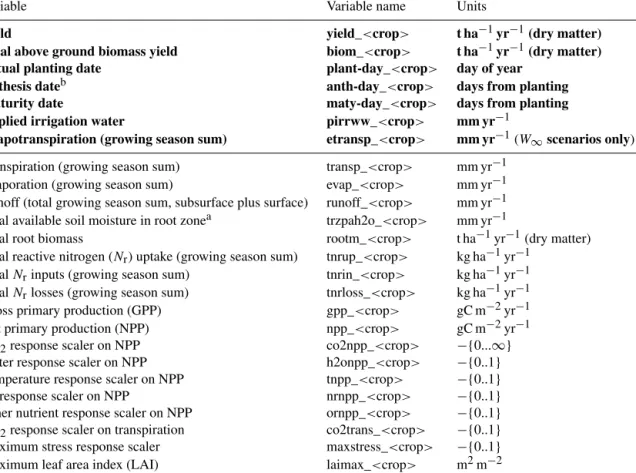
in units of t ha−1yr−1. They also provide all available vari-ables of the following six: total aboveground biomass yield; the dates of planting, anthesis and maturity; applied irriga-tion water in irrigated scenarios; and total evapotranspira-tion. We term these seven variables the “mandatory” outputs, but note that some models do not compute all of them; e.g., CARAIB does not compute the anthesis date. Besides these seven “mandatory” data products (Table 2, bold), the proto-col requests any or all of 18 “optional” additional output vari-ables (Table 2, plain text). Participating modeling groups pro-vided between 3 (PEPIC) and 18 (APSIM-UGOE) of these optional variables.
All output data are supplied as NetCDF version 4 files, each containing values for one variable in a 30-year time series associated with a single scenario, for all grid cells. Filenames follow the naming conventions of GGCMI Phase 1 (Elliott et al., 2015), which themselves are derived from those of ISIMIP (Frieler et al., 2017). Filenames are spec-ified as [model]_[climate]_hist_fullharm_[variable]_[crop]
_global_annual_[start-year]_[end-year]_[C]]_[T]_[W]_[N]_[A].nc4 Here, [model] is the crop model name; [climate] is the original climate input
dataset (typically AgMERRA); [variable] is the output variable (of those in Table 2); [crop] is the crop abbrevi-ation (“mai” for maize, “ric” for rice, “soy” for soybean, “swh” for spring wheat, and “wwh” for winter wheat); and [start-year] and [end-year] specify the first and last years recorded on file. [C], [T ], [W ], [N ], and [A] indicate the CTWN-A settings, each represented with the respective uppercase letter and the number indicating the level (e.g., “C360_T0_W0_N200”; see Table 1). Except for the CTWN-A letters, the entire filename needs to be in small caps. All filenames include the identifiers global and annual to distinguish them as global, annual model output, following the updated ISIMIP file naming convention (Frieler et al., 2017).
Output data are provided on a regular geographic grid, identical for all models. Grid cell centers span latitudes from −89.75 to 89.75◦and longitudes from −179.75 to 179.75◦.
Missing values where no crop growth has been simulated are distinguished from crop failures: a crop failure is reported as zero yield but non-simulated areas (including ocean grid cells) have yields reported as “missing values” (defined as 1 × 10²⁰in the NetCDF files). Following NetCDF standards, latitude, longitude, and time are included as separate vari-ables in ascending order, with units “degrees north”, “degrees east”, and “growing seasons since 1 January 1980 00:00:00”. Following GGCMI Phase 1 standards, the first entry in each file describes the first complete cropping cycle simu-lated from the given climate input time series. In the Ag-MERRA time series used for GGCMI Phase 2, the first year provided is 1980 but the date of the first entry can vary by crop and location. In the Northern Hemisphere, for summer crops like maize (sown in spring 1980 and harvested in fall 1980), the first harvest record would be of 1980, but for win-ter wheat (sown in fall 1980 and harvested in spring 1981) the first harvest record would be of 1981. Output files report the sequence of growing periods rather than calendar years. While there is generally one sowing event per calendar year (since simulations with harmonized growing seasons do not permit double cropping), in some cases harvest events may skip or repeat within a calendar year. For example, because soybeans in North Carolina are typically harvested well into December, some calendar years may include no harvest (if it is not completed until after 31 December) or two harvests (one in January and one 11 months later in the following De-cember).
3 Models contributing
The 12 models participating in GGCMI Phase 2 are listed in Table 3. Models differ substantially in structure and param-eterization and can be separated into two broad categories: site-based (field-scale) models and global ecosystem mod-els. The six site-based models are APSIM, pDSSAT, and the EPIC family of models; the six ecosystem models are
Table 2. Output variables, naming convention, and units in the GGCMI Phase 2 protocol. Items in bold text are the mandatory minimum requirements (if model capacities allow for these outputs). Other variables are optionally provided depending on availability and participating modeling groups provided between 3 (PEPIC) and 18 (APSIM-UGOE) of these optional variables.
Variable Variable name Units
Yield yield_<crop> t ha−1yr−1(dry matter) Total above ground biomass yield biom_<crop> t ha−1yr−1(dry matter) Actual planting date plant-day_<crop> day of year
Anthesis dateb anth-day_<crop> days from planting Maturity date maty-day_<crop> days from planting Applied irrigation water pirrww_<crop> mm yr−1
Evapotranspiration (growing season sum) etransp_<crop> mm yr−1(W∞scenarios only)
Transpiration (growing season sum) transp_<crop> mm yr−1 Evaporation (growing season sum) evap_<crop> mm yr−1 Runoff (total growing season sum, subsurface plus surface) runoff_<crop> mm yr−1 Total available soil moisture in root zonea trzpah2o_<crop> mm yr−1
Total root biomass rootm_<crop> t ha−1yr−1(dry matter) Total reactive nitrogen (Nr) uptake (growing season sum) tnrup_<crop> kg ha−1yr−1
Total Nrinputs (growing season sum) tnrin_<crop> kg ha−1yr−1
Total Nrlosses (growing season sum) tnrloss_<crop> kg ha−1yr−1
Gross primary production (GPP) gpp_<crop> gC m−2yr−1 Net primary production (NPP) npp_<crop> gC m−2yr−1 CO2response scaler on NPP co2npp_<crop> −{0...∞}
Water response scaler on NPP h2onpp_<crop> −{0..1} Temperature response scaler on NPP tnpp_<crop> −{0..1} Nrresponse scaler on NPP nrnpp_<crop> −{0..1}
Other nutrient response scaler on NPP ornpp_<crop> −{0..1} CO2response scaler on transpiration co2trans_<crop> −{0..1} Maximum stress response scaler maxstress_<crop> −{0..1} Maximum leaf area index (LAI) laimax_<crop> m2m−2
aGrowing season sum, basis for computing average soil moisture.bProvided where possible.
LPJmL, LPJ-GUESS, PROMET, CARAIB, Organising Car-bon and Hydrology In Dynamic Ecosystems (ORCHIDEE), and JULES. Models employ a variety of approaches for the core modules such as primary production or evapotranspira-tion. For primary production, site-based models employ light use efficiency approaches and ecosystem models use pho-tosynthesis approaches. For evapotranspiration, most mod-els use Priestley–Taylor, Penman–Monteith or Hargreaves schemes, but JULES and PROMET utilize a land surface model approach instead. Note that models that share a com-mon genealogy may still use different schemes for evapotran-spiration: for example, EPIC-TAMU uses Penman–Monteith and EPIC-IIASA uses Hargreaves. To describe soils, most models use either the Harmonized World Soil Database (HWSD) from the FAO (FAO/IIASA/ISRIC/ISSCAS/JRC, 2012) or the ISRIC-WISE database (Batjes, 2005) or a derivation thereof. Table S1 in the Supplement provides de-tails on these model characteristics as well as on implemen-tation, including spin-up, calibration other than growing sea-son, residue management, and irrigation rules.
Table 3 also describes the simulation output contribution of each model to the GGCMI Phase 2 archive. Not all mod-eling groups provided simulations for the full protocol de-scribed above. Given the substantial computational require-ments, different participation tiers were specified to allow submission of smaller subsets of the full protocol. These sub-sets were designed as alternate samples across the four di-mensions of the CTWN space, with full (12) and low (4) op-tions for the C · N variables, and full (63), reduced (31), and minimum(9) options for T · W variables (described below). All participating modeling groups provided identical cover-age of the CTWN parameter space for different crops, but most differed in CTWN coverage of A0 and A1 scenarios. Since the adaptation dimension was defined as a secondary priority for GGCMI Phase 2, some models provided a more limited set of A1 scenarios. Of these, EPIC-IIASA, JULES, and ORCHIDEE-crop provided no A1 scenarios.
The different participation levels are defined by combining the C · N sets with the T · W sets:
– full: all 756 A0 simulations (all 12 C × N * all 63 T × W);
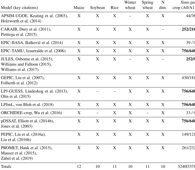
Table 3. Models included in GGCMI Phase 2 and the number of CTWN-A simulations performed. The maximum number is 756 for A0 (no adaptation) experiments, and 648 for A1 (maintaining growing length) experiments, since T0 is not simulated under A1. “N dim” indicates whether the models are able to represent varying nitrogen levels. Each model provides the same set of CTWN simulations across all its modeled crops, but some models omit individual crops. (For example, APSIM-UGOE does not simulate winter wheat.) Bold numbers indicate those models that provided all specified simulations (with or without varying nitrogen).
Winter Spring N Sims per Model (key citations) Maize Soybean Rice wheat wheat dim. crop (A0/A1) APSIM-UGOE, Keating et al. (2003),
Holzworth et al. (2014)
X X X – X X 44/36
CARAIB, Dury et al. (2011), Pirttioja et al. (2015)
X X X X X – 252/216
EPIC-IIASA, Balkoviˇc et al. (2014) X X X X X X 39 / 0 EPIC-TAMU, Izaurralde et al. (2006) X X X X X X 756/648 JULES, Osborne et al. (2015),
Williams and Falloon (2015), Williams et al. (2017)
X X X – X – 252/0
GEPIC, Liu et al. (2007), Folberth et al. (2012)
X X X X X X 430/181
LPJ-GUESS, Lindeskog et al. (2013), Olin et al. (2015)
X – – X X X 756/648
LPJmL, von Bloh et al. (2018) X X X X X X 756/648 ORCHIDEE-crop, Wu et al. (2016) X – X X – X 33 / 0 pDSSAT, Elliott et al. (2014b),
Jones et al. (2003)
X X X X X X 756/648
PEPIC, Liu et al. (2016a), Liu et al. (2016b)
X X X X X X 149/121
PROMET, Hank et al. (2015), Mauser et al. (2015), Zabel et al. (2019)
X X X X X X 261/232
Totals 12 10 11 10 11 10 5240|3378
– high: 362 simulations (all 12 C × N combinations · re-ducedT × W set of 31 combinations);
– mid: 124 simulations (low 4 C × N combinations · re-ducedT × W set of 31 combinations); and
– low: 36 simulations (low 4 C × N combinations · mini-mumT × W set of 9 combinations).
Of the 12 models submitting data, six followed the full pro-tocol; these are marked with bold text in the last column of Table 3. However, note that two of these models (CARAIB and JULES) cannot represent nitrogen effects explicitly and so do not sample over the nitrogen dimension. Two models followed high with minor modifications (GEPIC adding an additional T level and PROMET omitting the intermediate N level). One model (PEPIC) followed mid but included an ad-ditional C level. Three models approximately followed low
with APSIM-UGOE and EPIC-IIASA providing some ad-ditional T × W levels and ORCHIDEE-crop omitting some T × W combinations.
The combinations of perturbation values in the C × N and T ×Wparameter spaces used in the various participation lev-els are chosen to provide maximum coverage over plausible future values. For the C × N space, we specify
– full as 12 pairs, with four C values (360, 510, 660, 810 ppm) and three N values (10, 60, 200 kg ha−1yr−1) and
– low as only four pairs: C360_N10, C360_N200,
C660_N60, and C810_N200.
For the T × W space, we specify
– reduced as 31 alternating combinations, with different Ws for even Ts than for odd Ts. For even Ts (i.e., T0,
T2, T4, T6), we use W = −50, −20, 0, +30 = 4 · 4 = 16
pairs. For odd Ts (i.e., T −1, T 1, T 3), we use W = −30, −10, +10, +30, inf = 3 · 5 = 15 pairs;
– minimum as nine combinations: T−1W−10, T0W10,
T1W−30, T2W−50, T2W20, T3W30, T4W0, T4Winf,
T6W−20.
4 Results
To illustrate the properties of the GGCMI Phase 2 model sim-ulations, we provide an evaluation of model performance by comparing model and historical yields, and show example results that demonstrate the spread of model responses to cli-mate and management inputs.
4.1 Evaluation of model performance
All models participating in GGCMI Phase 2 have be evalu-ated against historical yields and site-specific experimental data. Most models (9 of 12, all but CARAIB, JULES, and PROMET) have been evaluated in their global setup in the GGCMI Phase 1 evaluation exercise (Müller et al., 2017), and many have used the GGCMI Phase 1 online tool to sim-ilarly evaluate subsequent model versions (e.g., von Bloh et al., 2018). Evaluating the performance of crop models in the GGCMI Phase 2 archive is complicated by the artificial nature of the protocol: the settings in the CTWN-A experi-ment design do not reflect actual conditions in the real world. The protocol includes one scenario of near-historical climate inputs (T0, W0, C360), but the prescribed uniform nitrogen
application levels do not reflect real-world fertilizer prac-tices. Models also omit detailed calibrations to reflect the performance of historical cultivars.
We provide a partial evaluation of the models’ skill in reproducing crop yield characteristics using the methodol-ogy of Müller et al. (2017), developed for GGCMI Phase 1. Müller et al. (2017) evaluate how well model crop yield responses in a historical run capture real-world yield vari-ations driven by year-to-year temperature and precipitation variations. Following this approach, we compare yields in the GGCMI Phase 2 baseline simulations with detrended his-torical yields from the Food and Agriculture Organization of the United Nations (FAO, 2018) by calculating the Pear-son product moment correlation coefficient over 26 years of yield. The procedure is sensitive to the detrending method and the area mask used to aggregate yields; we use a 5-year running mean removal and the MIRCA2000 cultivation area mask for aggregation. In some cases, the model time series are shifted by 1 year to account for discrepancies in FAO or model year reporting. Because the GGCMI Phase 2 proto-col imposes fixed, uniform nitrogen application levels that are not realistic for individual countries, we evaluate control
runs for each model at multiple N levels whenever possible. Overall, nine of the GGCMI Phase 2 models (Table 3) pro-vide historical runs for all three nitrogen levels (10, 60, and 200 kg ha−1yr−1).
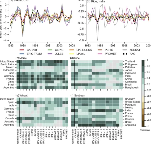
As expected due to the unrealistic features described above, correlation coefficients for the GGCMI Phase 2 sim-ulations are slightly lower than those found in the Phase 1 evaluation, but models show reasonable fidelity at capturing year-to-year variation (Fig. 2). For example, global correla-tion coefficients in Phase 1 and Phase 2, respectively, are 0.89 and 0.74 for maize, 0.67 and 0.64 for wheat, and 0.64 and 0.59 for soybeans. (Phase 1 values are from Figs. 1–4 and 6 in Müller et al., 2017.) Differences in fidelity between re-gions and crops exceed differences between models; that is, Fig. 2c–f show more color similarity in horizontal than ver-tical bars. For example, maize in the United States is consis-tently well simulated, while maize in Indonesia is problem-atic (mean Pearson correlation coefficients of 0.68 and 0.18, respectively). Note that in this methodology, simulations of crops with low year-to-year variability such as irrigated rice and wheat will tend to score more poorly than those with higher variability. In some cases, especially in the develop-ing world, low correlation coefficients may point to report-ing problems in the FAO statistics and to real-world variabil-ity caused by variations in management rather than weather (Ray et al., 2012; Müller et al., 2017). No single model con-sistently exhibits greater fidelity than others. Instead, each model shows near best-in-class performance for at least one location–crop combination. For example, pDSSAT is the best model for maize in the US, LPJmL and GEPIC are best in Germany, PROMET is best in Argentina, and PEPIC and LPJ-GUESS are best in France.
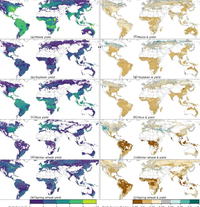
4.2 Model crop yield responses under CTWN forcing Crop models in the GGCMI Phase 2 ensemble show broadly consistent responses to climate and management perturba-tions in most regions, with a strong negative impact of in-creased temperature in all but the coldest regions. Mapping the distribution of baseline yields and yield changes shows the geographic dependencies that underlie these results. Ab-solute yield potentials show strong spatial variation, with much of the Earth’s surface area unsuitable for any of these crops (Fig. 3, left). Crop yield changes under climate pertur-bations also show distinct geographic patterns (Fig. 3, right, which shows fractional yield differences between the base-line and T + 4 A0 scenarios). In general, models agree most on yield response in regions where yield potentials are cur-rently high and therefore where crops are curcur-rently grown. In A0 simulations, models show robust decreases in yields at low latitudes, and highly uncertain ensemble mean increases at most high latitudes. Low-latitude yield reductions are due in part to shortening of the growing season under warming and in part to the direct effects of higher temperature. In A1 simulations, where growing seasons length does not change,
Figure 2. Assessment of crop model performance in GGCMI Phase 2, following the protocol of GGCMI Phase 1 (Müller et al., 2017). (a, b) Example time series comparison between simulated crop yield and FAO country statistics (FAO, 2018) at the country level for two example high production countries: US maize and rice in India, both for the 200 kg ha−1nitrogen application level. (c–f) Heatmaps illustrating the Pearson r correlation coefficient between the detrended simulated and observed country-level mean yields for the top 10 countries by production for each crop, of those countries with continuous FAO data over 1981–2010. We show separate comparisons for simulations with the three different nitrogen application levels, denoted 1, 2, and 3 for 10, 60, and 200 kg N ha−1, respectively. Panels (a, c, e) show correlation of ensemble mean yields with FAO data. Because FAO does not distinguish between wheat types, we sum simulated spring and winter wheat for models that provide both (see Table 3). Note that differences by region and crop are stronger than difference between models; e.g., horizontal bars are more similar in color than vertical bars. Countries are ordered alphabetically, not by production quantity.
temperature-related reductions in yield are more muted (see Fig. S14). In both A0 and A1 simulations, models show some increases in high mountain regions that are currently cold limited.
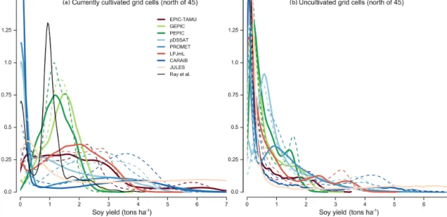
Projections of strong yield growth at higher latitudes should be treated with caution, since the effects evident in Fig. 3 are due in part to inaccuracies in model representa-tions of present-day crop yields. For example, at latitudes north of 45◦, the GGCMI Phase 2 models collectively sug-gest strong (but uncertain) growth in soybean yields under
warmer conditions (Fig. 3g). However, model differences are greater in the baseline than future simulations and greatest in currently cultivated areas (Fig. 4). Both the mean pro-jected growth and the inter-model spread are driven by three models that show almost zero present-day potential soybean yields across the entire high-latitude region, even in locations where soybeans are currently grown (Fig. 4, left). PROMET, for example, involves a stronger response to cold than other models (e.g., LPJmL) with frost below −8◦C irreversibly killing non-winter crops and prolonged periods of
below-Figure 3. Illustration of the spatial patterns of baseline yields (a–e) and yield changes (f–j) in the GGCMI Phase 2 ensemble. The left column shows multi-model climatological (30-year) median yields for the baseline scenario, with white stippling indicating areas where these crops are not currently cultivated. Areas with less than 0.5 t ha−1in the baseline are masked. Absence of cultivation aligns well with the lowest yield contour (0–2 t ha−1). The right column shows multi-model mean fractional yield changes in the T + 4◦C scenario relative to the baseline scenario. Areas without stippling are those where models agree on changes: the multi-model mean fractional change exceeds the standard deviation of changes in individual models. Stippling indicates areas of low confidence (1 < 1σ ). Some spatial structure in projected changes at high latitudes may be due to differences in model coverage; see Fig. 1.
optimum temperatures also leading to complete crop fail-ure. Over the high-latitude regions simulated by both models, 52 % of grid cells in PROMET report 0 yield in the present climate vs. 11 % of cells in the T + 4 scenario, leading to a strong yield gain in warmer future climates. In LPJmL out-puts, the same high-latitude area is deemed suitable for cul-tivation even in baseline climate, with crop failure rates of 4 % and 5 % in present and T + 4 cases, so that projected yield changes are modest (Fig. 4). These spurious low
base-line yields result in very large fractional changes in the T + 4 warming scenario, when all models agree that conditions be-come favorable for soybeans. Those models that most accu-rately reproduce present-day high-latitude soybean yields of 1–2 t ha−1 (Ray et al., 2012) in fact show a slight decrease in yield under a warming scenario (Fig. 4a). Apparent future yield increases in the multi-model mean are driven by the least realistic simulations.
Figure 4. Model probability densities for soybean yields at latitudes north of 45◦in historical and warming simulations in the A0 case. While 10 GGCMI Phase 2 models provide simulations (Table 3); we show eight representative models for clarity. Probability density functions are estimated separately for locations with some current cultivation (a, approximately 2500 grid cells, unweighted by cultivated area) and for uncultivated locations (b, approximately 1500 grid cells), for baseline historical (solid) and T + 4 (◦C) (dashed) simulations. Black line in panel (a) shows actual yields from 1997 to 2003 derived from Ray et al. (2012). For historical simulations, models agree on low potential yields in currently uncultivated areas (b) but disagree widely on yields in currently cultivated areas (a). Color code groups models into those with realistic yield distributions peaking at 1–2 t ha−1(green), those with flatter distributions extending to unrealistically high values (red), and those with predominantly zero yields (blue). “Green” models show slight decreases under T + 4 warming, “red” models moderate increases, and “blue” models large increases.
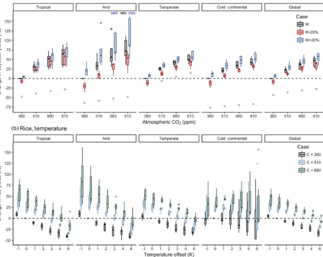
The GGCMI Phase 2 exercise offers the opportunity to examine and characterize not just crop response to a single temperature change but nonlinearities in responses and in-teractions between factors. We illustrate a few of these rela-tionships in Figs. 5–6 using A0 simulations to capture max-imum climate effects. We choose crops and factors whose effects are reasonably well understood and show that these are reproduced in models. It is expected, for instance, that increases in precipitation should buffer the effects of warmer temperatures and that CO2increases should reduce damage
to crops in scenarios where water is limited. Models gener-ally confirm expected behavior but also provide insight into unforeseen interactions. To show geographic effects, we di-vide model responses in Figs. 5–6 by the primary Köppen– Geiger climate regions (Rubel and Kottek, 2010), showing the yield changes across all simulated grid cells in each re-gion. In each panel, we examine relationships between two factors, showing yield response against one for several sce-narios of the other, in box plots that show the inter-model spread. The responses highlighted here are qualitatively sim-ilar across all crops included in this study (Figs. S5–S9 for all simulated area and S10–S13 for cultivated area only).
For all crops, warming scenarios with precipitation held constant produce yield decreases in most regions. These im-pacts are robust for even moderate climate perturbations. For rainfed maize, even a 1◦C temperature increase with other
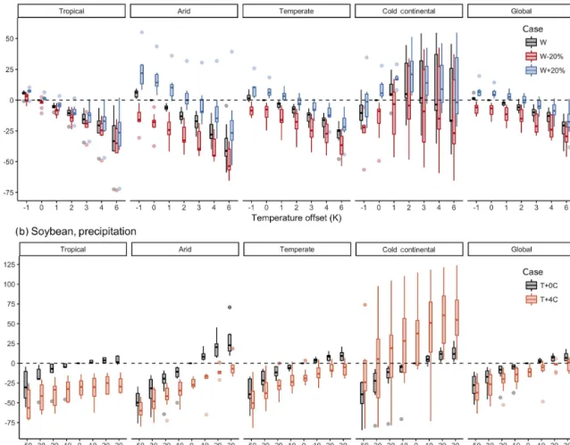
factors held constant produces a median regional decline in potential yield that exceeds the variance across models, in all but the “cold-continental” regions (Fig. 5a). The remain-ing areas (“warm temperate”, “equatorial”, and “arid”) ac-count for nearly three-quarters of global maize production. In the high-latitude “cold-continental” region, potential yield changes are positive but highly uncertain, for the reasons discussed previously; uncertainties are larger even for maize than for soybeans. (Compare Fig. 5a and b.) Temperature ef-fects are somewhat nonlinear, with the largest impacts for maize in the warm “tropical” region (for soybeans, tempera-ture effects are more complex; see Fig. S5). Precipitation ef-fects on rainfed crops are more strongly nonlinear. The cur-vature of the precipitation response can be seen by eye in Fig. 5b: soybean yields are strongly negatively impacted by reduced rainfall, peak under increased precipitation of 20 %, and actually decline at higher precipitation levels.
As expected, precipitation and temperature effects inter-act, with increases in precipitation buffering yield responses to temperature. Increased rainfall mitigates the negative im-pacts of warmer temperatures caused by increased evapotran-spiration (e.g., Allen et al., 1998). For maize, the effect is relatively modest outside the “arid” regions (Fig. 5a). Glob-ally, a 4◦C temperature rise with no change in precipitation results in median loss of ∼ 13 % of rainfed maize, with all models showing a negative response. With a 20 % increase in
Figure 5. Illustration of the distribution of regional yield changes across the multi-model ensemble, split by Köppen–Geiger climate regions, and with global response in rightmost panel. The y axis is the fractional change in the regional average climatological (30-year mean) potential yield relative to the baseline. Box-and-whisker plots show distribution across models, with median marked; edges are first and third quartiles and whiskers extend to 1.5 · IQR. The figure shows all simulated grid cells for each model; see Figs. S10–S13 for only currently cultivated land. We highlight responses to individual factors; note that results are not directly comparable to simulations of realistic projected climate scenarios with identical global mean changes. Models generally agree outside high-latitude regions, with projected changes exceeding inter-model variance. (a) Response of rainfed maize to applied uniform temperature perturbations, for three discrete precipitation perturbation levels (−20 %, 0 %, and +20 %), with CO2and nitrogen held constant at baseline values (360 pmm and 200 kg ha−1yr−1). Outliers in the
tropics (strong negative impact of higher T ) are the pDSSAT model; outliers in the arid region (strong positive impact of higher P ) are JULES. (b) Response of rainfed soybeans to applied uniform precipitation perturbations, for two discrete temperature levels. Cases with reduced precipitation show greater inter-model spread than those with increased precipitation. At very large precipitation increases, yield changes level out: benefits saturate once water availability is no longer limiting. Precipitation changes are more important in the arid region, as expected. Note the large uncertainty in the cold continental region, also illustrated in Figs. 3 and 4.
precipitation, the median yield loss is ∼ 8 %. For soybeans, the equivalent values are ∼ 11 % and 1 %, respectively. De-creased rainfall, on the other hand, amplifies yield losses and also increases inter-model variance. That is, models agree that the response to decreased water availability is negative in sign but disagree on its magnitude. Outside of arid regions, the interaction effect itself shows little nonlinearity (i.e., re-sponse slopes in Fig. 5a and b are roughly parallel). As ex-pected, irrigated crops are more resilient to temperature in-creases in all regions, especially so where water is already limiting (other than winter wheat; Fig. S9).
Increased CO2 boosts yields overall through the
well-known CO2 fertilization effect (Fig. 6). The effect is
strongest for the C3 crops (wheat, soybeans, and rice), while maize, a C4 grass, has a comparatively muted response. We show irrigated rice and rainfed soy in Fig. 6 as representative C3 crops. The effect of CO2on yields is nonlinear, as
ex-pected, with significant benefit from small increases but with effects plateauing at higher concentrations (Fig. 6). CO2and
temperature effects show minimal interaction. This effect is seen in Fig. 6a, which shows nearly parallel response slopes at different CO2levels. That is, CO2fertilization does little to
Figure 6. Illustration of the distribution of regional yield changes across the multi-model ensemble, here for soybeans and rice for the A0 case. Conventions are as in Fig. 5. (a) Response of rainfed soybeans to atmospheric CO2, for three discrete precipitation perturbation levels
with temperature and nitrogen held constant at baseline values. Low outliers are the EPIC-TAMU model and the high outliers in the arid region are the JULES model. Reduced precipitation tends to steepen the CO2response and increased precipitation tends to flatten it, as
expected. Reduced precipitation tends to increase the inter model spread, especially at the highest CO2levels. (b) Response of irrigated
rice for three discrete CO2levels, with nitrogen and precipitation held constant. CO2does not change the nature of temperature response
respective to baseline as the slopes at each CO2level are relatively constant.
change the nature of the temperature response. On the other hand, CO2and precipitation effects interact strongly, as
ex-pected since higher CO2levels allow reduced stomatal
con-ductance and evapotranspiration losses, mitigating the effect of reduced rainfall (e.g., McGrath and Lobell, 2013). This interaction is seen in Fig. 6b as smaller yield losses from re-duced rainfall when CO2levels are higher. For example, for
soy, raising CO2 to 510 ppm actually outweighs the
multi-model median damages caused by a 20 % precipitation re-duction in all climate regions. All crops show similar behav-ior, but note that model uncertainties for wheat are substan-tially higher than those for other crops. (Compare Fig. 6a for soy and Fig. S7 for wheat.)
We show some additional cases in the Supplement. As noted previously, the A1 adaptation simulations involve sig-nificantly moderated temperature impacts relative to the A0 simulations shown here (Fig. S14). Figures S15 and S16
show the response in the nitrogen dimension and an irriga-tion water demand response example.
5 Discussion and conclusions
The GGCMI Phase 2 experiment provides a database de-signed to allow detailed study of crop yields in process-based models under climate change. While previous crop model in-tercomparison projects in the climate change context have focused on simulations along realistic projected climate sce-narios (e.g., Rosenzweig et al., 2014), the use of systematic input parameter variations in GGCMI Phase 2, with up to 756 scenarios, allows not only comparing yield sensitivities to changing climate and management inputs but also evaluat-ing the complex interactions between important drivevaluat-ing fac-tors: CO2, temperature, water supply, and applied nitrogen.
The global extent of the experiment also allows identifying geographic shifts in high potential yield locations. With 12 participating models and 31 simulation years per scenario, the complete database constitutes over 150 000 years of grid-ded global yield simulation output for each crop.
Preliminary results shown here highlight some of the in-sights facilitated by the simulation exercise and lend con-fidence in the models. In validation tests of historical sim-ulations, year-to-year correlations in modeled and actual country-level yields are similar to those of GGCMI Phase 1. In simulations of scenarios with perturbed climate and man-agement factors, models broadly agree on changes outside the high latitudes, with the magnitude of changes at nearly all perturbation levels exceeding the inter-model spread. At high latitudes, differences between models may result from differences in their assumed yields in current cold conditions. In simulations with multiple perturbations, interactions be-tween major yield drivers (e.g., temperature and precipitation in Fig. 5, or precipitation and CO2in Fig. 6) generally follow
expectations and produce physically reasonable responses in crop yields.
Users should however be aware of some limitations of the GGCMI Phase 2 experiment that affect its potential ap-plications. First, absolute yield values in the baseline sce-nario, driven by 1981–2010 historical climate, will gener-ally not match observed yields over this time period. In order to match current yields, process-based models must be re-tuned to account for the constant evolution of crop cultivar genetics and management practice (e.g., Jones et al., 2017). GGCMI Phase 2 is intended as a study of model responses to changes in climatic conditions, which are assumed insen-sitive to the adjustments needed to reproduce present-day yields. The baseline scenario also includes no trend in CO2,
and no individual case involves realistic country-specific ni-trogen application levels (Elliott et al., 2015).
The second major caveat is that no individual GGCMI Phase 2 simulation is itself a realistic future yield projection. The uniform applied offsets in temperature and precipitation sample over potential changes, and do not individually cap-ture the spatially heterogeneous warming and precipitation changes expected in realistic climate projections. GGCMI Phase 2 simulation results can be used for impacts projection but only with the construction of an emulator of crop yield re-sponse to climatological changes, which can then be driven by arbitrary climate scenarios. Such emulators are shown to accurately reproduce crop model output under realistic cli-mate projections, even though the GGCMI Phase 2 experi-ment does not sample over potential changes in the higher-order moments in temperature and precipitation distributions (Franke et al., 2020). Note that some factors that may af-fect future climate-driven yield impacts cannot be captured by the GGCMI Phase 2 models in any usage, since models do not include representations of pests, diseases, and weeds. Offline crop model simulations (i.e., with prescribed rather than dynamically simulated atmospheric conditions) can also
not capture any feedbacks on the climate from land use, such as irrigation impacts on humidity (e.g., Decker et al., 2017).
We expect that the GGCMI Phase 2 simulations will yield multiple insights in future studies. Potential applications in-clude, as mentioned, the construction of emulators and yield response surfaces that can be used for both model diagnosis and impacts assessment. Specific studies could include ana-lyzing the drivers of temperature-related yield losses (which may be due to both direct thermal effects or to shortening growing seasons); the benefits of adaptation; interactions be-tween CO2and water or other CTWN factors affecting yield;
changes in nitrogen use efficiency; geographic shifts in re-gional production; and rere-gional differences in yield sensitiv-ities to CTWN-A factors. Emulators based on the dataset can be used to identify hotspots of crop system vulnerability and to conduct rapid assessment of new climate projections. In general, the development of multi-model ensembles involv-ing systematic parameter sweeps has large promise both for increasing understanding of potential future crop responses and for improving process-based crop models.
Code and data availability. All input data are available via zenodo at https://doi.org/10.5281/zenodo.3773827 (Müller et al., 2020). For the minimum cropland mask, choose the boolean_cropmask_ggcmi_phase2.nc4 file. Growing period data for wheat are now divided up into winter and spring wheat, whereas all other growing season data (maize, rice, soybean) are the same as in Phase 1.
Supplement. The supplement related to this article is available on-line at: https://doi.org/10.5194/gmd-13-2315-2020-supplement.
Author contributions. JE, CM, and ACR designed the research. CM, JJ, JB, PC, MD, PF, CF, LF, MH, RCI, IJ, CJ, NK, MK, WL, SO, MP, TAMP, AR, XW, KW, and FZ performed the sim-ulations. JF, JJ, CM, and EM performed the analysis, and JF, EM, and CM prepared the manuscript. All authors contributed to editing the manuscript.
Competing interests. The authors declare that they have no conflict of interest.
Acknowledgements. This research was performed as part of the Center for Robust Decision-making on Climate and Energy Policy (RDCEP) at the University of Chicago. This is paper number 35 of the Birmingham Institute of Forest Research. Computing resources were provided by the University of Chicago Research Computing Center (RCC). We thank two anonymous reviewers for their helpful comments.
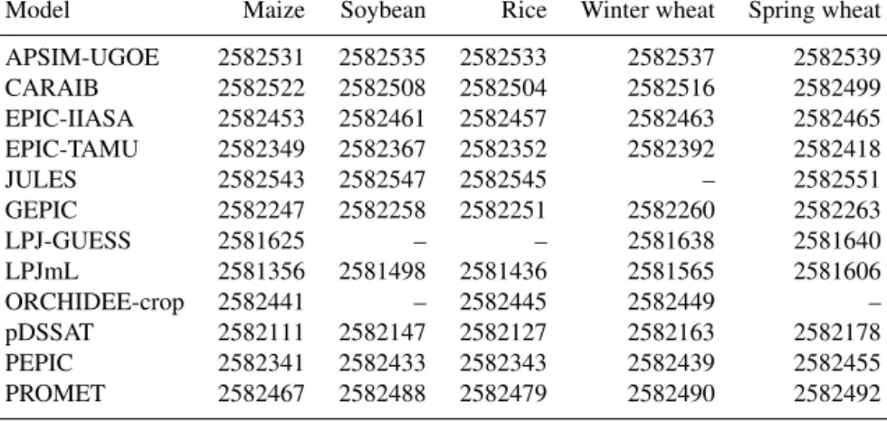
Table 4. DOIs for model data outputs. All model output data can be found at https://doi.org/10.5281/zenodo/XX, where XX is the value listed in the table.
Model Maize Soybean Rice Winter wheat Spring wheat APSIM-UGOE 2582531 2582535 2582533 2582537 2582539 CARAIB 2582522 2582508 2582504 2582516 2582499 EPIC-IIASA 2582453 2582461 2582457 2582463 2582465 EPIC-TAMU 2582349 2582367 2582352 2582392 2582418 JULES 2582543 2582547 2582545 – 2582551 GEPIC 2582247 2582258 2582251 2582260 2582263 LPJ-GUESS 2581625 – – 2581638 2581640 LPJmL 2581356 2581498 2581436 2581565 2581606 ORCHIDEE-crop 2582441 – 2582445 2582449 – pDSSAT 2582111 2582147 2582127 2582163 2582178 PEPIC 2582341 2582433 2582343 2582439 2582455 PROMET 2582467 2582488 2582479 2582490 2582492
Financial support. RDCEP is funded by NSF (grant no. SES-1463644) through the Decision Making Under Uncertainty pro-gram. James Franke was supported by the NSF NRT program (grant no. DGE-1735359) and the NSF Graduate Research Fellowship Program (grant no. DGE-1746045). Christoph Müller was sup-ported by the MACMIT project (grant no. 01LN1317A) funded through the German Federal Ministry of Education and Research (BMBF). Alex C. Ruane was supported by NASA NNX16AK38G (INCA) and the NASA Earth Sciences Directorate/GISS Climate Impacts Group. Christian Folberth was supported by the European Research Council Synergy (grant no. ERC-2013-SynG-610028) Imbalance-P. Pete Falloon and Karina Williams were supported by the Newton Fund through the Met Office program Climate Science for Service Partnership Brazil (CSSP Brazil). Karina Williams was supported by the IMPREX research project supported by the Eu-ropean Commission under the Horizon 2020 Framework program (grant no. 641811). Stefan Olin acknowledges support from the Swedish strong research areas BECC and MERGE, together with support from LUCCI (Lund University Centre for studies of Carbon Cycle and Climate Interactions). R. Cesar Izaurralde acknowledges support from the Texas Agrilife Research and Extension, Texas A & M University.
Review statement. This paper was edited by David Lawrence and reviewed by two anonymous referees.
References
Allen, R., Pereira, L., Dirk, R., and Smith, M.: Crop evapotranspiration-Guidelines for computing crop water requirements, FAO Irrigation and drainage paper 56, 1998. Angulo, C., Rötter, R., Lock, R., Enders, A., Fronzek,
S., and Ewert, F.: Implication of crop model calibra-tion strategies for assessing regional impacts of cli-mate change in Europe, Agr. For. Meteorol., 170, 32–36, https://doi.org/10.1016/j.agrformet.2012.11.017, 2013.
Asseng, S., Ewert, F., Rosenzweig, C., Jones, J., Hatfield, J., Ru-ane, A., J. Boote, K., Thorburn, P., Rötter, R. P., Cammarano,
D., Brisson, N., Basso, B., Martre, P., Aggarwal, P., Angulo, C., Bertuzzi, P., Biernath, C., Challinor, A., Doltra, J., Gayler, S., Goldberg, R., Grant, R., Heng, L., Hooker, J., Hunt, L. A., In-gwersen, J., Izaurralde, R. C., Kersebaum, K. C., Müller, C., Kumar, S. N., Nendel, C., Leary, G. O., Olesen, J. E., Os-borne, T. M., Palosuo, T., Priesack, E., Ripoche, D., Semenov, M. A., Shcherbak, I., Steduto, P., Stöckle, C., Stratonovitch, P., Streck, T., Supit, I., Tao, F., Travasso, M., Waha, K., Wallach, D., Williams, J. R., and Wolf, J.: Uncertainty in simulating wheat yields under climate change, Nat. Clim. Change, 3, 827–832, https://doi.org/10.1038/nclimate1916, 2013.
Asseng, S., Ewert, F., Martre, P., Rötter, R. P., B. Lobell, D., Cammarano, D., A. Kimball, B., Ottman, M., W. Wall, G., White, J., Reynolds, M., D. Alderman, P., Prasad, P. V. V., Ag-garwal, P., Anothai, J., Basso, B., Biernath, C., Challinor, A., De Sanctis, G., Doltra, J., Fereres, E., Garcia-Vila, M., Gayler, S., Hoogenboom, G., Hunt, L. A., Izaurralde, R. C., Jabloun, M., Jones, C. D., Kersebaum, K. C., Koehler, A.-K., Muller, C., Naresh Kumar, S., Nendel, C., O/’Leary, G., Olesen, J. E., Palo-suo, T., Priesack, E., Eyshi Rezaei, E., Ruane, A. C., Semenov, M. A., Shcherbak, I., Stockle, C., Stratonovitch, P., Streck, T., Supit, I., Tao, F., Thorburn, P. J., Waha, K., Wang, E., Wal-lach, D., Wolf, J., Zhao, Z., and Zhu, Y.: Rising temperatures reduce global wheat production, Nat. Clim. Change, 5, 143–147, https://doi.org/10.1038/nclimate2470, 2015.
Balkoviˇc, J., van der Velde, M., Skalský, R., Xiong, W., Folberth, C., Khabarov, N., Smirnov, A., Mueller, N. D., and Obersteiner, M.: Global wheat production potentials and management flexibility under the representative con-centration pathways, Global Planet. Change, 122, 107–121, https://doi.org/10.1016/j.gloplacha.2014.08.010, 2014.
Batjes, N.: ISRIC-WISE global data set of derived soil properties on a 0.5 by 0.5 degree grid (Ver. 3.0), 2005.
Bodirsky, B. L., Rolinski, S., Biewald, A., Weindl, I., Popp, A., and Lotze-Campen, H.: Global Food Demand Sce-narios for the 21st Century, PLOS ONE, 10, 1–27, https://doi.org/10.1371/journal.pone.0139201, 2015.
Boote, K., Jones, J., White, J., Asseng, S., and Lizaso, J.: Putting Mechanisms into Crop Production Models, Plant Cell Environ., 36, 1658–1672, https://doi.org/10.1111/pce.12119, 2013.