Rapid ventilation of the Mexico City basin and regional fate of the urban plume

HAL Id: hal-00295950

https://hal.archives-ouvertes.fr/hal-00295950

Submitted on 21 Jun 2006

HAL is a multi-disciplinary open access

archive for the deposit and dissemination of

sci-entific research documents, whether they are

pub-lished or not. The documents may come from

teaching and research institutions in France or

abroad, or from public or private research centers.

L’archive ouverte pluridisciplinaire HAL, est

destinée au dépôt et à la diffusion de documents

scientifiques de niveau recherche, publiés ou non,

émanant des établissements d’enseignement et de

recherche français ou étrangers, des laboratoires

publics ou privés.

fate of the urban plume

B. de Foy, J. R. Varela, L. T. Molina, M. J. Molina

To cite this version:

B. de Foy, J. R. Varela, L. T. Molina, M. J. Molina. Rapid ventilation of the Mexico City basin and

regional fate of the urban plume. Atmospheric Chemistry and Physics, European Geosciences Union,

2006, 6 (8), pp.2321-2335. �hal-00295950�

www.atmos-chem-phys.net/6/2321/2006/ © Author(s) 2006. This work is licensed under a Creative Commons License.

Chemistry

and Physics

Rapid ventilation of the Mexico City basin and regional fate of the

urban plume

B. de Foy1,*, J. R. Varela2, L. T. Molina1,*, and M. J. Molina1

1_{Department of Earth, Atmospheric and Planetary Sciences, Massachusetts Institute of Technology, USA}

2_{Departamento de Ingenier´ıa de Procesos e Hidr´aulica, Universidad Aut´onoma Metropolitana, Iztapalapa, Mexico} *_{current address: Molina Center for Energy and the Environment (mce2.org), California, USA}

Received: 1 December 2005 – Published in Atmos. Chem. Phys. Discuss.: 31 January 2006 Revised: 20 April 2006 – Accepted: 25 April 2006 – Published: 21 June 2006

Abstract. Urban areas can be large emitters of air pollutants

leading to negative health effects and environmental degra-dation. The rate of venting of these airsheds determines the pollutant loading for given emission levels, and also deter-mines the regional impacts of the urban plume. Mexico City has approximately 20 million people living in a high alti-tude basin with air pollutant concentrations above the health limits most days of the year. A mesoscale meteorological model (MM5) and a particle trajectory model (FLEXPART) are used to simulate air flow within the Mexico City basin and the fate of the urban plume during the MCMA-2003 field campaign. The simulated trajectories are validated against pilot balloon and radiosonde trajectories. The residence time of air within the basin and the impacted areas are identified by episode type. Three specific cases are analysed to identify the meteorological processes involved. For most days, resi-dence times in the basin are less than 12 h with little carry-over from day to day and little recirculation of air back into the basin. Very efficient vertical mixing leads to a vertically diluted plume which, in April, is transported predominantly towards the Gulf of Mexico. Regional accumulation was found to take place for some days however, with urban emis-sions sometimes staying over Mexico for more than 6 days. Knowledge of the residence times, recirculation patterns and venting mechanisms will be useful in guiding policies for im-proving the air quality of the MCMA.

1 Introduction

Air quality in urban areas is determined by the interaction of emissions with meteorological circulation patterns. Large urban areas are often found in areas with complex wind pat-terns which can be due to a coastal location and/or

prox-Correspondence to: B. de Foy

(bdefoy@mce2.org)

imity to mountain ranges. Los Angeles combines both of these with strong sunlight leading to episodes of intense photochemistry. Lu and Turco (1995) analysed the three-dimensional wind patterns in the basin and found that the sea-breeze transports the polluted air mass up the mountain slopes. Under periods of weak synoptic forcing, a reservoir layer forms aloft, and the polluted air mass descends on the city the following morning. Peak ozone is therefore obtained after several days of accumulation. Houston, though also a coastal city, lies on a plain. Banta et al. (2005) analysed the circulation patterns and found that morning emissions are carried to sea with the land breeze. As the day progresses, a sea breeze forms transporting the polluted air mass back over the city where it is trapped horizontally in a convergence line and mixes vertically. In this scenario, there is little carry-over from day-to-day and peak ozone levels can be obtained in a single day. Phoenix, on the edge of a mountain range in a desert, was analysed by Fast et al. (2000). Slope flows trans-port the urban plume towards the mountains. Low synop-tic forcing and intense heating lead to vigorous versynop-tical mix-ing and effective daily ventmix-ing of the urban plume. There is therefore little multi-day accumulation although night-time emission build-up plays an important role.

Marseilles and Athens share similarities with Los Angeles: both are coastal cities on the edge of mountains. Kalthoff et al. (2005) analysed the sea-breeze flow during the ES-COMPTE field campaign in Marseille. The complex inter-action between the sea-breeze, valley flows and slope flows lead to strong vertical layering with flow separated between a component along the coast and one over the mountains. Grossi et al. (2000) found that for Athens a single day of emissions was sufficient to yield a peak ozone day. Night time emissions were very important however, and mutli-day carry-over affected the spatial extent of the plume rather than peak values.

Away from the sea and next to much higher mountains, Santiago de Chile experiences strong upslope flow and con-vergence along the mountain flanks, as described by Schmitz (2005). The combination of the vertical mixing and the con-vergence leads to effective venting of the urban plume to-wards and above the Andes. Studies in the French and Swiss Alps yield a similar emphasis on vertical diffusion in the absence of strong horizontal flows. Lehning et al. (1998) showed the dominance of vertical transport using aircraft eddy covariance measurements. Henne et al. (2004) show that three times the valley air mass can be exported vertically under fair weather conditions, with the topography leading to a very efficient “air pump” exporting pollutants to the free troposphere. The importance of thermal convection and of small-scale processes (<1 km) for these cases is described by Brulfert et al. (2005).

While many urban areas are the dominant regional source of pollutants, long-range transport can have important im-pacts. Menut et al. (2000) use a combination of aircraft measurements and model simulations to identify days when ozone levels in Paris are predominantly caused by local emis-sions, and others when a substantial fraction is due to trans-port from neighbouring countries.

Mexico city lies in a mountain basin at 2240 m altitude and 19◦N latitude, surrounded by high mountains on three sides. The MCMA-2003 field campaign took place during April 2003. de Foy et al. (2005a) described the meteorolog-ical conditions during the campaign as well as the literature on the basin wind circulation. Williams et al. (1995) simu-lated the weak north-easterly winds during the MARI field campaign along with accumulation in the southwest and gap flows past Chalco in the southeast. Bossert (1997) investi-gated flow regimes in the basin also as part of the MARI field campaign. Lagrangian particle simulations revealed strong venting from up-slope flows. Different episodes were anal-ysed to show the contrasting effects of local versus regional flow patterns, including the importance of plateau winds into the basin in flushing out the polluted air mass. Fast and Zhong (1998) analysed the meteorological conditions during the IMADA campaign. Lagrangian simulations found resi-dence times shorter than a day and limited recirculation from day-to-day. Stable conditions at night lead to pollutant build-up which impacted air quality on the following day. Overall, it was found that the combination of horizontal advection, near-surface convergence and vertical diffusion leads to very effective basin venting on a daily basis. Jazcilevich et al. (2003) analysed the three dimensional air flow and found ev-idence of direct convective recirculation of pollutants from the flow aloft to the surface.

During MCMA-2003, three types of wind circulation pat-terns were identified (de Foy et al., 2005a): “O3-South”, “O3-North” and “Cold Surge”. O3-South events have the ozone peak in the south and occur when there is weak syn-optic forcing. O3-North events have the high ozone levels in the north and take place when there are westerlies aloft,

leading to strong flows over the western and southern basin rim. Cold Surge days are associated with “El Norte” events, with strong, cold surface flow from the Gulf of Mexico and substantial afternoon rainfall. Of the 34 days in the MCMA-2003 campaign, 7 were O3-South, 17 O3-North and 7 Cold Surge. de Foy et al. (2005b) found distinct wind convergence patterns during each episode: east-west convergence lines ra-diating northwards from a pass in the southeast of the basin for O3-South days, relatively stationary north-south conver-gence lines for O3-North days and east-west converconver-gence lines through the middle of the basin associated with con-vective rainfall for Cold Surge days. Jazcilevich et al. (2005) simulated the effect of similar convergence lines on air pol-lutant levels.

This paper builds on the previous descriptions of the MCMA-2003 basin meteorology, using a Lagrangian parti-cle model to establish the residence times, fate and origin of the Mexico City Metropolitan Area (MCMA) air mass. The model simulation procedures are described in Sect. 2. Model mixing heights and particle trajectories are validated against pilot balloon and radiosonde observations in Sect. 3. Results are presented for the entire campaign in Sect. 4 and individual cases are analysed to discuss the meteorological processes involved in Sect. 5.

2 Model description

The Pennsylvania State University/National Center for At-mospheric Research Mesoscale Model (MM5, Grell et al., 1995) version 3.7.2 was used to generate the wind fields as described in de Foy et al. (2005b). This uses three nested grids with one-way nesting at resolutions of 36, 12 and 3 km, with 40×50, 55×64 and 61×61 grid cells for domains 1, 2 and 3, respectively. Figure 1 shows the large and medium do-mains. The initial and boundary conditions were taken from the Global Forecast System (GFS) at a 3-h resolution. High resolution satellite remote sensing is used to initialise the land surface parameters for the NOAH land surface model, as described in de Foy et al. (2005c).

Stochastic particle trajectories are calculated using FLEX-PART, Stohl et al. (2005). The modified version 3.1, devel-oped by G. Wotawa, was used. This version was modified to ingest MM5 output, using sigma levels as the vertical coordi-nate and using all three of the nested MM5 grids. Vertical dif-fusion coefficients are re-calculated internally based on the MM5 mixing heights and surface friction velocity. Particle positions were output every hour for analysis. Given the high resolution of the MM5 terrain, sub-grid scale terrain effects were turned off in the model. As this study is focussed on air transport, there is no deposition and a reflection bound-ary condition is used at the surface. A density correction was applied to the Langevin equation to improve the vertical mixing in FLEXPART (Stohl and Thomson, 1999). Valida-tion of FLEXPART was carried out against large scale tracer

Fig. 1. MODIS true colour image of Mexico during the field campaign showing modelling domains 1 and 2 along with geo-graphic features mentioned in text. Mexico City Metropolitan Area (MCMA) and Pico de Orizaba (ORI) shown by diamonds. The mouth of the Rio Balsas valley is labelled, the river basin is the lighter area to the northeast.

Fig. 2. Map of the Mexico City basin showing the third modelling

domain in beige, the boundaries used for basin residence times in yellow, the political boundary of the MCMA in pink and the vertical cross-section line A-B used in Fig. 16 in black. P1, P2 and P3 are the pilot balloon release sites and R the radiosonde release site. The campaign supersite, CENICA (T0), is next to P1. T1 and T2, the future MILAGRO sites are included for reference.

experiments (Stohl et al., 1998), with a range of Pearson cor-relation coefficients around 0.5.

For the residence time analysis, particle releases are based on the carbon monoxide emissions inventory described in West et al. (2004). An average of 300 particles are released per hour, scaled by the diurnal temporal variation. The

parti-0 2 4 6 8 10 12 14 16 18 No. 440 460 480 500 520 540 560 2100 2120 2140 2160 2180 2200 P1 P2 P3 GSMN UTM East (km) UTM North (km)

Fig. 3. Particle releases from grid cells representing carbon

monox-ide emissions during rush hour (08:00). Contour lines of terrain every 500 m, political boundary of the MCMA in pink, balloon re-lease sites as for Fig. 2.

cles are distributed spatially on a grid of 4.5 by 4.5 km. Grid cells with less than half the mean number of particles are ignored and their contribution added to the remaining grids cells. This leads to a minimum of 26 particles being released at 04:00 local time (LT) from 25 release cells and a max-imum of 453 at rush hour (08:00 LT) from 114 grid cells, shown in Fig. 3. The particle releases are randomised in time during a one hour interval and in the vertical between 0 and 20 m a.g.l. Particles are simulated for 6 days. In order to con-serve resources, only even hours are considered. Prior tests showed that this has a negligible impact on the analysis.

Backward trajectory analyses were performed by releasing 300 particles per hour as a randomised area source of 30 by 30 km centred on 19.45◦_{N, 99.14}◦_{W. In the vertical, the} particles were released between the surface and the top of an average diurnal mixing height profile varying between 500 m at night up to a maximum of 3000 m in the late afternoon.

3 Measurements and model validation

Evaluation of the simulated meteorological fields was pre-sented in de Foy et al. (2005c) and de Foy et al. (2005b). MM5 correctly represented the main features of the flow, es-pecially the diurnal profile in wind speed and the afternoon wind-shifts occurring in the basin.

Given the importance of vertical mixing for transport in the basin, the model-derived mixing heights were compared with radiosonde data. Radiosondes were launched in the basin by the Mexican National Weather Service (Servicio Meteorol´ogico Nacional, SMN) and by the Centro de Cien-cias de la Atm´osfera of the Universidad Nacional Aut´onoma de M´exico (CCA-UNAM) every 6 h from the SMN head-quarters on the western edge of the basin. Figure 4 shows a

01 03 05 07 09 11 13 15 17 19 21 23 25 27 29 01 03 05 0 1000 2000 3000 4000 5000 Day (April 2003) Mixing Height (m) Gradient Gradient 2 Threshold MM5

Fig. 4. Diurnal variation of the MM5 simulated mixing height for

MCMA-2003 versus daily maximum mixing height calculated from radiosonde observations at GSMN (R) using the gradient method which detects the surface mixing height and any inversions aloft, and the threshold method. Note that on certain days the observa-tions did not capture the maximum mixing height either because of a missing sounding or because of sample timing.

comparison of the modelled hourly mixing heights with the daily maximum observed mixing height. Observed mixing heights were calculated using the gradient method, identify-ing heights at which the vertical gradient of potential tem-perature exceeded a threshold of 2.5 K/km (see de Foy et al., 2005a, and Fast and Zhong, 1998). This method can detect multiple inversions. Figure 4 shows both the first one, taken to be the mixing height, and the second one, signifying an inversion aloft. Mixing heights calculated with the threshold method, looking at the height at which the potential temper-ature exceeds the surface value plus an offset of 2 K, are also shown. These are higher than the gradient values but follow the same trend and suggest that the methods are robust.

The MM5 simulations used the MRF boundary layer scheme (Hong and Pan, 1996) which diagnoses the mixing heights based on the stability class and the vertical profile of virtual potential temperature. There is very good agreement between the simulations and the observations with a slight under-estimation of the mixing heights. This shows that the model correctly represents the high mixing heights found in the Mexico City basin as well as the variation in heights dur-ing the campaign. Because the vertical mixdur-ing in the MCMA is vigorous and the Lagrangian time scales short, particles tend to be well mixed within the mixing layer. This suggests that the use of different diffusion coefficients in FLEXPART is not a significant source of uncertainty, especially for the MRF boundary layer scheme.

Pilot balloon trajectories were used in order to verify the accuracy of the FLEXPART trajectories. Pilot balloons were released at 10:00, 12:00, 14:00 and 16:00 LT from

Fig. 5.Pilot balloon trajectories (large) versus Flexpart particle paths (small symbols) for 10:00 and 18:00 CDT

for April 15, 23 & 8. 100 particles are released for each balloon. P1 in green, P2 in black and blue and P3 in red. Note that horizontal transport of the balloons and particles is exaggerated by a factor of 8, in practice average transport is less than 2 km from the release site. Contour lines of terrain every 500 m.

0 1 2 3 4 5 6 7 8 9 10 0 0.2 0.4 0.6 0.8 1 1.2 1.4 1.6 1.8 2

Minutes since release

RHTD (Fraction) Pilot Balloon RHTD 10:00 LST 12:00 LST 14:00 LST 16:00 LST 0 1 2 3 4 5 6 7 8 9 10 0 0.2 0.4 0.6 0.8 1 1.2 1.4 1.6 1.8 2

Minutes since release

RHTD (Fraction) Radiosonde RHTD 01:00 CDT 07:00 CDT 13:00 CDT 19:00 CDT

Fig. 6.Relative Horizontal Transport Deviations (RHTD) for Pilot balloons and Radiosondes plotted as

box-plots by release times. Thick line represents the median value, thin lines the upper and lower quartile and dashed lines the maximum range of the data.

21

Fig. 5. Pilot balloon trajectories (large) versus Flexpart particle

paths (small symbols) overlayed on contour lines of terrain every 500 m for 10:00 and 18:00 CDT for 15, 23 and 8 April. 100 par-ticles are released for each balloon. P1 in green, P2 in black and blue and P3 in red. Note that for displaying on a map, the horizon-tal transport of the balloons and particles was scaled by a factor of 8 from the release point. Average transport is less than 2 km from the release site: in reality, the trajectories do not overlap and do not reach the mountains surrounding the basin.

three sites across the basin. These were the Iztapalapa (P1) and Azcapotzalco (P2) campuses and the central administra-tion building (P3, Rector´ıa) of the Universidad Aut´onoma Metropolitana as shown in Fig. 2. It should be noted that the MCMA-2003 campaign convention was to use local time throughout the campaign. This was Central Standard Time (CST=UTC–6) before 6 April and daylight saving time (CDT=UTC–5) thereafter. Henceforth, times will be re-ported in CDT unless specified otherwise.

The balloons were tracked by theodolite with elevation and azimuth angles logged every 10 s. Releases prior to the cam-paign were performed with 2 theodolites and established that the vertical velocity of the balloons was 3.3 m/s. Thereafter, measurements from a single theodolite were used together with the vertical velocity in calculating the position of the balloons.

In order to evaluate the particle trajectories, “virtual bal-loons” were released in the model. These are trajectories where the vertical velocity has been fixed to the average ver-tical velocity of the real balloons. The horizontal velocity is interpolated from the model simulation as for a normal tra-jectory. 100 virtual balloons were released for every real bal-loon to account for the stochastic mixing effects. The parti-cle paths were tracked for 10 min with positions logged every 10 s, as for the real balloons. The path length of the balloon trajectories was between 1 and 2 km. Figure 5 shows the three balloon trajectories along with the model trajectories for 10:00 and 18:00 for the three cases that will be studied in Sect. 5: 15 April (O3-South), 23 April (O3-North) and 8 April (Cold Surge). On 15 April, transport is clearly to the

0 1 2 3 4 5 6 7 8 9 10 0 0.2 0.4 0.6 0.8 1 1.2 1.4 1.6 1.8 2

Minutes since release

RHTD (Fraction) Pilot Balloon RHTD 10:00 LST 12:00 LST 14:00 LST 16:00 LST 0 1 2 3 4 5 6 7 8 9 10 0 0.2 0.4 0.6 0.8 1 1.2 1.4 1.6 1.8 2

Minutes since release

RHTD (Fraction) Radiosonde RHTD 01:00 CDT 07:00 CDT 13:00 CDT 19:00 CDT

Fig. 6. Relative Horizontal Transport Deviations (RHTD) for Pilot balloons and Radiosondes plotted as boxplots by release times. Thick

line represents the median value, thin lines the upper and lower quartile and dashed lines the maximum range of the data.

south and is correctly represented by the model. At 18:00, both the balloons and the particles are still moving south-ward, but the low level jet from the southeast Chalco pass is beginning to form. This affects the model more than the balloons, with north-westward model trajectories. The bal-loons do show very weak surface flows however with some north-westerly component at P3. On 23 April, transport is north-eastwards. At 10:00, the winds are weak and vari-able. This can be seen by spiralling of the pilot balloons and a large spread in model trajectories. The pilot balloons are transported eastward when they reach a higher eleva-tion, which is not represented in the model. At 18:00, the stronger north-eastward flow is well-characterised however. On 8 April, there is a strong southward flow near the sur-face with eastward turning aloft. This is well characterised by the model at 10:00. At 18:00, the model is totally wrong however, having simulated a northward low level jet through the basin. The sensitivity of model simulations to soil mois-ture for these cases was discussed in de Foy et al. (2005b). Southward transport aloft is correctly characterised however. The Relative Horizontal Transport Deviations (RHTD), described by Baumann and Stohl (1997), was calculated be-tween the actual balloon position and the closest position of the virtual balloons. The median RHTD was found to be ap-proximately 40% as shown in Fig. 6. The errors are largest for the 10:00 balloons when winds are weaker and for the 16:00 releases when wind variability is largest. For 12:00 and 14:00 75% of errors are below the 50% mark.

Similar trajectories were calculated for the available ra-diosonde observations. The balloons were found to rise at an average of 5 m/s which was set as a constant in FLEX-PART. RHTD for all available soundings at GSMN is shown in Fig. 6. These are similar to the pilot balloons, with 50%

of trajectories having errors below 50%. In this case how-ever, the 19:00 sounding performs considerably worse than the remaining ones. This may be due to the location of the ra-diosonde release site on the western edge of the basin which is strongly influenced by local slope flows near the surface.

In interpreting the statistics, it is important to note the large variability between the model trajectories. This is due to the weak and variable winds in the basin and suggests bounds on the accuracy possible from single point measure-ments. For the virtual radiosondes, increased accuracy could be gained by specifying the known vertical height, as was done in Baumann and Stohl (1997), rather than the average vertical velocity. While this would account for variations in vertical velocity, it is unlikely to have a significant impact on the RHTD and was not implemented in the present work. Stohl (1998) reviews the accuracy of trajectory calculations and finds that 20% errors are typical for trajectories based on analysed wind fields. In this case, winds are particularly weak and variable adding further to the variability of the tra-jectories. It is therefore deemed acceptable that 50% of pilot balloon trajectories have relative errors below 50%.

4 Results

The analysis of the forward and backward trajectories will be based on the classification of each day of the campaign into one of the three episode types: O3-South, O3-North and Cold Surge. The results are split into two sections: the first looks at the Mexico City basin itself and the second looks at the regional area. The basin boundary used to calculate residence times is shown in Fig. 2. For the regional residence time analysis, the domain is defined by the coasts of the Pacific

0 4 8 12 16 20 24 28 32 36 40 44 48 0 10 20 30 40 50 Histogram (%)

Time before leaving the basin (Hr) Residence Times O3−South O3−North Cold Surge 0 10 20 30 40 50 60 70 80 90 100 0 10 20 30 40 50 Histogram (%) Recirculation Fraction (%) Recirculation Fractions O3−South O3−North Cold Surge

Fig. 7. Residence time and recirculation fractions for the basin domain (see Fig. 2) categorised by episode type. For the residence time,

histograms are constructed for every release in the campaign. Boxplots of these histograms are then calculated by taking the median and inter-quartile range of the fraction in each time bin separated by episode type. Thick lines show the median histogram value by episode, thin lines show the upper and lower quartiles and dashed lines the range of the data. For the recirculation fraction, the lines represent regular histograms of the recirculation fractions for each release of the campaign classified by episode type.

Ocean and the Gulf of Mexico, truncated 600 km to the North and 800 km to the East.

The residence time was defined as the time span between the release time and the final exit from the domain. The recir-culation fraction was calculated from the number of particles that re-enter the domain one or more times after having left it as a fraction of total particles.

The fate of the urban plume was analysed by construct-ing gridded fields of particle clouds and, separately, of par-ticle paths. For parpar-ticle clouds from forward trajectories, a snapshot is taken of the particles at a particular time from all preceding releases. The particle count at each grid cell is made by integrating over the entire vertical column leading to a measurement similar to a column concentration. These “concentration fields” have units of particle number per cell, where the cell is the entire column above a surface grid cell. For presentation purposes, these are aggregated over differ-ent episodes and normalised by the number of days in each episode yielding number of particles per cell per day.

“Residence time analysis” was performed as first de-scribed by Ashbaugh et al. (1985). “Residence time fields” were constructed from particle paths by taking the particle positions recorded every hour of the trajectory from a single release time. A grid is overlayed on these, and the number of particle positions in each grid cell is counted. For mul-tiple particles released at a single time, all hourly positions from all the particle trajectories are included when counting on the grid. Each grid cell is a column integration over the entire vertical range. The resulting grid is the equivalent of a time exposure photograph taken from above for a release at a single time. The units are the same as for the concentration

fields. Whereas the concentration fields are made from mul-tiple release times measured at a single time step, residence time fields are made from multiple trajectory times from a single release time.

The fine grid covers the basin and adjacent areas, as shown in Fig. 2, with a resolution of 6 km. Two coarse domains are used corresponding to the first two domains of the MM5 sim-ulations. A resolution of 36 km is used for both in order to have a representative number of particles in each cell. Grid-ded fields are summed by episode type and/or by time of day in order to have an overall view of the conditions during the campaign. Individual particle clouds and paths will be pre-sented in Sect. 5 for three test cases in order to discuss the driving forces and mechanisms of the flow features.

4.1 Basin outflow

Histograms of residence time were calculated for each re-lease during the field campaign. Boxplots of these his-tograms were constructed by taking the mean and inter-quartile range of the fraction in each residence time bin from all the releases during a particular episode. These are then plotted as lines of different colour for each episode type in Fig. 7. The purpose of this is to show the shape of the aver-age histogram for each episode, and also to show the varia-tion within the episodes themselves.

For all episode types, 50% of tracers have a lifetime shorter than 7 h, and 25% shorter than 3 h. The difference between the episodes is in the longest-lived quartile, with 25% of tracers having a residence times above 23 h for O3-South days, 9 h for O3-North and 13 h for Cold Surge. A

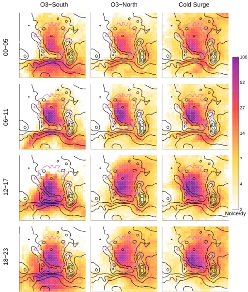
00−05

06−11

12−17

18−23

O3−South O3−North Cold Surge

2 4 7 14 27 52 100 No/ce/dy

Fig. 8. Column “concentration fields” by time of day and by episode for CO tracers for the small domain. Values correspond to the count

of particles vertically integrated for each grid cell over the entire campaign normalised by the number of days in each episode (No/ce/dy = Number per cell per day). Non-dimensionally, this is similar to a plume column concentration diagram showing the urban impacts. Black terrain contour lines shown every 500 m, political boundary of the MCMA in pink.

histogram of recirculation fractions by episode type is also shown in Fig. 7. These are regular histograms where the bars have been replaced by lines so that the histograms from the 3 episodes could be overlayed. The median recirculation frac-tion is 42% for O3-South days, 12% for O3-North and 27% for Cold Surge.

Figure 8 shows the sum of column concentration fields on the basin grid by episode type and by time of day. For O3-South days, the dominant feature is transport to the O3-South for all times of the day. Outflow from the basin takes place along the entire southern rim of the basin. In the morning, there is more flow through the Chalco passage in the southeast, but later in the day the outflow is greater to the southwest near the Ajusco mountain (at the Tres Marias pass). High

concen-trations of polluted air exist south of the basin rim above the mountain slopes as basin air meets up-valley flow from the south. This is strong enough in the evening to push part of the urban plume over Toluca to the west and Puebla to the east. Some transport to the north can be seen, with northeast impacts from afternoon releases and northwest impacts from the night-time releases. The impacts to the north are minimal during the day but increase at night in the north and northeast of the city.

For O3-North days, the dominant outflux from the urban area can be seen to the northeast and southeast. In the early morning, there are high concentrations to the south of the basin in the Cuautla valley and to the east over Puebla. As mixing heights rise during the day, these impacts are reduced.

Fig. 9. Basin outflow “residence times” for CO tracers by height and by episode type in units of number per cell per day. Cells are between

35 and 40 km rings around MCMA, and are vertically resolved from the surface to 2000 m a.g.l. in 250 m increments. The MCMA is inside the cylinder, view looking towards the Chalco passage in the southeast with north at the bottom.

00−05

06−11

12−17

18−23

O3−South O3−North Cold Surge

1 2 4 8 17 34 70 No/ce/dy

Fig. 10. Column “residence time” fields by time of day and by episode for backward MCMA trajectories for the small domain (No/ce/dy =

Number per cell per day). This shows the path taken for particles arriving in the MCMA at each particular time range. Black terrain contour lines shown every 500 m, political boundary of the MCMA in pink.

0 24 48 72 96 120 144 0 10 20 30 40 50 Histogram (%)

Time before leaving the basin (Hr) Residence Times O3−South O3−North Cold Surge 0 10 20 30 40 50 60 70 80 90 100 0 10 20 30 40 50 Histogram (%) Recirculation Fraction (%) Recirculation Fractions O3−South O3−North Cold Surge

Fig. 11. Residence time and recirculation fractions for the regional domain bounded by the Gulf and Pacific coasts truncated 600 km to the

North and 800 km to the East. See Fig. 7 for explanation of plots.

There are late morning impacts through the Chalco passage and to the south of the basin. These are replaced with north-east impacts as the afternoon progresses. By night, concen-trations are high on the whole eastern edge of the domain suggesting impacts from flow going on both sides of the vol-canoes.

For Cold Surge days there is a clearer channelling of night-time flows through the Chalco passage, although there are also impacts to the northeast and looping around the volca-noes to Puebla. As the day progresses, the impacts are more clearly to the south in areas of low terrain elevation, with lit-tle flow over the basin rim and lower concentrations over the volcanoes. By night-time, there is a northward component affecting the northeast of the city and the regions to the east of the basin.

Figure 9 shows residence time plots resolved in the ver-tical for a circular area around the basin. Hourly particle path positions were counted in area between 35 and 45 km from a point near the airport (UTM coordinates: 490 E, 2150 N km, zone 14) with a vertical resolution of 250 m up to 2000 m a.g.l. As before, these are summed over all time periods by episode, and is a non-dimensional representation of the time spent by the particles in the ring surrounding the city. On O3-South days, the outflow can be clearly seen over the basin rim in the south. The highest residence times are above the surface, between 250 and 1000 m a.g.l. On O3-North days, the component of outflow towards the south is much weaker as well as being a little higher and over to the southeast. The main outflow can be clearly seen to the north and northeast. The highest concentrations are at the surface but for the northeast the plume maximum is in the 500 to 750 m a.g.l. range. On Cold Surge days the outflow is to the south. In contrast with O3-South days however, the bulk of

the flow is near the surface in the Chalco pass to the south-east. Reduced vertical mixing leads to higher residence times close to the surface for all exit directions.

4.2 Basin inflow

Residence time fields for backward trajectories from the ur-ban area are shown in Fig. 10 by episode and by time of day. These show where the air mass over the city originated on the local scale. For O3-South days, the night time flow is a combination of flow from the Mexican plateau in the north and through the Chalco pass in the southeast. The Mexi-can plateau flow increases during the day and dominates the afternoon inflow before the gap flow resumes in the early evening. For O3-North days, the situation is similar although the inflow comes much more strongly from the west. This increases as the day progresses and dominates the afternoon flow with air from Toluca coming over the mountain pass in the west of the basin. As the evening progresses, the inflows come around the Ajusco mountain in the southwest of the basin. Cold surge days have a strong inflow from the north for all time periods. During the day there is a slightly in-creasing component from the northeast reverting to air com-ing from the northwest at night.

4.3 Region outflow

On the regional scale, the residence time of the urban plume over land is shown in Fig. 11 along with the recirculation fractions. The median residence times are 4.7 days for O3-South, 2.5 days for O3-North and 2 days for Cold Surge. More than one quarter of trajectories from O3-South days were still over land at the end of the 6 day simulation period. Recirculation fractions show a median of 37% for O3-South

2330 B. de Foy et al.: Mexico City basin ventilation and urban plume 0 24 48 72 96 120 144 0 10 20 30 40 Histogram (%)

Time before leaving the basin (Hr) O3−South O3−North Cold Surge 0 10 20 30 40 50 60 70 80 90 100 0 10 20 30 40 Histogram (%) Recirculation Fraction (%) O3−South O3−North Cold Surge

Fig. 11. Residence time and recirculation fractions for the regional domain bounded by the Gulf and Pacific

coasts truncated 600 km to the North and 800 km to the East. See Fig. 7 for explanation of plots.

O3−South O3−North Cold Surge

10 26 67 173 448 1159 3000 No/ce/dy

Fig. 12. Column “concentration fields” for forward trajectories for the regional domain by episode type, cf.

Fig. 8.

Fig. 13. Regional outflow “residence times” for CO tracers by height and by episode type, cf. Fig. 9. Particle

counts in 300 to 400 km ring around MCMA, vertical grid from surface to 8000 magl in 250 m increments. Mountains surrounding the basin can be seen in the middle of the cylinder with the Pacific Ocean on the bottom, the Gulf of Mexico on the top of the figure and North to the left. Acapulco is along the piece of coast hidden by the cylinder and Veracruz along the coast hidden by the volcanoes inside the cylinder.

26

Fig. 12. Column “concentration fields” for forward trajectories for the regional domain by episode type, cf. Fig. 8.

days compared with 29% and 28% for O3-North and Cold Surge respectively. These are particles that leave the domain either over the Gulf or over the Pacific before being blown back to land.

The regional impact does not vary substantially by time of day and is shown by episode type in Fig. 12 on the medium grid with 36 km spacing. On O3-South days, the plume leaves the basin mainly to the south as shown above. Af-ter that it fans out and impacts both the Pacific coast to the south and the Gulf coast to the east. The column concen-tration plots show some looping around the Pico de Orizaba volcano due east, with northward transport along the flanks of the Sierra Madre Oriental.

On O3-North days, the north-eastward outflow from the basin continues in the same direction, moving over the Sierra Madre Oriental and onto the Gulf of Mexico. The outflow to the south and southwest is limited to the area adjacent to the basin as further away the plume is blown back to the east and northeast.

On Cold Surge days, the column integrated spatial im-pact is similar to O3-North days with outflow to the north-east. The main difference is that the plume follows the ter-rain much more closely as it is channelled through mountain passes and depressions. On the basin scale, the outflow was mainly to the south through the Chalco passage. This can be seen on the regional plot but lasts for less than 100 km as the flow is turned to the northeast. The outflow is concentrated beyond Pachuca in the valleys descending the Sierra Madre Oriental. After this, it fans out along the coast impacting ar-eas both to the north and south.

Figure 13 shows the exit direction on the regional scale resolved vertically. Particle paths were gridded radially be-tween 300 and 400 km from the MCMA. In the vertical, the resolution is 250 m and extends to 8000 m a.g.l. For O3-South days, this shows outflow towards the south in the range of 1500 to 2500 m a.g.l. and towards the southwest around 3000 m a.g.l. The component of northward flow can be seen in the lower levels along the Gulf Coast and out over the Gulf. For O3-North days, two dominant outflow areas can be seen. To the north near the Sierra Madre Oriental there is a low level outflow around 500 to 1000 m a.g.l. To the east, the

peak outflow is in the range of 3000 to 4000 m a.g.l., but the outflow is widely spread out both vertically and for the entire northeast quadrant. Cold Surge days have the most outflow in the lower levels along the flank of the Sierra Madre Orien-tal. There is no outflow for the whole western side and some outflow over the Gulf at higher elevations.

4.4 Region inflow

Residence time fields for backward trajectories from the ur-ban area are shown in Fig. 14 fro the large domain separated by episode. For O3-South days, air from the Pacific ocean flows along the coast and enters the basin either from the northwest over the Mexican plateau or from the southwest through the valley of the Rio Balsas. There is some flow from the southern Pacific that is taken up in the northward valley flows. Impact from the Gulf is limited to an influx from the southeast that moves northwards along the coast.

For O3-North days, the inflow is much more focussed on the valley of the Rio Balsas drawing air from the Pacific coast both to the north and south of the river mouth. As the flow ap-proaches the basin, it enters from both the southern and west-ern rim. There is some impact from the Mexican plateau and also from the Gulf coast entering the basin from the north.

Because of the greater internal variation of Cold Surge days, the inflow can be seen to come from many direc-tions. One noticeable feature are the sharper gradients fol-lowing the topography, as the lower mixing heights lead to increased terrain channelling. The main inflow direction is from the north with Gulf air moving over Pachuca into the basin. There is additional inflow from the Sierra Madre Ori-ental south of the Pico de Orizaba meeting Pacific inflow and entering the basin from the south.

5 Discussion

The results section presented aggregate behaviour of the plume by episode type, showing distinct ventilation patterns and residence times for each type. This section will focus on three specific days to analyse in greater detail the pro-cesses causing the observed results. Following de Foy et al.

Fig. 13. Regional outflow “residence times” for CO tracers by height and by episode type, cf. Fig. 9, in units of number per cell per day.

Cells are between 300 and 400 km rings around MCMA, and are vertically resolved from the surface to 8000 m a.g.l. in 250 m increments. Mountains surrounding the basin can be seen in the middle of the cylinder with the Pacific Ocean on the bottom, the Gulf of Mexico on the top of the figure and North to the left. Acapulco is along the piece of coast hidden by the cylinder and Veracruz along the coast hidden by the volcanoes inside the cylinder.

O3−South O3−North Cold Surge

50 82 136 224 368 607 1000 No/ce/dy

Fig. 14.Column “residence time” field by episode for backward MCMA trajectories for the large domain, cf.

Fig. 10.

Fig. 15. Particle clouds at 18:00 CDT for the three cases described in the text on the regional scale (top) and

the basin scale (bottom). Particles are coloured according to height above ground level. Top stars correspond to MCMA (centre) and Veracruz (left), bottom stars correspond to CENICA, T1 and T2. Black terrain contour lines shown every 500 m, political boundary of the MCMA in pink.

Fig. 14. Column “residence time” field by episode for backward MCMA trajectories for the large domain, cf. Fig. 10.

(2005b), 15 April was chosen for the O3-South category, 23 April for O3-North and 8 April for Cold Surge. Figure 15 shows the particle cloud (snapshot of current particles for all prior releases) of the urban plume at 18:00 for each day at both the regional and basin scale. North-south cross-sections of the basin are shown in Fig. 16. Finally, particle paths (hourly positions of a single release for the entire simulation period) from specific releases around the basin are shown in Fig. 17 to help elucidate the flow patterns entering the basin. 15 April shows the clockwise transport aloft by an anti-cyclone over western Mexico characteristic of O3-South episodes. At lower levels however, the plume is taken into the northward surface flow of the Gulf of Mexico along the edge of the Sierra Madre Oriental. This section of the plume comes from the night time surface flow blown northward by the low level jet. There is a return flow visible on the regional scale as the convergence line between the Pacific ocean breeze and the Gulf breeze moves south-eastward. On the basin scale, the cross-section looking west shows clearly the vertical dispersion of the urban plume to 4000 m a.g.l. Close inspection of the fresh particles on the southern slope show that there is some up-slope flow but that the majority of the transport is due to vertical mixing above the city. In this case, the increased mixing heights over the urban area

dom-inate the up-slope drafts. Once the plume is aloft, it is trans-ported southwards where it meets the cooler ocean air mov-ing up-valley. This leads to an accumulation band at around 4000 m a.s.l. with little MCMA impacts at the surface. The flow is relatively stationary at this point and flows back into the basin when the northward jet forms in the Chalco pas-sage. The (relatively) aged particles stay mainly on the east-ern edge of the basin before being vented out again by ver-tical mixing. Looking at the particle releases from points around the basin confirms this picture. The releases to the north of the basin are convected into the basin and over the rim to the Cuautla valley. The release in the Chalco passage leads to a sharply defined influx on the eastern edge of the basin before being blown eastward through a combination of convection and vertical mixing.

23 April has a strong north-eastward outflow typical of O3-North days. Vigorous vertical mixing takes place dilut-ing the plume more than 4000 m a.g.l. In addition, for this particular case, a strong convective cell developed in the af-ternoon (de Foy et al., 2005b) explaining the transport above the top of the mixing layer. Low particle densities exist in the basin at 18:00 as the plume is swept away by a strong north-eastward flow over the western and southern edges of the basin. On the regional scale, there is a vertical separation

2332 B. de Foy et al.: Mexico City basin ventilation and urban plume 50 82 136 224 368 607 1000 No/ce/dy

Fig. 14. Column “residence time” field by episode for backward MCMA trajectories for the large domain, cf. Fig. 10.

Fig. 15. Particle clouds at 18:00 CDT for the three cases described in the text on the regional scale (top) and the basin scale (bottom). Particles are coloured according to height above ground level. Top stars correspond to MCMA (centre) and Veracruz (left), bottom stars correspond to CENICA, T1 and T2. Black terrain contour lines shown every 500 m, political boundary of the MCMA in pink.

27

Fig. 15. Particle clouds at 18:00 CDT for the three cases described in the text on the regional scale (top) and the basin scale (bottom).

Particles are coloured according to height above ground level. Top stars correspond to MCMA (centre) and Veracruz (left), bottom stars correspond to CENICA, T1 and T2. Black terrain contour lines shown every 500 m, political boundary of the MCMA in pink.

between the flow aloft which is taken east and even southeast towards the Gulf and the surface flow which is much slower and leads to more concentrated impacts moving north along the Gulf coast. In contrast with 15 April, this flow does not impact the Mexican plateau as the regional convergence line stays close to the edge of the Sierra Madre Oriental. Parti-cle paths from the release to the north of the basin reveal the strong eastward component of the flow with little impact on the MCMA. The release in the Chalco passage does show the jet flow very clearly however and impacts much more of the urban area as it moves north-westward before being taken up in the regional eastward movement. The release near Cuautla is also influenced by the eastward flow preventing it from en-tering the basin at Chalco and impacting Puebla instead.

8 April was the day of highest rain from the field campaign and the central day of a Cold Surge episode. As expected, the surface transport is to the south with strong channelling through the Chalco passage. On the basin scale, the reduced vertical mixing leads to particles accumulating in the basin and held back by the surrounding mountains. The outflow through Chalco leads to surface transport down the Cuautla valley. This time, there is no up-coming valley flow to coun-teract the jet. There are older particles that experienced in-creased vertical transport earlier in the day when the mixing height was higher. These are transported both southward and eastward. On the regional scale, these particles are caught in

the westerlies and blown eastward over the Gulf. This leads to a plume split in two with each half travelling in opposite directions. Particles released near Pachuca show the strong inflow into the basin. This has a westward component as the flow from the Gulf blows perpendicular to the mountain axis. The flow in the Chalco passage fans out to the south impact-ing the whole Cuautla valley.

6 Conclusions

The FLEXPART trajectory model was used with MM5 sim-ulated wind fields to analyse the air flow in the Mexico City basin. Mixing heights simulated by MM5 were shown to be in good agreement with those obtained from radiosonde ob-servations, giving confidence in the model representation of vertical diffusion. Model simulated virtual balloon trajecto-ries were compared against a rich dataset of pilot balloon trajectories consisting of 409 releases from 3 sites during the whole time of the campaign. There is a large variabil-ity between the virtual balloon trajectories due to the weak and variable winds. This suggests that the bounds on the expected accuracy of a point-to-point comparison are rather large. 50% of trajectories had relative errors smaller than 50%, suggesting that the model is able to reproduce the flow features in the basin. Further comparisons were made be-tween model trajectories and radiosonde paths with similar

Fig. 16.Particle cloud cross-section at 18:00 CDT for the three cases described in the text. Vertical slice along line AB (Fig. 2), showing particles to the west (top) and to the east (bottom). Particles coloured by age.

Pass South NE NW

Release

15−Apr−2003 18:00 23−Apr−2003 18:00 08−Apr−2003 18:00

Fig. 17.Particle paths from four releases on the basin periphery at 18:00 CDT for the three cases described in the text. Pass (red) is in the Chalco passage, South (yellow) in the Cuautla valley, NE (blue) near Pachuca and NW (green) to the north-west.

Fig. 16. Particle cloud cross-section at 18:00 CDT for the three cases described in the text. Vertical slice along line AB (Fig. 2), showing

particles to the west (top) and to the east (bottom). Particles coloured by age.

Fig. 16.Particle cloud cross-section at 18:00 CDT for the three cases described in the text. Vertical slice along line AB (Fig. 2), showing particles to the west (top) and to the east (bottom). Particles coloured by age.

Pass South NE NW

Release

15−Apr−2003 18:00 23−Apr−2003 18:00 08−Apr−2003 18:00

Fig. 17. Particle paths from four releases on the basin periphery at 18:00 CDT for the three cases described in the text. Pass (red) is in the Chalco passage, South (yellow) in the Cuautla valley, NE (blue) near Pachuca and NW (green) to the north-west.

28

Fig. 17. Particle paths from four releases on the basin periphery at 18:00 CDT for the three cases described in the text. Pass (red) is in the

Chalco passage, South (yellow) in the Cuautla valley, NE (blue) near Pachuca and NW (green) to the northwest.

accuracy levels. As these are more widely available, albeit with reduced spatial and temporal coverage, they could serve for model comparisons and evaluation in a greater number of cases. The variability in the trajectories could also serve as an estimate of the expected variability in sounding data for model validation.

Forward trajectories were simulated corresponding to ur-ban primary emissions. Backward trajectories traced the ori-gin of the air people breathe in the basin. Venting of the

basin was found to be very rapid, especially for 2 of the 3 episode types studied: O3-North and Cold Surge. Resi-dence times below 7 h for 50% of particles corroborate find-ings from previous studies. On the regional scale, the trans-port is equally rapid, with 50% of particles remaining over land for less than 2 to 2.5 days. There is however a sig-nificant amount of recirculation and longer residence times for O3-South episodes. Peak ozone values during the cam-paign occurred on all three episode types suggesting that

O3-South

O3-North

Cold Surge

Fig. 18. Circulation Model for the Mexico City basin for O3-South, O3-North and Cold Surge episode types. Arrows coloured by time of day: early morning (0-5) in blue, morning (6-11) in red, afternoon (12-17) in brown and evening (18-23) in yellow. Plateau winds on O3-South days combine with vigorous mixing to transport the urban plume southwards of the mountains. A low level jet forms in the Chalco passage causing a convergence line in the south of the city. Strong westerly flow on O3-North days first enters the basin from the north-west but then comes over the south and west rims of the basin during the day. The combination with the low level jet forms a north-south convergence zone and exhaust of the basin to the north-east. On Cold Surge days strong northerly winds blow into the basin. Low mixing heights lead to pollutant accumulation in the city and channel flow through the Chalco passage.

Fig. 18. Circulation Model for the Mexico City basin for O3-South, O3-North and Cold Surge episode types. Arrows coloured by time

of day: early morning (0–5) in blue, morning (6–11) in red, afternoon (12–17) in brown and evening (18–23) in yellow. Plateau winds on O3-South days combine with vigorous mixing to transport the urban plume southwards of the mountains. A low level jet forms in the Chalco passage causing a convergence line in the south of the city. Strong westerly flow on O3-North days first enters the basin from the northwest but then comes over the south and west rims of the basin during the day. The combination with the low level jet forms a north-south convergence zone and exhaust of the basin to the northeast. On Cold Surge days strong northerly winds blow into the basin. Low mixing heights lead to pollutant accumulation in the city and channel flow through the Chalco passage.

multi-day carry-over may contribute to greater spatial ex-tent of the ozone peak but not to the maximum daily value (de Foy et al., 2005a). In this respect, Mexico City is more comparable to Houston and Athens where sea-breeze flows lead to same-day convergence of emissions over the urban area rather than Los Angeles where a polluted reservoir is formed. The mountain basin acts as an “air pump” pulsing the urban plume aloft after which it is carried away by the synoptic flow. The vigorous vertical mixing dominates both the slope flow and the wind convergence updrafts, leading to a well-mixed vertical plume over the urban area. On the regional scale, for this time of year, the main directions of outflow of the basin are east and northeast with some limited transport to the Pacific ocean on certain days.

The circulation model proposed in de Foy et al. (2005a) is revised in Fig. 18 in the light of the wind convergence pat-terns of de Foy et al. (2005b) and the current particle tra-jectories. These effects, and especially their vertical resolu-tion, enhance the previous model which was based on sur-face wind measurements. For O3-South days, the plateau-to-basin winds are the main influx into the plateau-to-basin coming from the north in the afternoon and from the northwest the rest of the time. The low level jet through the Chalco passage forms in the evening and continues throughout the night. The plume is mixed vertically and transported out of the basin southwards above the mountains. For O3-North days, the in-flux is in the north of the basin, but coming from the west. Rather than being a plateau flow, it is actually an up-valley flow through the Rio Balsas valley, up to Toluca and around the mountains. As the day progresses, the westerly flow strengthens and comes over the basin rim on both sides of the Ajusco mountain. The low level jet in the Chalco pas-sage is now an extension of this flow rather than a separate feature. Plume exhaust takes place along the axis of the

con-vergence line towards the northeast. For Cold Surge days, the inflow is from the north. Low mixing heights lead to an accu-mulation in the middle of the basin with outflow southward through the Chalco passage. Mountain blocking of the flow is particularly noticeable at night with flow on both sides of the volcanoes in the southeast.

While a limited number of cases were presented in this paper, trajectories were generated for the whole campaign forming a database for the analysis of MCMA-2003 wind transport, which is currently accessible from http://mce2.org/ as part of the MCMA-2003 and MCMA-2006 field cam-paigns. It is hoped that this may help in interpreting ob-servations from the field campaign and in planning for the up-coming MILAGRO campaign (Megacity Initiative: Lo-cal and Global Research Observations, http://www.joss.ucar. edu/milagro/). The analysis of flow patterns and residence times will also be able to assist in developing abatement strategies and provide policy guidance for reducing the ad-verse health impacts on the public.

Acknowledgements. The authors wish to thank the Pilot Balloon

Team at the Universidad Aut´onoma Metropolitana, Mexico, for the database of balloon trajectories. Radiosonde observations were pro-vided by the Mexican National Meteorological Service with support from Pemex-Refinaci´on to the Instituto Mexicano del Petr´oleo for additional soundings at 06:00 and 18:00 UTC, operated by the Cen-tro de Ciencias de la Atm´osfera, Universidad Nacional Aut´onoma de M´exico.

MM5 is made publicly available and supported by the Mesoscale and Microscale Meteorology division at the National Center for At-mospheric Research for which the authors are very grateful. The authors thank A. Stohl for making FLEXPART available and for valuable discussions, G. Wotawa for developing the MM5 version and two anonymous referees for their reviews.

The financial support from the US National Science Foundation (Award ATM-0511803) and the US Department of Energy (Award DE-FG02-05ER63980) for this work is gratefully acknowledged. Edited by: C. E. Kolb

References

Ashbaugh, L. L., Malm, W. C., and Sadeh, W. Z.: A residence time probability analysis of sulfur concentrations at Grand Canyon National Park, Atmos. Environ., 19, 1263–1270, 1985.

Banta, R. M., Seniff, C. J., Nielsen-Gammon, J., Darby, L. S., Ry-erson, T. B., Alvarez, R. J., Sandberg, S. R., Williams, E. J., and Trainer, M.: A bad air day in Houston, Bull. Amer. Met. Soc., 86, 657–669, 2005.

Baumann, K. and Stohl, A.: Validation of a long-range trajectory model using gas balloon tracks from the Gordon Bennett Cup 95, J. Appl. Meteorol., 36, 711–720, 1997.

Bossert, J. E.: An investigation of flow regimes affecting the Mex-ico City region, J. Appl. Meteorol., 36, 119–140, 1997. Brulfert, G., Chemel, C., Chaxel, E., and Chollet, J. P.: Modelling

photochemistry in alpine valleys, Atmos. Chem. Phys., 5, 2341– 2355, 2005, http://www.atmos-chem-phys.net/5/2341/2005/. de Foy, B., Caetano, E., Maga˜na, V., Zit´acuaro, A., C´ardenas, B.,

Retama, A., Ramos, R., Molina, L. T., and Molina, M. J.: Mexico City basin wind circulation during the MCMA-2003 field cam-paign, Atmos. Chem. Phys., 5, 2267–2288, 2005a.

de Foy, B., Clappier, A., Molina, L. T., and Molina, M. J.: Dis-tinct wind convergence patterns in the Mexico City basin due to the interaction of the gap winds with the synoptic flow, Atmos. Chem. Phys., 6, 1 249–1 265, 2005b.

de Foy, B., Molina, L. T., and Molina, M. J.: Satellite-derived land surface parameters for mesoscale modelling of the Mexico City basin, Atmos. Chem. Phys., 5, 9861–9906, 2005c.

Fast, J. D. and Zhong, S. Y.: Meteorological factors associated with inhomogeneous ozone concentrations within the Mexico City basin, J. Geophys. Res.-Atmos., 103, 18 927–18 946, 1998. Fast, J. D., Doran, J. C., Shaw, W. J., Coulter, R. L., and Martin,

T. J.: The evolution of the boundary layer and its effect on air chemistry in the Phoenix area, J. Geophys. Res.-Atmos., 105, 22 833–22 848, 2000.

Grell, G. A., Dudhia, J., and Stauffer, D. R.: A Description of the Fifth-Generation Penn State/NCAR Mesoscale Model (MM5), Tech. Rep. NCAR/TN-398+STR, NCAR, 1995.

Grossi, P., Thunis, P., Martilli, A., and Clappier, A.: Effect of sea breeze on air pollution in the Greater Athens Area. Part II: Anal-ysis of different emission scenarios, J. Appl. Meteorol., 39, 563– 575, 2000.

Henne, S., Furger, M., Nyeki, S., Steinbacher, M., Neininger, B., de Wekker, S. F. J., Dommen, J., Spichtinger, N., Stohl, A., and Prevot, A. S. H.: Quantification of topographic venting of bound-ary layer air to the free troposphere, Atmos. Chem. Phys., 4, 497– 509, 2004, http://www.atmos-chem-phys.net/4/497/2004/.

Hong, S. Y. and Pan, H. L.: Nonlocal boundary layer vertical dif-fusion in a Medium-Range Forecast Model, Mon. Weather Rev., 124, 2322–2339, 1996.

Jazcilevich, A. D., Garc´ıa, A. R., and Ruiz-Suarez, L. G.: A study of air flow patterns affecting pollutant concentrations in the Central Region of Mexico, Atmos. Environ., 37, 183–193, 2003. Jazcilevich, A. D., Garcia, A. R., and Caetano, E.: Locally induced

surface air confluence by complex terrain and its effects on air pollution in the valley of Mexico, Atmos. Environ., 39, 5481– 5489, 2005.

Kalthoff, N., Kottmeier, C., Thurauf, J., Corsmeier, U., Said, F., Frejafon, E., and Perros, P. E.: Mesoscale circulation systems and ozone concentrations during ESCOMPTE: a case study from IOP 2b, Atmos. Res., 74, 355–380, 2005.

Lehning, M., Richner, H., Kok, G. L., and Neininger, B.: Verti-cal exchange and regional budgets of air pollutants over densely populated areas, Atmos. Environ., 32, 1353–1363, 1998. Lu, R. and Turco, R. P.: Air pollutant transport in a coastal

en-vironment. 2. 3-dimensional simulations over los-angeles basin, Atmos. Environ., 29, 1499–1518, 1995.

Menut, L., Vautard, R., Flamant, C., Abonnel, C., Beekmann, M., Chazette, P., Flamant, P. H., Gombert, D., Guedalia, D., Kley, D., Lefebvre, M. P., Lossec, B., Martin, D., Megie, G., Per-ros, P., Sicard, M., and Toupance, G.: Measurements and mod-elling of atmospheric pollution over the Paris area: an overview of the ESQUIF Project, Ann. Geophys., 18, 1467–1481, 2000, http://www.ann-geophys.net/18/1467/2000/.

Schmitz, R.: Modelling of air pollution dispersion in Santiago de Chile, Atmos. Environ., 39, 2035–2047, 2005.

Stohl, A.: Computation, accuracy and applications of trajectories – A review and bibliography, Atmos. Environ., 32, 947–966, 1998. Stohl, A. and Thomson, D. J.: A density correction for Lagrangian particle dispersion models, Boundary-Layer Meteorol., 90, 155– 167, 1999.

Stohl, A., Hittenberger, M., and Wotawa, G.: Validation of the Lagrangian particle dispersion model FLEXPART against large-scale tracer experiment data, Atmos. Environ., 32, 4245–4264, 1998.

Stohl, A., Forster, C., Frank, A., Seibert, P., and Wotawa, G.: Tech-nical note: The Lagrangian particle dispersion model FLEX-PART version 6.2, Atmos. Chem. Phys., 5, 2461–2474, 2005, http://www.atmos-chem-phys.net/5/2461/2005/.

West, J. J., Zavala, M. A., Molina, L. T., Molina, M. J., San Mar-tini, F., McRae, G. J., Sosa-Iglesias, G., and Arriaga-Colina, J. L.: Modeling ozone photochemistry and evaluation of hydro-carbon emissions in the Mexico City metropolitan area, J. Geo-phys. Res.-Atmos., 109, doi:10.1029/2004JD004614, 2004. Williams, M. D., Brown, M. J., Cruz, X., Sosa, G., and Streit, G.:

Development and testing of meteorology and air dispersion mod-els for Mexico City, Atmos. Environ., 29, 2929, 1995.