HAL Id: cea-02266323
https://hal-cea.archives-ouvertes.fr/cea-02266323
Submitted on 13 Aug 2019
HAL is a multi-disciplinary open access
archive for the deposit and dissemination of
sci-entific research documents, whether they are
pub-lished or not. The documents may come from
teaching and research institutions in France or
abroad, or from public or private research centers.
L’archive ouverte pluridisciplinaire HAL, est
destinée au dépôt et à la diffusion de documents
scientifiques de niveau recherche, publiés ou non,
émanant des établissements d’enseignement et de
recherche français ou étrangers, des laboratoires
publics ou privés.
The Most Massive galaxy Clusters (M2C) across cosmic
time: link between radial total mass distribution and
dynamical state
I. Bartalucci, M. Arnaud, G. W. Pratt, J. Démoclès, L. Lovisari
To cite this version:
I. Bartalucci, M. Arnaud, G. W. Pratt, J. Démoclès, L. Lovisari. The Most Massive galaxy Clusters
(M2C) across cosmic time: link between radial total mass distribution and dynamical state. Astronomy
and Astrophysics - A&A, EDP Sciences, 2019, 628, pp.A86. �10.1051/0004-6361/201935984�.
�cea-02266323�
https://doi.org/10.1051/0004-6361/201935984 c I. Bartalucci et al. 2019
Astronomy
&
Astrophysics
The Most Massive galaxy Clusters (M2C) across cosmic time: link
between radial total mass distribution and dynamical state
I. Bartalucci
1, M. Arnaud
1, G. W. Pratt
1, J. Démoclès
1, and L. Lovisari
21 AIM, CEA, CNRS, Université Paris-Saclay, Université Paris Diderot, Sorbonne Paris Cité, 91191 Gif-sur-Yvette, France
e-mail: iacopo.bartalucci@cea.fr
2 Center for Astrophysics| Harvard & Smithsonian, 60 Garden Street, Cambridge, MA 02138, USA
Received 29 May 2019/ Accepted 3 July 2019
ABSTRACT
We study the dynamical state and the integrated total mass profiles of 75 massive (M500 > 5 × 10¹⁴M )
Sunyaev–Zeldovich(SZ)-selected clusters at 0.08 < z < 1.1. The sample is built from the Planck catalogue, with the addition of four SPT clusters at z > 0.9. Using XMM-Newton imaging observations, we characterise the dynamical state with the centroid shift hwi, the concentration CSB, and their combination, M, which simultaneously probes the core and the large-scale gas morphology. Using spatially resolved
spectroscopy and assuming hydrostatic equilibrium, we derive the total integrated mass profiles. The mass profile shape is quantified by the sparsity, that is the ratio of M500to M2500, the masses at density contrasts of 500 and 2500, respectively. We study the correlations
between the various parameters and their dependence on redshift. We confirm that SZ-selected samples, thought to most accurately reflect the underlying cluster population, are dominated by disturbed and non-cool core objects at all redshifts. There is no significant evolution or mass dependence of either the cool core fraction or the centroid shift parameter. The M parameter evolves slightly with z, having a correlation coefficient of ρ = −0.2 ± 0.1 and a null hypothesis p-value of 0.01. In the high-mass regime considered here, the sparsity evolves minimally with redshift, increasing by 10% between z < 0.2 and z > 0.55, an effect that is significant at less than 2σ. In contrast, the dependence of the sparsity on dynamical state is much stronger, increasing by a factor of ∼60% from the one third most relaxed to the one third most disturbed objects, an effect that is significant at more than 3σ. This is the first observational evidence that the shape of the integrated total mass profile in massive clusters is principally governed by the dynamical state and is only mildly dependent on redshift. We discuss the consequences for the comparison between observations and theoretical predictions.
Key words. dark matter – galaxies: clusters: intracluster medium – X-rays: galaxies: clusters
1. Introduction
The shape of the dark matter profile in galaxy clusters is a sen-sitive test of the nature of dark matter and of the theoretical scenario of structure formation. In the standard framework, cos-mological structures form hierarchically from initial density fluctuations that grow under the influence of gravity. In aΛ cold dark matter (ΛCDM) Universe, the dark matter (DM) collapse is scale-free and one expects objects to form with similar inter-nal structure. The DM shape is expected to depend on the halo assembly history, which is a function of the redshift, the total mass, and the underlying cosmology (e.g. Dolag et al. 2004;
Kravtsov & Borgani 2012). A certain scatter of the shape and break of strict self-similarity are expected, reflecting the detailed formation history of each halo.
Clusters of galaxies are ideal targets to test the above sce-nario: the dark matter is the dominant component by far except in the very centre. Furthermore, complementary techniques can measure the total mass density profile, for example, galaxy velocities; strong gravitational lensing in the centre and weak lensing at large scale; X-ray estimates using the intra-cluster medium (ICM) density and temperature profiles and the hydro-static equilibrium (HE) equation (see Pratt et al. 2019, for a review).
Numerical simulations indeed predict that the cold dark mat-ter density profiles of virialised objects follows a ‘universal’ form. Well-known parametric models for the DM density pro-files include those proposed byNavarro et al. (1997; hereafter
NFW) and the Einasto profile (Einasto 1965), which is currently considered to be a more accurate description of the profiles in state-of-the-art simulations (Navarro et al. 2004;Wu et al. 2013). A fundamental parameter of these parametric models is their concentration, which in general terms describes the relative dis-tribution in the core as compared to the outer region (Klypin et al. 2016). The concentration is characterised in the NFW and Einasto1 models by the ratio c ≡ r
−2/R∆2, where r−2 is the
radius at which the logarithmic density slope is equal to −2. The relation between the concentration and the total mass (here-after c−M) has been very widely used as an indicator of the dark matter profile shape in cosmological simulations (e.g. Diemer & Kravtsov 2015, and references therein). However, it has been shown that the c−M relation of the most relaxed haloes is di ffer-ent to that derived for the full population (e.g.Neto et al. 2007;
Bhattacharya et al. 2013). In fact, the capability of these para-metric models to reproduce the DM profile (i.e. the goodness of the fit) depends on the dynamical state of the halo and on the formation time (Jing 2000;Wu et al. 2013, for the NFW case). Results on the dependence of the DM profile shape on mass and redshift based on c−M relations may thus be ambiguous, and depend on the sample selection (Klypin et al. 2016;Balmès et al. 2014). For this reason, recent works based on simulations have
1 In this model, the actual shape also depends on a second parameter. 2 R
∆is defined as the radius enclosing∆ times the critical matter
den-sity at the cluster redshift. M∆is the corresponding mass.
Open Access article,published by EDP Sciences, under the terms of the Creative Commons Attribution License (http://creativecommons.org/licenses/by/4.0),
often focused on relaxed haloes (e.g. Dutton & Macciò 2014;
Ludlow et al. 2014;Correa et al. 2015).
However, a rigorous comparison with cluster observations cannot be made, as there is a continuous distribution of dynam-ical states, and the definition of what is a relaxed object is therefore somewhat arbitrary. Moreover, in the absence of fully realistic simulations including the complex baryonic physics, it is nearly impossible to define common criteria that quantify the dynamical state in a consistent manner, both in simulations and observations. Ideally we would compare the full cluster popula-tion from numerical simulapopula-tions to observed samples chosen to reflect as closely as possible the true underlying population. The advent of Sunyaev–Zeldovich (SZ)-selected cluster catalogues offers a unique opportunity to build such observational samples. Surveys such as those from the Atacama Cosmology Telescope (ACT; Marriage et al. 2011), the South Pole Telescope (SPT;
Reichardt et al. 2013;Bleem et al. 2015), and the Planck Sur-veyor (Planck Collaboration VIII 2011; Planck Collaboration XXIX 2014;Planck Collaboration XXVII 2016) have provided SZ-selected cluster samples up to z ∼ 1.5. The magnitude of the SZ effect being closely linked to the underlying mass with small scatter (da Silva et al. 2004), these are thought to be as near as possible to being mass selected, and as such unbiased.
The observational study of the DM profile shape using such samples requires investigation of the dependence on fundamen-tal cluster quantities such as mass, dynamical state, and red-shift. X-ray observations are an excellent tool with which to undertake such studies – the ICM morphology can be used to infer the dynamical state, while the total mass profile can be derived by applying the hydrostatic equilibrium (HE) equation to spatially resolved density and temperature profiles. While this method yields the highest statistical precision on individual pro-files over a wide radial range and up to high z (Amodeo et al. 2016;Bartalucci et al. 2018), it has the drawback of a systematic uncertainty due to any departure of the gas from HE, which must be taken into account.
Here we apply the sparsity parameter introduced byBalmès et al. (2014) to quantify the shape of the total mass profiles derived from the X-ray observations. The sparsity is defined as the ratio of the integrated mass at two overdensities. This non-parametric quantity is capable of efficiently characterising the profile shape, as long as the two overdensities are separated enough to probe the shape of the mass profile (Balmès et al. 2014;Corasaniti et al. 2018). Formally, the DM profiles can be derived by subtracting the gas and galaxy distribution from the total. However in the following we focus on the total distribution, in view of the negligible impact of the baryonic component out-side the very central region on the total profile shape for the halo masses and density contrasts under consideration (e.g.Velliscig et al. 2014, Fig. 2).
In this work, we present the dynamical properties and the individual spatially resolved radial total mass profiles of a sam-ple of 75 SZ-selected massive clusters in the [0.08–1] redshift range with M500 = [5–20] × 1014M . We discuss the
disper-sion and evolution of the total mass profile shape, and demon-strate the link between the diversity in profile shape and the underlying dynamical state. In Sect. 2 we present the sample; in Sects.3and4we describe the methodology used to derive the HE mass profiles and the morphological parameters of each clus-ter, respectively; in Sect.5we discuss the morphological proper-ties of the sample and its evolution; in Sect.6we investigate the dependence of the profile shape on mass, redshift, and dynamical state using the sparsity; and finally, in Sects.7and8we discuss our results and present our conclusions.
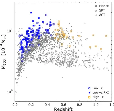
Fig. 1. Distribution in the mass–redshift plane of all the clus-ters published in the Planck, SPT, and ACT catalogues. Filled cir-cles: Planck clusters with available redshifts (Planck Collaboration VIII 2011; Planck Collaboration XXIX 2014; Planck Collaboration XXVII 2016); crosses: SPT (Bleem et al. 2015); plus symbols: ACT (Hasselfield et al. 2013). Masses in the Planck catalogue are derived iteratively from the M500−YSZ relation calibrated using hydrostatic
masses from XMM-Newton; they are not corrected for the hydrostatic equilibrium (HE) bias. In the figure the Planck masses are multiplied by a factor of 1.2 (i.e. assuming 20% bias). The blue and orange open squares identify the Low-z and High-z samples considered in this study (see Sect.2). The clusters that are part of the Low-z PXI sample are shown as filled blue squares.
We adopt a flat Λ-cold dark matter cosmology with Ωm =
0.3,ΩΛ = 0.7, H0 = 70 km Mpc s−1, and h(z) = (Ωm(1+ z)3+
ΩΛ)1/2, where h(z) = H(z)/H
0 throughout. Uncertainties are
given at the 68% confidence level (1σ). All fits were performed via χ2minimisation.
2. The sample
2.1. The high-z SZ-selected sample
Our initial sample is built from the 28 clusters with spectroscopic 0.5 < z < 0.9 in the sample of the XMM-Newton Large Pro-gramme (LP) ID069366 (with re-observation of flared targets in ID72378), consisting of clusters detected at high S /N with Planck, and confirmed by autumn 2011 to be at z > 0.5. The exposure times of these observations were optimised to allow the determination of spatially resolved radial total mass profiles at least up to R500. To extend the redshift coverage to z ∼ 1 we
included the five most massive clusters detected by SPT and Planckin the redshift range 0.9 < z < 1.1. Using deep XMM-Newtonand Chandra observations,Bartalucci et al.(2017,2018) examined the X-ray properties of these objects and determined ICM and HE total mass profiles up to R500. The resulting
obser-vation properties are detailed in Table 1 of Bartalucci et al.
(2017).
Combining the above, we obtain the full ‘High-z’ sample of 33 objects, with MSZ
500 > 5 × 10 14M
, shown with orange
open squares in Fig. 1. The observation details of this sample are detailed in TableB.1.
2.2. The Low-z SZ selected sample
Any evolution study requires a local reference sample with similar selection and quality criteria to act as an ‘anchor’ to compare to high redshifts. The ongoing (AO17) XMM-Newton heritage program ‘Witnessing the culmination of structure for-mation in the Universe’ (PIs M. Arnaud and S. Ettori), based on the final Planck PSZ2 catalogue, will serve this function in the future (observations are to be completed by 2021). In the interim, for the present study we use published XMM-Newton follow-up of Planck-selected local clusters taken from the ESZ sample.
The early SZ (ESZ;Planck Collaboration VIII 2011) cata-logue represents the first release derived from the Planck all-sky SZ survey, containing 188 clusters mostly at z < 0.3. There are a number of studies in the literature describing the X-ray prop-erties of this sample. In particular,Lovisari et al.(2017) charac-terised the global properties and the morphological state of the ESZ clusters covered by XMM-Newton observations. We use their results on the morphological properties of the 118 ESZ clusters at 0.05 < z < 0.5 for which R500is within the field of view, and the
relative error on the morphological parameters is less than 50%. This is about 80% of the corresponding parent ESZ subsample defined with the same z and size criteria, so we do not expect any major bias due to the incomplete XMM-Newton coverage. These objects cover one decade in mass, M500∼[3−20] × 1014M , and
are shown with blue open squares in Fig.1. Henceforth we refer to this sample as the ‘Low-z’ sample.
The spatially resolved thermodynamic properties of an ESZ subsample were analysed by the Planck Collaboration, who combined X-ray and SZ data to calibrate the local scaling relations (Planck Collaboration XI 2011) and measure the pres-sure profiles (Planck Collaboration Int. V 2013). We use the pub-lished thermodynamic profiles of 42 clusters for which R500 is
within the field of view (the subsample ‘A’ defined in Sect. 3.1 of Planck Collaboration XI 2011) to derive the total mass pro-files. These clusters are shown as filled blue squares in Fig. 1. We henceforth refer to this sample as the ‘Low-z PXI’ sample. Its representativeness with respect to the full Low-z sample is excellent, as discussed in AppendixB.
2.3. Data preparation
The observations used in this work were taken using the Euro-pean Photon Imaging Camera (EPIC; Turner et al. 2001 and
Strüder et al. 2001) instrument on board the XMM-Newton satellite. This instrument is composed of three CCD arrays, namely MOS1, MOS2, and PN, which simultaneously observe the target. Datasets were reprocessed using the Science Analysis System3 (SAS) pipeline version 15.0 and calibration files as
available in December 2016. Event files with this calibration applied were produced using the emchain and epchain tools.
The reduced datasets were filtered in the standard fashion. Events for which the keyword PATTERN is <4 and <13 for MOS1, 2, and PN cameras, respectively, were filtered out from the analysis. Flares were removed by extracting a light curve, and removing from the analysis the time intervals where the count rate exceeded 3σ times the mean value. We created the exposure map for each camera using the SAS tool eexpmap. We merged multiple observation datasets of the same object, if available. We report in Table B.1the effective exposure times after all these procedures. We corrected vignetting following the weighting scheme detailed inArnaud et al.(2001). The weight
3 cosmos.esa.int/web/xmm-newton
for each event was computed by running the SAS evigwieght tool on the filtered observation datasets.
Point sources were identified using the Multi-resolution wavelet software (Starck et al. 1998) on the exposure-corrected [0.3−2] keV and [2−5] keV images. We inspected each resulting list by eye to check for false detections and missed sources. We defined a circular region around each detected point source and excised these from the subsequent analysis.
We also defined regions encircling obvious sub-structures. Identified by eye, these regions were considered in the morpho-logical analysis because the parameters we used to characterise the morphological state of a cluster (Sect.4) are sensitive to the presence of any such sub-structure. However, these regions were excluded in the radial profile analysis detailed in Sect.3.
X-ray observations are affected by instrumental and sky backgrounds. The former is due to the interaction of the instru-ment with energetic particles, while the latter is caused by Galac-tic thermal emission and the superimposed emission of all the unresolved point sources, namely the cosmic X-ray background (Lumb et al. 2002;Kuntz & Snowden 2000). These components were estimated differently for the radial profile 1D analysis and for the morphological 2D analysis, as described in Sects.3and4, respectively.
3. Radial profile analysis
3.1. Instrumental background estimation
We evaluated the instrumental background for the radial profile analysis following the procedures described inPratt et al.(2010). Briefly, observations taken with the filter wheel in CLOSED position were renormalised to the source observation count rate in the [10−12] and [12−14] keV bands for the EMOS and PN cameras, respectively. We then projected these event lists in sky coordinates to match our observations. We applied the same point source masking and vignetting correction to the CLOSED event lists as for the source data. We also produced event lists to estimate the out-of-time (OOT) events using the SAS-epchain tool.
3.2. Density and 3D temperature profiles
To determine the radial profiles of density and temperature of the ICM we followed the same procedures and settings detailed in Sects. 3.2 and 3.3 ofBartalucci et al.(2017). Briefly, we firstly determined the X-ray peak by identifying the peak of the emis-sion measured in count-rate images in the [0.3−2.5] keV band smoothed using a Gaussian kernel with a width of between 3 and 5 pixels. We extracted the vignetted-corrected and background-subtracted surface brightness profiles, SX, from concentric
annuli of width 200, centred on the X-ray peak, from both source and background event lists. These profiles were used to derive the radial density profiles, ne(r), employing the deprojection
and PSF correction with regularisation technique described in
Croston et al.(2006).
We obtained the deprojected temperature profiles by per-forming the spectral analysis described in detail inPratt et al.
(2010) and Sect. 3.4 ofBartalucci et al.(2017). The background-subtracted spectrum of a region free of cluster emission was fitted with two unabsorbed MeKaL thermal models plus an absorbed power law with fixed slope of Γ = 1.4. The resulting best-fitting model, renormalised by the ratio of the extraction areas, was then added as an extra component in each annular fit. The cluster emission was modelled by an absorbed MeKaL
model with NH given in TableB.1 using the absorption cross
sections from Morrison & McCammon(1983). Spectral fitting was performed using XSPEC4 version 12.8.2. The deprojected 3D temperature profile, T3D, was derived from the projected
profile using the ‘Non parametric-like’ technique described in Sect. 2.3.2 ofBartalucci et al.(2018).
For the Low-z PXI sample, we used the temperature and den-sity profiles published inPlanck Collaboration Int. V(2013) and
Planck Collaboration XI(2011), which were derived employing identical methods to those used in this work.
3.3. Global properties
We determined the mass at density contrast∆ = 500, MYX
500, and
corresponding RYX
500 radius, from the mass proxy YX. This was
computed iteratively from the M500−YX relation, calibrated by
Arnaud et al.(2010) using HE mass estimates of local relaxed clusters. We assumed that the M500−YX relation obeys
self-similar evolution. The starting mass value was obtained from the M−T relation of Arnaud et al. (2005), and the computa-tion converges typically within 5–10 iteracomputa-tions. The quantity YX
is defined as the product of the temperature measured in the [0.15−0.75]R500region and the gas mass within R500(Kravtsov
et al. 2006), the gas mass profiles being computed from the den-sity profiles. The mass for each cluster and associated errors are reported in TableB.1.
We used the MYX
500 published by Lovisari et al. (2017) for
the Low-z sample, and the MYX
500computed by us for the Low-z
PXI and High-z samples. We investigated the coherence between these measurements by comparing the masses for the clusters in common between the Low-z plus High-z samples and the Low-z PXI sample. The excellent agreement between the two is dis-cussed in Appendix A, and the comparison is shown the right panel of Fig.A.1.
3.4. Derivation of the total mass profiles
Under the assumption that the ICM is in hydrostatic equilibrium in the gravitational potential well the relation between the total halo mass within radius R and the ICM thermodynamic proper-ties is: M(≤ R)= −kT(R) R GµmH " d ln ne(R) d ln R + d ln T (R) d ln R # , (1)
where G is the gravitational constant, mHis the hydrogen atom
mass, and µ = 0.6 is the mean molecular weight in atomic mass unit. We used the deprojected density and temperature profiles and the relation in Eq. (1) to derive the mass profiles, applying the ‘forward non-parametric-like technique’ detailed in Sect. 2.4.1 ofBartalucci et al.(2018). The ‘forward’ in the tech-nique name is due to the fact that we started our analysis from the surface brightness and projected temperature observables to derive the mass profiles at the end. The ‘non-parametric-like’ refers to the fact that we used a deprojection technique to derive the density and temperature profiles, that is, without using para-metric models.
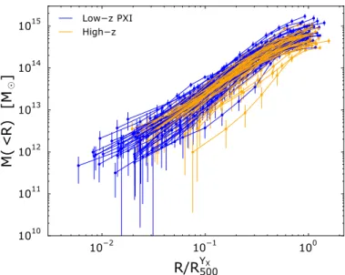
The mass profiles of the Low-z PXI and High-z samples and their associated uncertainties are shown in Fig.2(those of the five highest-redshift clusters are reproduced as published in
Bartalucci et al. 2018). The profiles of the High-z clusters are
4 https://heasarc.gsfc.nasa.gov/xanadu/xspec/
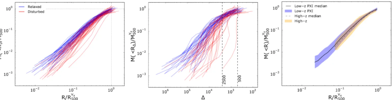
Fig. 2.Integrated mass profiles as a function of scaled radius, estimated from the hydrostatic equilibrium equation, for all clusters considered in this work. The Low-z PXI and High-z samples are plotted in blue and red, respectively.
mapped at least up to 0.8R500, with 20 out of 33 objects
mea-sured up to R500, thus not requiring extrapolation to compute the
HE mass at a density contrast of∆ = 500, MHE
500. The median
sta-tistical error is about 20%. The quality of the Low-z PXI mass profiles, based on archival data, is lower and less homogeneous. Only 18 out of 42 clusters have temperature profiles extending to R500, with a maximum radius between 0.6R500 and 1.4 R500.
Bartalucci et al.(2018) showed that while the HE mass is very robust when the temperature profiles extend up to R500, the
MHE
500mass is very sensitive to the mass estimation method when
extrapolation is required. This is particularly the case for irregu-lar clusters. To minimise systematic errors, we used MYX
500rather
than MHE
500in the following for all scaling with mass, and for the
computation of the sparsity (see below). The possible impact of this choice on our results is discussed in Sect.7.
3.5. Sparsity
The sparsity, S, was introduced by Balmès et al. (2014) to quantify the shape of the dark matter profile. It is defined as the ratio of the integrated mass at two over-densities, and has the advantage of being non-parametric, as there is no a priori assumption on the form of the profile. The sparsity therefore represents a useful measure when dealing with a population of objects with a wide variety of dynamical states. Another non-parametric approach, advocated by Klypin et al.(2016), con-siders the maximum circular velocity, which is linked to the traditional NFW or Einasto concentration. As the velocity is basically the square root of M(<R)/R, it can also be derived from observations. In practice however, measuring such a maxi-mum is much more difficult than measuring a ratio of integrated masses.
In the following, we concentrate on the sparsity to investigate the shape of the mass profiles, which is defined as:
S∆1,∆2 ≡ M∆1
M∆2, (2)
where M∆ is the mass corresponding to the density contrast∆ and with∆1 < ∆2. We recall that M∆ = M(<R∆), which is the
mass enclosed within R∆, such that M(< R∆)
(4π/3) R3 ∆
= ∆ ρcrit. (3)
Balmès et al.(2014) argue that the general properties of the spar-sity do not depend on the choice of∆1,2as long as the halo is well
defined (i.e.∆1is not too small), and that the interaction between
dark and baryonic matter in the central region can be neglected (i.e.∆2is not too large). We use∆1 = 500 and ∆2 = 2500; the
choice of the latter is further discussed in Sect.6.2.
4. Morphological analysis
4.1. Centroid shift
We produced count images for each camera in the soft band, [0.3−2] keV, binned using 200 pixel size, on which we excised
and refilled the masked regions where point sources were detected using the Chandra interactive analysis of observation (CIAO; Fruscione et al. 2006) dmfilth tool. Sub-structures were not masked for this analysis. We estimated the background following a similar approach to that ofBöhringer et al.(2010). We computed the background map for each camera by fitting the refilled count images using a linear combination of the vignetted and unvignetted exposure maps to account for the instrumental and sky background, respectively. We removed the cluster emis-sion by masking a circular region within RYX
500and centred on the
X-ray peak. Exposure maps and background and count images of MOS1, MOS2, and PN were combined, weighting by the ratio of integrated surface brightness profile of each individual cam-era to that of the combined profile. The combined count images were then background subtracted and exposure corrected. We produced 100 realisations of the count-rate maps by applying the same procedure to 100 Poisson realisations of the count maps.
The centroid shift parameter, hwi, was introduced byMohr et al.(1993) as a proxy to characterise the dynamical state of a cluster. The centroid (xc, yc) within an aperture is defined as
(xc, yc) ≡ 1 Ni X k nk(xk; yk), (4)
where Niis the total number of counts per second within the ith
aperture and nk is the count rate in the pixel k of coordinates
(xk; yk). We computed the mean deviation of the centroid from
the X-ray peak by measuring the displacement within N = 10 apertures using the definition ofBöhringer et al.(2010) :
hwi = 1 N −1 10 X i=0 (∆i− h∆i)2 1/2 1 RYX 500 , (5)
where∆i is the projected distance between the X-ray peak and
the centroid computed within the ith concentric annulus, each one being i × 0.1RYX
500in width. Uncertainties on the centroid shift
were estimated by measuring hwi on the 100 Poisson count map realisations, and taking the values within 68% of the median.
Maughan et al.(2008) measured hwi on a sample of clusters observed by Chandra, excluding the inner 30 kpc to make the parameter less sensitive to very bright cores. The PSF of XMM-Newtonis larger for all the clusters considered in this work and, for this reason, we did not excise the core from the analysis. The good agreement between the hwi values derived at z > 0.9 by Chandraand XMM-Newton shown byBartalucci et al.(2017) indicates that the XMM-Newton PSF is not an issue.Nurgaliev et al.(2013) showed that the centroid shift can be biased high in
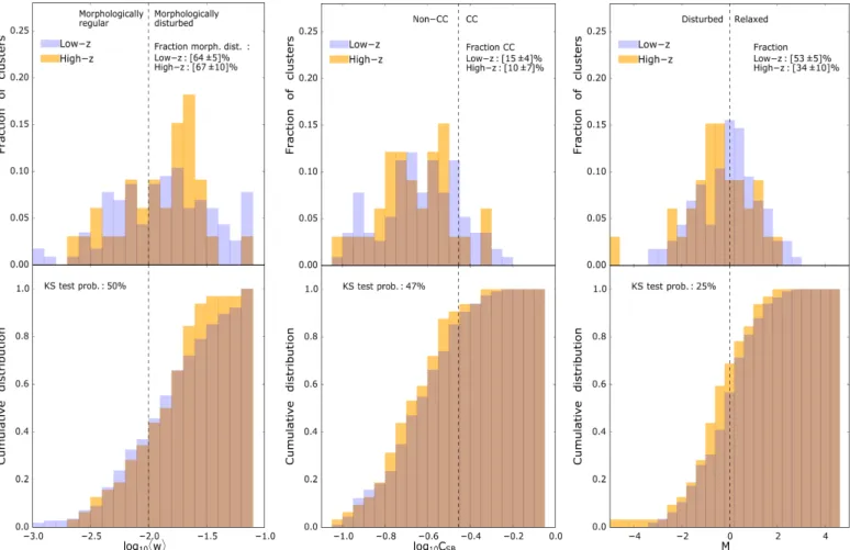
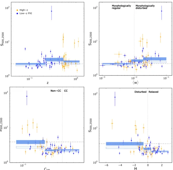
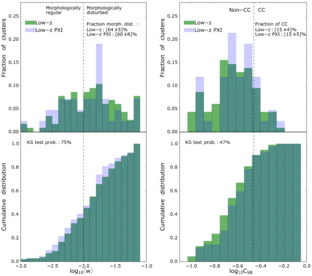
the case of observations with a low number (<2000) of counts. In our sample the minimum number of counts in the [0.3–2] keV band we used to measure hwi is 3000. Furthermore, all clusters are in the high-SN regime, the lowest SN in our sample being 40. FollowingPratt et al.(2009), we initially classify an object as ‘morphologically disturbed’ if hwi > 0.01 and ‘morpholog-ically regular’ if hwi < 0.01 . The results of the centroid shift characterisation for the Low-z and High-z samples is shown in the top- and bottom-left panels of Fig.3, and the corresponding values are given in TableB.1.
4.2. Surface brightness concentration CSB
The ratio of the surface brightness profile within two concen-tric apertures, hereafter the CSB, was introduced bySantos et al.
(2008) to quantify the concentration of cluster X-ray emission. We computed the CSBusing the following definition:
CSB= R0.1×RYX500 0 SX(r) dr R0.5×RYX500 0 SX(r) dr , (6)
where the error was computed using a Monte-Carlo procedure on 100 Gaussian realisations of the surface brightness profiles and taking the 68% value around the median. The CSBparameter
is a robust X-ray measurement, as it relies on the extraction of surface brightness profiles only and is not model-dependent. We nonetheless corrected for the XMM-Newton PSF in view of the high z and small angular size of the high z sample.
Santos et al. (2010) demonstrated that for objects at high redshift the emission within two apertures requires a different k-correction due to the presence of a cool core, that is cool cores will have typically a softer spectrum than the surrounding regions. This correction is potentially important for this study, as we are comparing CSBin a wide redshift range.Santos et al.
(2010) proposed a correction for this effect which requires spa-tially resolved temperature profiles. At the median redshift of the Low-z sample, the k correction is negligible (<1%), but it can be up to ∼5% at the highest redshifts. We therefore did not make this correction for the Low-z sample. For the High-z sam-ple, we applied the k-correction to the CSBof all the clusters as if
they were observed at the median redshift of the Low-z sample, z= 0.19. Henceforth, all the CSBvalues shown and used in this
work are k-corrected in this manner. The results of the CSB
anal-ysis are reported in the top and bottom central panels of Fig.3
and in TableB.1.
The CSBallows the identification of cool-core (hereafter CC)
clusters, the parameter being tightly correlated with the cooling time (e.g.Croston et al. 2008;Santos et al. 2010;Pascut & Ponman 2015). From the correlation between central density and cooling time in theREXCESSsample,Pratt et al.(2009) defined a central density of ne,0 = 0.04 cm−3h(z) as a threshold which segregates
CC and non-CC clusters (their Fig. 2). We computed the central density for the Low-z PXI and High-z objects and used the cor-relation between this quantity and the CSBto translate this
den-sity threshold in terms of the CSB, finding that CC clusters have
CSB> 0.35 for this classification scheme.
The CSBvalue can also be used as an indicator of the
relax-ation state of the cluster. A high concentrrelax-ation is an indicrelax-ation that the core has not been disturbed by recent merger events. The corresponding threshold defined to distinguish relaxed clusters, for example from the anti-correlation observed between hwi and CSBand/or visual inspection (Cassano et al. 2010;Lovisari et al.
Fig. 3.From left to right, normalised histogram (top panels) and cumulative distributions (bottom panels) of the centroid shift, hwi, the concen-tration CSB, and the M parameter (Eq. (7)). The CSBof the High-z sample has been k-corrected as described in Sect.4.2. The Low-z and High-z
distributions are shown in blue and orange, respectively. The vertical dotted line represents the threshold value for each parameter. Left panel: hwi = 0.01 threshold, separating morphologically regular and disturbed clusters. Central panels: CSB= 0.35 threshold, between cool core (CC)
and non-CC objects. Right panels: M= 0 threshold, between disturbed and relaxed objects. The corresponding fraction above each threshold is given in the top right of each figure. In the bottom panels, we report the p-value of the null hypothesis (i.e. that the two distributions are drawn from the same distribution) from the Kolmogorov–Smirnov (KS) test. The distribution of morphologically disturbed and CC objects, based on the parameter hwi and CSB, are not statistically different in the High-z and Low-z samples. However, the combination of the two parameters, M,
indicates that the fraction of disturbed objects is significantly higher in the High-z sample.
4.3. Combined dynamical indicator, M
The combination of certain morphological parameters has been shown to identify the most disturbed and relaxed clusters (Cassano et al. 2010; Rasia et al. 2013; Lovisari et al. 2017;
Cialone et al. 2018). We take advantage of the observed anti-correlation between the centroid shift and the CSB to compute
the M parameter introduced byRasia et al.(2013) and use it as an additional dynamical indicator. M is defined as follows. M ≡ 1
2
CSB− CSB,med
|CSB,quar− CSB,med|
− hwi − hwimed |hwiquar− hwimed|
!
, (7)
where CSB,med and hwimed are the median values of the CSB
and centroid shift, respectively, and CSB,quar and hwquari are
the first or third quartile depending on whether the parameter value is larger or smaller than the median, respectively. The M parameter is therefore an indicator that combines the large-scale (i.e. centroid shift) and the core (i.e. concentration) properties. It is interesting to note that the two morphological parameters appear in Eq. (7) with the same weight to distinguish relaxed and disturbed objects. This is consistent with what has been derived byCialone et al. 2018. According to this definition, clus-ters which are characterised by the presence of a cool core and
are morphologically regular will have M > 0 and very disturbed objects with a very diffuse core will have M < 0.
Henceforth, we refer to the former and latter objects as ‘relaxed’ and ‘disturbed’, respectively. The choice of this dual classification is arbitrary and does not correspond to a strict seg-regation between two types of objects. The distribution of M both for Low-z and High-z samples is continuous, as shown in the top right panel of Fig.3. The results of the M characterisa-tion are reported in the top- and bottom-right panels of Fig.3
and in Table B.1. We note that the numerical value of CSB,med
that we use is smaller than the threshold used in Sect.4.2 to define CC clusters, and is closer to the value chosen byLovisari et al.(2017) after visual classification of clusters when defining a similar M parameter5.
4.4. Consistency of the morphological characterisation We used the results of the morphological analysis published in Lovisari et al. (2017) to characterise the Low-z cluster
5 C
SB,med = 0.23 which is close to CSB = 0.15, used byLovisari et al.(2017), after correction for the different aperture definition (their Fig. C1).
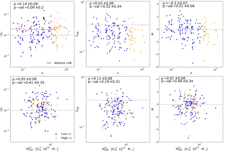
Fig. 4.Morphological parameters vs. redshift (top panel) and mass (bottom panel) of all the clusters used in this work. High-z and Low-z sample clusters are colour-coded in blue and orange, respectively, following the sample colour code of Fig.3. Left panels: centroid shift, hwi. The solid red line is the mean hwi derived byJeltema et al.(2008) from numerical simulations. The dotted lines correspond to the ±68% dispersion, Middle panel: concentration, CSB. Right panel: M parameter. In each panel, the horizontal dotted line identifies the corresponding threshold, as defined in
Fig.3. The symbols ρ and p-value correspond to the Spearman’s rank correlation factor and the corresponding null hypothesis p-value, respectively. Errors on these quantities are computed through 1000 bootstrap resampling. The figure corroborates the lack of evolution with redshift of hwi and CSBshown in Fig.3. However, there is a mild but significant evolution of the combined parameter M. There is no dependence on mass of the
morphological parameters.
morphological properties, using their hwi and CSB values to
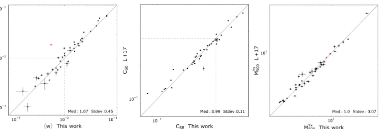
derive the M parameter. We obtained the morphological param-eters of the High-z sample using a different pipeline and differ-ent analysis settings. To avoid potdiffer-entially biased conclusions on morphological evolution or the dependence of the mass profiles on morphology for the full sample, it is necessary to check the consistency between our morphological analysis and that of
Lovisari et al. (2017). We thus compared the morphological parameters derived from each pipeline independently for the common clusters of the Low-z PXI sample. The agreement is excellent, as shown in the left and central panel of Fig.A.1. Full details of the comparison are discussed in AppendixA.
5. Morphology and dynamical state
5.1. Sample characterisation and comparison
The results of the Low-z and High-z morphological characterisa-tion are shown in Fig.3, where the top and bottom of each panel show the normalised and cumulative distribution for each param-eter, respectively. We also show the fraction of objects above the fiducial thresholds discussed in Sect.4.1in each panel. Errors are computed from 1000 Monte-Carlo bootstrap resamples. They
are dominated by the number of clusters, the individual uncer-tainties being much smaller than the intrinsic dispersion.
The top left panel shows that both samples contain a major-ity of disturbed (hwi > 0.01) objects. The shape of the dis-tributions differs, the High-z sample having a prominent peak of objects around hwi ∼ 0.02. This is reflected in the cumula-tive distribution, where there is an excess of High-z objects at log10hwi ∼ −1.4. However, the fraction of disturbed objects in the Low-z sample (64 ± 5%) is nearly identical to that in the High-z sample (67 ± 10%), and is consistent within the uncer-tainties. We investigated if the two samples are representative of the same population by performing the Kolmogorov–Smirnov (KS) test. We determine the p-value of the null hypothesis, that is the two samples are drawn from the same distribution. The p-value is 50%, indicating no significant difference between the Low-z and High-z samples.
We obtained similar results studying the distribution of CC clusters using the CSBparameter, as shown in the central panels
of Fig.3. The fraction of CC clusters is low. The High-z sample has a slightly lower fraction of CC objects (10±5%) as compared to the Low-z sample (15 ± 4%), but the difference is not signifi-cant. Consistently, the KS test yields a high p-value of 47%.
Fig. 5.Scaled radial mass profiles extracted assuming hydrostatic equilibrium for the samples considered in this work. Left panel: radius and mass are scaled by RYX
500and M YX
500, respectively. Blue and red profiles represent relaxed and disturbed objects, respectively, according to the M parameter.
Central panel: same as the left panel, except for the fact that we show the mass profile as a function of the density contrast,∆. The vertical line ∆ = 2500 is the overdensity used in this work to compute the sparsity described in Sect.6. Right panel: comparison of the scaled mass profiles for the Low-z PXI and High-z samples. The solid line and dotted lines represent the median computed for the Low-z PXI and High-z samples, respectively. The gold and green shaded regions represent the 1σ dispersion of the Low-z PXI and High-z samples, respectively. Disturbed clusters have a shallower mass distribution, and present a larger dispersion than that of the most relaxed objects. On the other hand, the median HE mass profile depends mildly on redshift.
Interestingly, the M distributions shown in the right panels of Fig.3suggest some evolution. While the distributions have qual-itatively similar shapes, the High-z sample has a peak which is clearly shifted towards disturbed objects. Furthermore, the frac-tion of relaxed clusters in the Low-z sample, 53 ± 5%, is 50% higher than that of the High-z sample, 34 ± 8%, a 2σ effect. This evolution can be seen in the cumulative distribution as a system-atic over-abundance of disturbed objects in the High-z sample as compared to the Low-z PXI sample. The KS test yields a smaller p-value of 25%, but this is not small enough to reject the null-hypothesis.
5.2. Mass dependence and redshift evolution
For each morphological parameter, we further quantified the relation with mass and redshift by computing the Spearman’s rank (SR) coefficient ρ and the null hypothesis p-value, the prob-ability that the observed coefficient is obtained by chance if the two parameters are completely independent. We also considered the sum square difference of ranks, D, and the number of stan-dard deviations by which D deviates from its null-hypothesis expected value, σD. As in the previous section, we performed
1000 bootstrap resamples to estimate these values and their 68% errors. The top and bottom panels of Fig. 4show each param-eter as a function of redshift and mass, respectively. The cen-troid shift, CSB, and M parameters are shown in the left, middle,
and right panels, respectively, with the SR coefficient and corre-sponding p-value indicated in the top left of each plot.
The only parameter for which there is a correlation with z is the combined M parameter, for which ρ = −0.2 ± 0.1. The correlation is not very significant, with a null-hypothesis p-value of 0.01 ± 0.07, and a standard deviation on the null hypothesis of σD = 2.5 ± 1. The Kendall test gives consistent results. This
weak correlation of M with z comes from the amplification of the positive (but not significant) trend in hwi versus z, while there is no correlation between CSBand redshift.
In summary, consistent with the trend observed in Sect.5.1
above, there is weak evidence that clusters at higher redshift are slightly more disturbed. On the other hand, there is no evidence for any trend with mass, the SR coefficient for all parameters being consistent with zero and the corresponding p-value in the range 20%–50%. This is in agreement with the mass
indepen-dence of the dynamical state found byBöhringer et al. (2010) andLovisari et al.(2017) for local clusters. We must note how-ever that the mass range is limited in the present sample.
6. Total mass profile shape
6.1. Radial mass profiles
The individual scaled HE integrated total mass profiles are shown in Fig.5. In the left and central panels, the profiles are colour coded according to their morphological state according to the M parameter: in blue for the relaxed (M > 0) and in red for the disturbed (M < 0) clusters.
There is a clear difference between the two populations in the [0.01−0.5]RYX
500range. As compared to the relaxed clusters,
the disturbed objects have a shallower mass distribution on aver-age (i.e. there is less mass within the central region), and these profiles show a larger dispersion. This effect is even more evi-dent in the central panel of Fig.5, where the mass profiles are plotted as a function of the total density contrast,∆. As ∆ is pro-portional to the mean total density within a sphere of radius R∆ (Eq. (3)), it decreases with radius, more or less rapidly depend-ing on the steepness of the density profile. For density profiles that are very peaked towards the centre,∆ decreases rapidly, or equivalently M (<R∆) slowly increases with decreasing ∆. On the other hand, a flat profile within the core would correspond to a constant mean density, thus quasi-constant∆, and a very steep variation of M (<R∆) with∆ in the central region, with a maxi-mum value of∆ corresponding to that of the core. This is what is observed for the relaxed and disturbed clusters, respectively. In summary, the dynamical state of the cluster clearly has a very strong impact on the shape of the total mass profile.
The right panel of Fig.5shows the 68% dispersion envelopes of the Low-z PXI and High-z samples with light and dark green, respectively. The black solid and dotted lines represent the median profiles for the Low-z PXI and High-z samples, respec-tively. The envelopes of the two samples are consistent. How-ever, the median HE mass profile of the High-z sample is slightly lower and shallower than that of the Low-z PXI sample, being lower by 6.5% and 16% at 0.9RYX
500 and 0.3R YX
500, respectively.
The HE radial mass profiles thus show a hint of evolution, but this is not statistically significant considering the dispersion of
Fig. 6.Top left panel: sparsity of the Low-z PXI and High-z samples as a function of redshift. The filled blue rectangles represent the mean sparsity weighted by the statistical errors and the intrinsic dispersion, estimated iteratively (see text), and its 1σ uncertainty. This is computed in three bins, defined to have approximately the same number of objects (see Table1). The open blue rectangles represent the same quantity computed removing the outliers. We show as reference the median value of the first bin with the black dotted line. Top right panel: same but with the sparsity as a function of hwi. Bottom left panel: same but with sparsity as a function of the CSB. Bottom right panel: same but with the sparsity as a function
of M. The sparsity, i.e. the shape of the total mass profile, varies significantly with the dynamical state indicators. More disturbed clusters have higher sparsity i.e. they are less concentrated. The dependence on redshift is smaller than the dependence on the dynamical state.
the profiles. Interestingly, the dispersions of the two samples are similar. We recall that the samples contain a similar number of objects, the Low-z PXI and High-z having 42 and 33 objects, respectively, and the data quality ensures that HE mass profiles are computed for each object. In view of our finding above that the morphology evolution is negligible, the absence of evolution of the HE mass profile dispersion is a natural consequence of their shape being driven by the dynamical state.
6.2. The shape of the mass profiles
We further quantified the evolution and the impact of dynamical state on the shape of the profile using the sparsity, S500/2500. We
chose∆2= 2500, which is large enough to encompass the
depen-dence of the mass profile shape as a function of the dynamical state and is reached by all haloes, as shown in the middle panel of Fig.5.
Figure6shows the sparsity as a function of the redshift in the top-left panel, and the three morphological parameters, hwi,
CSB, and M in the top-right, bottom-left, and bottom-right
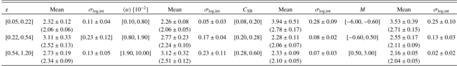
pan-els, respectively. The statistical errors on the sparsity are not negligible as compared to the intrinsic scatter, and the simple correlation tests used in the previous section cannot be applied. We therefore computed the mean sparsity in bins. We defined three bins in redshift and for each parameter, the width of each bin being defined so as to have roughly the same number of objects in each bin. The logarithmic mean of the sparsity was computed in each bin, weighting each value by the quadratic sum of the statistical error and the intrinsic scatter. This scatter and the weighted mean were estimated simultaneously by iteration. The mean and intrin-sic scatter, together with their 68% errors, were computed using 1000 bootstrap resamples. The results are reported in Table1and as filled blue rectangles in each panel of Fig.6. As there is a large scatter with the presence of strong outliers, we also computed the mean within the same bins excluding the >3σ outliers. The results are shown with the open blue rectangles.
There seems to be a slight although not very significant evo-lution of the sparsity with z. Higher-redshift (z > 0.54) clusters
Table 1. Mean values of the sparsity and their uncertainties computed in the bins shown in Fig.6as a function of z, hwi, CSB, and M.
z Mean σlog,int hwi [10−2] Mean σlog,int CSB Mean σlog,int M Mean σlog,int
[0.05, 0.22] 2.32 ± 0.12 0.11 ± 0.04 [0.10, 0.80] 2.26 ± 0.08 0.05 ± 0.03 [0.08, 0.20] 3.94 ± 0.51 0.28 ± 0.09 [−6.00, −0.60] 3.53 ± 0.39 0.25 ± 0.10 (2.06 ± 0.06) (2.06 ± 0.05) (2.78 ± 0.17) (2.71 ± 0.15) [0.22, 0.54] 3.11 ± 0.33 [0.23 ± 0.12] [0.80, 1.90] 2.77 ± 0.23 0.17 ± 0.04 [0.20, 0.28] 2.28 ± 0.11 0.08 ± 0.02 [−0.60, 0.50] 2.55 ± 0.17 0.13 ± 0.03 (2.52 ± 0.13) (2.24 ± 0.10) (2.06 ± 0.07) (2.11 ± 0.09) [0.54, 1.20] 2.73 ± 0.19 0.13 ± 0.05 [1.90, 10.00] 3.12 ± 0.32 0.23 ± 0.11 [0.28, 0.60] 2.33 ± 0.09 0.07 ± 0.03 [0.50, 3.00] 2.16 ± 0.05 0.02 ± 0.02 (2.34 ± 0.09) (2.51 ± 0.12) (2.10 ± 0.05) (2.04 ± 0.05)
Notes. The means are computed in logarithmic space and take into account both statistical errors and the intrinsic dispersion, estimated iteratively. The intrinsic dispersion σlog,intin dex are given in the table. The values between parentheses are the sparsities computed within the same bins
excluding the outliers.
have a slightly larger value of S500/2500 by 18%, that is these
profiles are less concentrated, which is not consistent with the low-redshift (z < 0.2) clusters at ∼1.8σ. We found the same behaviour when excluding the outliers.
There is a much stronger and significant variation of the spar-sity with dynamical state: morphologically disturbed (high hwi), non-CC (low CSB), and disturbed (low M) clusters have larger
sparsity. For all parameters considered, the sparsity of the first and third bins is not consistent at more than 3σ, and the dif-ference between the sparsities of these bins is of the order of ∼50%. At the same time, the intrinsic scatter increases signifi-cantly, reaching ∼0.2 dex for the most disturbed or least concen-trated objects. For example, the sparsity increases by 64% at a significance level of 3.4σ between M < −0.6 and M > 0.5, that is, between the one third most relaxed and the one third most dis-turbed as defined by this parameter. Only an upper limit on the intrinsic scatter can be estimated from the former (<0.04 dex), while the intrinsic scatter for the latter reaches 0.25 ± 0.09 dex. There are strong outliers at high sparsity. Excluding the out-liers yields the same qualitative results, although the variation between bins is weaker. This suggests a sparsity distribution skewed towards high values, with a skewness increasing with departure from dynamical relaxation.
7. Discussion
7.1. Dynamical state
The first result of our study is that SZ-selected samples are dom-inated at all redshifts by disturbed and non-CC objects. Recent observational work on local clusters has converged to similar results (e.g.Lovisari et al. 2017;Rossetti et al. 2017; Andrade-Santos et al. 2017;Lopes et al. 2018). In particular, these works highlight the higher fraction of disturbed objects or the lower fraction of CC objects in SZ-selected samples as compared to X-ray-selected samples, a fact interpreted to be due to preferen-tial detection of relaxed or more concentrated clusters in X-ray surveys.
In contrast, there is little consensus in the literature concern-ing the evolution of the dynamical state, as determined from var-ious morphological parameters. Studies of the evolution up to z ∼1 of the centroid shift and/or power ratios of X-ray-selected clusters indicate a larger fraction of disturbed clusters at high z (Maughan et al. 2008; Jeltema et al. 2005; Weißmann et al. 2013). However, the latter study is also consistent with no evo-lution, andNurgaliev et al.(2017) did not find any significant evolution in the redshift range 0.3 < z < 1 for the 400 d X-ray-selected clusters.
These somewhat contradictory results may simply be due to selection effects: X-ray detectability is clearly not independent of
cluster morphology. More peaked clusters (usually relaxed) are not only more luminous at a given mass, but are also easier to detect at a given X-ray luminosity. Such effects are particularly important in flux-limited surveys, as shown byChon & Böhringer
(2017) in the context of a volume-limited X-ray survey. It is there-fore difficult to disentangle selection effects and/or z and mass dependence (see also the discussion inMantz et al. 2015).
Sunyaev–Zeldovich detection does not suffer from these lim-itations, and an SZ-selected sample is expected to be close to mass-limited. The morphological evolution of SPT clusters was studied recently by Nurgaliev et al. (2017) using their newly introduced aphotparameter. They did not find a significant
dif-ference between the redshift ranges [0.3–0.6] and [0.6–1.2]. This absence of significant evolution was also observed byMcDonald et al.(2017) up to z= 1.6, also for an SPT sample. The compre-hensive study of classification criteria for the most relaxed clus-ters byMantz et al.(2015) indicates that the fraction of relaxed clusters in the SPT and Planck samples is consistent with being constant with redshift.
In the present study, we extend the morphological analysis of the full SZ-selected population of high-mass clusters, from very local systems z = 0.05 up to z = 1, applying a consistent sam-ple construction and analysis strategy over the full z range. The high quality of our data allows us to investigate core (i.e. CSB)
and bulk (i.e. hwi) properties at high precision. There are no sig-nificant trends either with z or mass in these parameters individ-ually. However, we find a significant evolution with z of the M dynamical indicator, which combines these large-scale and core parameters, with a null-hypothesis p-value of 1%.
It has been suggested that the fraction of disturbed clus-ters should increase with z and mass in a hierarchical formation model (e.g. Böhringer et al. 2010; McDonald et al. 2017). To explain the observed absence of evolution in the SPT sample,
McDonald et al.(2017) proposed a simple model, combining the merger rate from the simulations ofFakhouri et al.(2010) and a fiducial relaxation time of the hot gas equal to the crossing time. In fact, the link between cluster formation history and morphologi-cal state as observed in X-rays, as a function of z and mass, is very complex. This first depends on relating the individual mass assem-bly history to dynamical state (e.g.Power et al. 2012), and then the dynamical state to morphological indicators (e.g.Cui et al. 2017). Individual cluster history is never observed directly and has to be translated into the ensemble properties of cluster sam-ples at different z (e.g. seeMostoghiu et al. 2019). A further com-plication is the relation between the gas dynamical history and that of the underlying dark matter, and how X-ray morphological observables relate to the gas dynamical state. To our knowledge the only theoretical prediction of the evolution of observed ICM morphological parameters is that ofJeltema et al.(2008). These latter authors claim a significant evolution of the mean hwi with
z, although a comparison of their results with our data in Fig.4
shows that any such evolution is mild, is much smaller than the dispersion, and is fully in agreement with our results.
7.2. Total mass profile
Extending the pilot study ofBartalucci et al.(2018) with a fully SZ-selected sample, the overall picture emerging from the pre-sent work is that the shape of the dark matter profiles is affected both by evolution and by dynamical state (Table1). The evolu-tion effect is mild, increasing the sparsity of objects by ∼15% from z ∼0.1 to z ∼ 0.8. In contrast, the M dependence is much stronger, with a sparsity increasing by ∼60% with decreasing M, that is from the most relaxed to the most disturbed objects. This varia-tion of profile shape with dynamical state is likely a fundamental property, rather than a secondary consequence of the mutual var-iation of the S500,2500 and M parameters with z, which are both
less significant. A multi-component analysis requiring a larger sample is needed to firmly assess this point.
An obvious question is whether the observed dependence of the sparsity on dynamical state is an artefact of systematic error in the X-ray mass estimate. As discussed in detail by
Corasaniti et al.(2018) the sparsity derived from HE mass esti-mates is essentially bias-free (less than 5%). As it is a mass ratio, the sparsity is only sensitive to the radial dependence of any bias, which is usually small between the density contrasts under con-sideration. The mean S500,2500bias from the HE mass estimate for
example is of ∼3.2% from the simulations ofBiffi et al.(2016). Generally, although the exact radial dependence of the HE bias will differ from object to object, we expect it to increase towards larger radii (smaller∆) meaning that sparsity S500/2500measured
from HE profiles would be biased low as compared to the true value, especially for the most disturbed objects. This effect is the opposite to the observed increase of sparsity for increasingly perturbed systems. As detailed in Sect. 3.5we are not directly using the HE mass at∆ = 500 but its proxy, MYX
500. For the
clus-ters for which no extrapolation is needed, the differences between these measures are the order of 10%, with no systematic trend with dynamical state. Thus, the measured sparsity may be slightly lower than if we had used the HE mass, but the clear trend of the sparsity with dynamical state would not be changed.
The trend of sparsity with dynamical state indicates that mor-phologically disturbed objects are less concentrated than relaxed objects. There is also evidence for increased scatter. This is qual-itatively in agreement with the difference in the c–M relations for relaxed versus disturbed objects seen in numerical simulations (e.g.Bhattacharya et al. 2013, Figs. 1 and 4). InLe Brun et al.
(2018) we performed a preliminary investigation using numeri-cal simulations tailored to cover the high-mass high-z range con-sidered here. In these simulations, the sparsity of the 25 most massive clusters at all redshifts shows a correlation with the DM dynamical indicator∆r6with a p-value of [0.5−2]% (their Fig. 3), indicating that sparser clusters are less regular. We will revisit the link between dynamical state and DM sparsity for the full simulated sample in a forthcoming paper.
8. Conclusions
We present new XMM-Newton observations of a Planck SZ-selected sample of 28 massive clusters in the redshift range z = [0.5−0.9]. These were combined with the sample of
6 ∆r is defined as the distance between the centre of mass and the
centre of the shrinking sphere (Le Brun et al. 2018).
Bartalucci et al.(2018) at 0.9 < z < 1.1 for a total High-z sample of 33 objects at masses MYSZ
500 > 5 × 10 14M
. We characterised
the dynamical state with the centroid shift hwi, the concentra-tion CSB, and the combination of the two parameters, M, which
simultaneously probes the large-scale and core morphology. The shape of the total mass profile, derived from the hydrostatic equi-librium equation, was quantified using the sparsity, the ratio of M500 to M2500, that is the masses at density contrast 500 and
2500, respectively. This parameter, introduced byBalmès et al.
(2014) offers a non-parametric measurement of the shape which is thought to be relatively insensitive to HE bias (Corasaniti et al. 2018) .
We first combined the High-z morphology measurements with those of the ESZ clusters at z < 0.5 inLovisari et al.(2017), for a total sample of 151 objects. In this study:
– We confirmed that SZ-selected samples, thought to best reflect the underlying cluster population, are dominated by disturbed (∼65%) and non-CC (∼80%) objects, at all red-shifts.
– There is no significant evolution or mass dependence of the fraction of cool core or of the centroid shift parameter. The only parameter for which there is a significant correlation with z is the combined M parameter, for which ρ= −0.2±0.1 and a null-hypothesis p-value of 0.01.
We then combined the mass measurements obtained for our new data with those from a subsample of 42 ESZ objects with spa-tially resolved ICM profiles presented in Planck Collaboration Int. V(2013), and which we confirmed is representative of the full Low-z sample. The total sample of 75 objects covers the red-shift range 0.08 < z < 1.1 and mass range [5−20] × 1014M
. We
made the following findings.
– The median scaled mass profile differs by less than 6.5% and 16% at 0.9RYX
500and 0.3R YX
500, respectively, between the Low-z
PXI and High-z samples, with no difference in the dispersion. The evolution of the sparsity with z is mild: it increases by only 18% between z < 0.2 and z > 0.55, an effect significant at less than 2σ.
– When expressed in terms of a scaled mass profile, there is a clear difference between relaxed and disturbed objects. The latter have a less concentrated mass distribution on average, and their scaled profiles show a much larger dispersion. – Consequently there is a clear dependence of the sparsity on
the dynamical state. When expressed as a function of the M parameter, the sparsity increases by ∼60% from the one third most relaxed to the one third most disturbed objects, an effect significant at more than 3σ level. We discussed the fact that the HE bias will not significantly change this result.
The main result of this work is that the radial mass distribution is chiefly governed by the dynamical state of the cluster and only mildly dependent on redshift. This has important consequences: – A coherent sample selection at all z is key. For instance, one cannot compare the c–M relation calibrated at low z on the most relaxed X-ray selected clusters to that of a SZ-selected sample at high z. Ideally, one should consider complete sam-ples, representative of the full true underlying cluster pop-ulation; for example, a mass-selected sample. This is even more critical when comparing theory and observation, in view of the difficulty of defining coherent dynamical indi-cators between the two.
– To test theoretical predictions, it is insufficient to simply compare median or stacked properties at each z. The dis-persion is a critical quantity, as is the profile distribution, in view of likely departure from log-normality. This requires the measurement of individual profiles. X-ray observations
currently provide the best way to obtain such profiles at high statistical precision.
– In view of this, observational and theoretical efforts to under-stand the HE bias and its radial dependence are all the more important.
In a forthcoming paper, we will extend our study of the depen-dence of the sparsity on the dynamical state using an extension of the dark matter simulations presented inLe Brun et al.(2018) to a larger sample of clusters at M500> 5 × 10¹⁴M . On a longer
timescale, the link between the true dark matter distribution and its dynamical state and the X-ray observables will need to be better understood. This includes the link between ICM morpho-logical proxies and the true underlying dynamical state, and the potential critical issue of the radial variation of the HE bias. We will address these issues with dedicated simulations.
On the observational side, we will investigate the HE bias by comparing our results to weak lensing mass measurements for a subsample of the present data set. The observed lack of signif-icant evolution needs to be tested with a larger sample, particu-larly at z > 0.7 where the present sample is limited, with data of the same or better quality. The fundamental link uncovered by the present paper between the mass profile and dynamical state will also need to be consolidated with better Low-z data. Our cur-rent Low-z sample relies on archival data of uneven quality and is not a complete sample. The building of a new local reference SZ-selected sample, with high-quality ICM thermodynamic and HE mass profiles, will be one of the main outcomes of the AO17 XMM-Newtonheritage program ‘Witnessing the culmination of structure formation in the Universe’, and will provide the neces-sary inputs.
Acknowledgements. The authors would like to thank Barbara Sartoris for help-ful comments and suggestions. The results reported in this article are based on data obtained with XMM-Newton, an ESA science mission with instruments and contributions directly funded by ESA Member States and NASA. This work was supported by CNES. The research leading to these results has received funding from the European Research Council under the European Union’s Sev-enth Framework Programme (FP72007-2013) ERC grant agreement no 340519. LL acknowledges support from NASA through contracts 80NSSCK0582 and 80NSSC19K0116.
References
Amodeo, S., Ettori, S., Capasso, R., & Sereno, M. 2016,A&A, 590, A126 Andrade-Santos, F., Jones, C., Forman, W. R., et al. 2017,ApJ, 843, 76 Arnaud, M., Neumann, D. M., Aghanim, N., et al. 2001,A&A, 365, L80 Arnaud, M., Pointecouteau, E., & Pratt, G. W. 2005,A&A, 441, 893 Arnaud, M., Pratt, G. W., Piffaretti, R., et al. 2010,A&A, 517, A92
Balmès, I., Rasera, Y., Corasaniti, P.-S., & Alimi, J.-M. 2014,MNRAS, 437, 2328
Bartalucci, I., Arnaud, M., Pratt, G. W., et al. 2017,A&A, 598, A61
Bartalucci, I., Arnaud, M., Pratt, G. W., & Le Brun, A. M. C. 2018,A&A, 617, A64
Bhattacharya, S., Habib, S., Heitmann, K., & Vikhlinin, A. 2013, ApJ, 766, 32
Biffi, V., Borgani, S., Murante, G., et al. 2016,ApJ, 827, 112 Bleem, L. E., Stalder, B., de Haan, T., et al. 2015,ApJS, 216, 27 Böhringer, H., Pratt, G. W., Arnaud, M., et al. 2010,A&A, 514, A32 Cassano, R., Ettori, S., Giacintucci, S., et al. 2010,ApJ, 721, L82 Chon, G., & Böhringer, H. 2017,A&A, 606, L4
Cialone, G., De Petris, M., Sembolini, F., et al. 2018,MNRAS, 477, 139 Corasaniti, P. S., Ettori, S., Rasera, Y., et al. 2018,ApJ, 862, 40
Correa, C. A., Wyithe, J. S. B., Schaye, J., & Duffy, A. R. 2015,MNRAS, 452, 1217
Croston, J. H., Arnaud, M., Pointecouteau, E., & Pratt, G. W. 2006,A&A, 459, 1007
Croston, J. H., Pratt, G. W., Böhringer, H., et al. 2008,A&A, 487, 431 Cui, W., Power, C., Borgani, S., et al. 2017,MNRAS, 464, 2502
da Silva, A. C., Kay, S. T., Liddle, A. R., & Thomas, P. A. 2004,MNRAS, 348, 1401
Diemer, B., & Kravtsov, A. V. 2015,ApJ, 799, 108
Dolag, K., Bartelmann, M., Perrotta, F., et al. 2004,A&A, 416, 853 Dutton, A. A., & Macciò, A. V. 2014,MNRAS, 441, 3359 Einasto, J. 1965,Trudy Astrofizicheskogo Instituta Alma-Ata, 5, 87 Fakhouri, O., Ma, C.-P., & Boylan-Kolchin, M. 2010,MNRAS, 406, 2267 Fruscione, A., McDowell, J. C., Allen, G. E., et al. 2006,Proc. SPIE, 6270,
62701V
Hasselfield, M., Hilton, M., Marriage, T. A., et al. 2013,JCAP, 7, 008 Jeltema, T. E., Canizares, C. R., Bautz, M. W., & Buote, D. A. 2005,ApJ, 624,
606
Jeltema, T. E., Hallman, E. J., Burns, J. O., & Motl, P. M. 2008,ApJ, 681, 167 Jing, Y. P. 2000,ApJ, 535, 30
Kalberla, P. M. W., Burton, W. B., Hartmann, D., et al. 2005,A&A, 440, 775 Klypin, A., Yepes, G., Gottlöber, S., Prada, F., & Heß, S. 2016,MNRAS, 457,
4340
Kravtsov, A. V., & Borgani, S. 2012,ARA&A, 50, 353 Kravtsov, A. V., Vikhlinin, A., & Nagai, D. 2006,ApJ, 650, 128 Kuntz, K. D., & Snowden, S. L. 2000,ApJ, 543, 195
Le Brun, A. M. C., Arnaud, M., Pratt, G. W., & Teyssier, R. 2018,MNRAS, 473, L69
Lopes, P. A. A., Trevisan, M., Laganá, T. F., et al. 2018,MNRAS, 478, 5473 Lovisari, L., Forman, W. R., Jones, C., et al. 2017,ApJ, 846, 51
Ludlow, A. D., Navarro, J. F., Angulo, R. E., et al. 2014,MNRAS, 441, 378 Lumb, D. H., Warwick, R. S., Page, M., & De Luca, A. 2002,A&A, 389, 93 Mantz, A. B., Allen, S. W., Morris, R. G., et al. 2015,MNRAS, 449, 199 Marriage, T. A., Acquaviva, V., Ade, P. A. R., et al. 2011,ApJ, 737, 61 Maughan, B. J., Jones, C., Forman, W., & Van Speybroeck, L. 2008,ApJS, 174,
117
McDonald, M., Allen, S. W., Bayliss, M., et al. 2017,ApJ, 843, 28 Mohr, J. J., Fabricant, D. G., & Geller, M. J. 1993,ApJ, 413, 492 Morrison, R., & McCammon, D. 1983,ApJ, 270, 119
Mostoghiu, R., Knebe, A., Cui, W., et al. 2019,MNRAS, 483, 3390 Navarro, J. F., Frenk, C. S., & White, S. D. M. 1997,ApJ, 490, 493 Navarro, J. F., Hayashi, E., Power, C., et al. 2004,MNRAS, 349, 1039 Neto, A. F., Gao, L., Bett, P., et al. 2007,MNRAS, 381, 1450 Nurgaliev, D., McDonald, M., Benson, B. A., et al. 2013,ApJ, 779, 112 Nurgaliev, D., McDonald, M., Benson, B. A., et al. 2017,ApJ, 841, 5 Pascut, A., & Ponman, T. J. 2015,MNRAS, 447, 3723
Planck Collaboration VIII. 2011,A&A, 536, A8 Planck Collaboration XI. 2011,A&A, 536, A11 Planck Collaboration XXIX. 2014,A&A, 571, A29 Planck Collaboration XXVII. 2016,A&A, 594, A27 Planck Collaboration Int. V. 2013,A&A, 550, A131
Power, C., Knebe, A., & Knollmann, S. R. 2012,MNRAS, 419, 1576 Pratt, G. W., Croston, J. H., Arnaud, M., & Böhringer, H. 2009,A&A, 498,
361
Pratt, G. W., Arnaud, M., Piffaretti, R., et al. 2010,A&A, 511, A85 Pratt, G. W., Arnaud, M., Biviano, A., et al. 2019,Space Sci. Rev., 215, 25 Rasia, E., Meneghetti, M., & Ettori, S. 2013,Astron. Rev., 8, 40 Reichardt, C. L., Stalder, B., Bleem, L. E., et al. 2013,ApJ, 763, 127 Rossetti, M., Gastaldello, F., Eckert, D., et al. 2017,MNRAS, 468, 1917 Santos, J. S., Rosati, P., Tozzi, P., et al. 2008,A&A, 483, 35
Santos, J. S., Tozzi, P., Rosati, P., & Böhringer, H. 2010,A&A, 521, A64 Starck, J. L., Murtagh, F., & Bijaoui, A. 1998,Image Processing and Data
Analysis: The Multiscale Approach(New York, USA: Cambridge University Press)
Strüder, L., Briel, U., Dennerl, K., et al. 2001,A&A, 365, L18 Turner, M. J. L., Abbey, A., Arnaud, M., et al. 2001,A&A, 365, L27 Velliscig, M., van Daalen, M. P., Schaye, J., et al. 2014,MNRAS, 442, 2641 Weißmann, A., Böhringer, H., & Chon, G. 2013,A&A, 555, A147
Wu, H.-Y., Hahn, O., Wechsler, R. H., Mao, Y.-Y., & Behroozi, P. S. 2013,ApJ, 763, 70
Appendix A: Low-z versus Low-z PXI characterisation
In this work we used the results ofLovisari et al.(2017) to char-acterise the morphological properties of the Low-z sample, using it as anchor for the local universe properties. For this reason, it is mandatory that the morphological parameters we derived for the High-z sample are coherent with the values computed from
Lovisari et al.(2017). We derived the centroid shift, CSB, and
the MYX
500 for the Low-z PXI objects we have in common with
Lovisari et al.(2017). The comparison between these values are shown in Fig.A.1, denoting our andLovisari et al.(2017) values with ‘This work’ and ‘L+17’ labels, respectively. The measure-ments of the centroid shifts shown in the left panel are in good
agreement, with a ratio of 1.07 and a standard deviation of 0.45. The strongest outlier is MACS J2243.3−0935, shown with a red point. The difference is probably caused by the different choice of the X-ray peak (distant by ∼700) amplified by the high ellip-ticity of this object. The concentration parameter CSB and the
masses, shown in the central and right panels, respectively, are in excellent agreement. The median ratio for both quantities is excellent and the dispersion is remarkably small, the two anal-ysis being performed with different pipelines. This comparison shows that the measurements that require larger samples for sta-tistical reasons, such as the centroid shift, are more sensitive to analysis parameters such as the choice of the centre or the exclu-sion of point sources; integrated quantities such as the CSBare
more robust.
Fig. A.1.Left panel: comparison between the centroid shifts computed in this work and published inLovisari et al.(2017) on the x and y axis, respectively. The red points highlight the outlier. The dotted lines indicate the threshold used to discriminate between disturbed and relaxed clusters. The solid line is the identity relation. The median and standard deviation were computed weighting by the errors and excluding the two outliers. Central panel: same as the left panel except that the comparison is done for the CSB. The dotted lines indicate the threshold used to discriminate
between CC and non-CC clusters. Right panel: same as the left panel except that the comparison is done for the MYX