HAL Id: hal-02987628
https://hal.archives-ouvertes.fr/hal-02987628
Submitted on 4 Nov 2020
HAL is a multi-disciplinary open access
archive for the deposit and dissemination of
sci-entific research documents, whether they are
pub-lished or not. The documents may come from
teaching and research institutions in France or
abroad, or from public or private research centers.
L’archive ouverte pluridisciplinaire HAL, est
destinée au dépôt et à la diffusion de documents
scientifiques de niveau recherche, publiés ou non,
émanant des établissements d’enseignement et de
recherche français ou étrangers, des laboratoires
publics ou privés.
Yoshihiro Fujiwara, Hidetaka Nomaki
To cite this version:
Dewi Langlet, Vincent Bouchet, Riccardo Riso, Yohei Matsui, Hisami Suga, et al.. Foraminiferal
Ecology and Role in Nitrogen Benthic Cycle in the Hypoxic Southeastern Bering Sea. Frontiers in
Marine Science, Frontiers Media, 2020, 7, �10.3389/fmars.2020.582818�. �hal-02987628�
doi: 10.3389/fmars.2020.582818
Edited by: Chiara Romano, Spanish National Research Council, Spain Reviewed by: María López-Acosta, Spanish National Research Council, Spain Chiara Borrelli, University of Rochester, United States *Correspondence: Dewi Langlet [email protected]; [email protected]
Specialty section: This article was submitted to Deep-Sea Environments and Ecology, a section of the journal Frontiers in Marine Science Received: 13 July 2020 Accepted: 16 September 2020 Published: 04 November 2020 Citation: Langlet D, Bouchet VMP, Riso R, Matsui Y, Suga H, Fujiwara Y and Nomaki H (2020) Foraminiferal Ecology and Role in Nitrogen Benthic Cycle in the Hypoxic Southeastern Bering Sea. Front. Mar. Sci. 7:582818. doi: 10.3389/fmars.2020.582818
Foraminiferal Ecology and Role in
Nitrogen Benthic Cycle in the
Hypoxic Southeastern Bering Sea
Dewi Langlet1,2* , Vincent M. P. Bouchet2, Riccardo Riso2, Yohei Matsui1, Hisami Suga3,
Yoshihiro Fujiwara4and Hidetaka Nomaki1
1X-star, Japan Agency for Marine-Earth Science and Technology (JAMSTEC), Yokosuka, Japan,2Univ. Lille, CNRS, Univ.
Littoral Côte d’Opale, UMR 8187 – LOG – Laboratoire d’Océanologie et de Géosciences, Station Marine de Wimereux, Lille, France,3Research Institute for Marine Resources Utilization (MRU), Japan Agency for Marine-Earth Science and Technology
(JAMSTEC), Yokosuka, Japan,4Research Institute for Global Change (RIGC), Japan Agency for Marine-Earth Science
and Technology (JAMSTEC), Yokosuka, Japan
Southeastern Bering Sea is one of the highest surface productivity area in the open ocean due to strong upwelling along the Bering canyon. However, the benthic geochemistry and organisms living in the area have been largely overlooked. In August 2017, surface sediment was sampled from four stations along a transect at depths between 1536 and 103 meters in the Bering canyon with JAMSTEC R/V Mirai. Bottom-water hypoxia was recorded in the two deepest stations (1536 and 536 m). At these stations, the oxygen penetrated down to 5 mm in the sediment due to siltier and much organic-rich sediments in the deeper stations while oxygen penetration was about 20 mm at stations 103 and 197 m deep with coarse-grained sediment stations. Foraminiferal number of species and abundances were higher in the Unimak pass depression station E2 (197 m). Abundance did not change significantly between stations, suggesting that foraminiferal densities are not affected by the hypoxic conditions but are rather controlled by organic matter and nutrients availability. At the upper bathyal and middle bathyal stations, living foraminiferal communities were in general dominated by Uvigerina peregrina, Nonionella pulchella, Elphidium batialis, Globobulimina pacifica, Reophax spp., and Bolivina spathulata while the shallower stations exhibited large densities of Uvigerina peregrina, Cibicidoides wuellerstorfi, Recurvoidella bradyi, Globocassidulina subglobosa, and Portatrochammina pacifica. More than 50% of the individuals have a potential to accumulate nitrate in their cell (from 3 to 648 mmol/L; which is from 100 to 4000 times larger than the highest concentration measured in pore water). Onboard denitrification measurements confirmed that B. spathulata, N. pulchella and G. pacifica could reduce nitrate through denitrification and foraminiferal denitrification could contribute over 6% to benthic nitrate reduction at the southeast Bering Sea. Although the foraminiferal contributions were smaller than those measured at other hypoxic areas, our study quantitatively revealed the significance of eukaryotic microbes on benthic nitrogen cycles at this area.
INTRODUCTION
Over the past five decades, oceanic bottom-water oxygen content dramatically declined (Schmidtko et al., 2017) leading to hypoxia (O2 < 63 µmol/L; Helly and Levin, 2004) in an increasing
number of oceanic areas (Stramma et al., 2008). In open ocean, the organic matter deposition leads to the degradation of organic particles by heterotrophic organisms consuming oxygen in the water column (Treude, 2012). Water column hypoxia is often found in upwelling areas due to their high primary production and organic matter deposition rates (Helly and Levin, 2004;
Paulmier and Ruiz-Pino, 2009). They can ultimately lead to the formation of oxygen minimum zones (OMZ), defined by oxygen concentration permanently lower than 22 µmol/L (Paulmier and Ruiz-Pino, 2009), which are particularly known to play a major role in organic carbon storage and nitrogen cycle (van der Weijden et al., 1999;Codispoti et al., 2001). The OMZ strongly structures marine communities, particularly sedentary benthic meio- and macro-faunas, due to the compression of habitats for hypoxia-sensitive species (Stramma et al., 2010). The edge of OMZ show high densities of megafauna and macrofauna while the core of OMZ are rather dominated by hypoxia-tolerant meiofaunal organisms such as nematodes and benthic foraminifera (Levin, 2002, 2003;Tapia et al., 2008).
In the core of the eastern equatorial Pacific OMZ, foraminiferal communities are dominated by a few specialized genus such as Nonionella, Bolivina, Stainforthia, and Bulimina (Høgslund et al., 2008; Tapia et al., 2008; Glock et al., 2019). Similar descriptions of faunas dominated by hypoxia-resistant species were made from other OMZ such as the Arabian Sea (see Koho and Piña-Ochoa, 2012 for a review), tropical East Atlantic (Leiter and Altenbach, 2010), Santa-Barbara Basin (Bernhard and Reimers, 1991;Bernhard et al., 1997) including Bolivina, Globobulimina, Uvigerina, Reophax, Nonionella orTrochammina.
In less severely oxygen depleted hypoxic areas in the Northwest Pacific, foraminiferal communities similarly, show low diversity and are dominated by a few species such as Uvigerina, Bolivina, Nonionella, Rutherfordoides, Globobulimina, Chilostomella, and Valvulineria genus (Kitazato et al., 2000;
Bubenshchikovaa et al., 2008;Glud et al., 2009;Fontanier et al., 2014). In these low-oxygen settings, most authors noted complex interactions occurring between organic matter and oxygen availability. Indeed, the conceptual TROX-model (Jorissen et al., 1995) predicts that under oligotrophic conditions, foraminiferal microhabitats are regulated by labile organic matter availability, while in eutrophic environments, their distribution is controlled by oxygen levels. Recent observations in the Peruvian hypoxic zone suggest that foraminiferal growth can be limited by low bottom-water nitrate availability (Glock et al., 2019) suggesting that nitrogen cycle affect foraminiferal activity and distribution. This benthic cycle is a complex equilibrium between bioavailable nitrogen forms such as nitrate (NO3−) or ammonium (NH4+)
and the inorganic nitrogen (N2) gas with multiple reactions
affecting nitrogen fixation and mineralization (Brandes et al., 2007; Gruber, 2008). Foraminifera also affect benthic nitrogen cycle by accumulating large quantities of nitrate in their cell and
reducing it through denitrification under low-oxygen conditions to release N2gas in the marine environment (Risgaard-Petersen
et al., 2006;Høgslund et al., 2008;Piña-Ochoa et al., 2010). In most low-oxygen environments, foraminiferal contribution to benthic denitrification can range from 4 to 70% (Glud et al., 2009;
Piña-Ochoa et al., 2010) making foraminifera an important actor of the nitrogen cycle in hypoxic zones.
To study how organic matter and nutrients availability mitigate foraminiferal fauna and relevant nitrogen cycles in low-oxygen settings, foraminiferal communities and their denitrification potentials were analyzed in the southeastern Bering Sea. This semi-enclosed extension of the Pacific Ocean was chosen because its deep water originates from the low-oxygen North Pacific Deep Water branch of the thermohaline circulation (Warner and Roden, 1995) leading to permanent hypoxia (O2 < 63 µmol/L) between 700 and 1500 m (Roden,
1995;Takahashi et al., 2011). The area surrounding the Aleutian Islands is characterized by an intense upwelling activity mitigated by wind force and direction (Overland et al., 1994; Stabeno et al., 1999; Fransson et al., 2006) and makes the southern Bering Sea one of the most highly biologically productive regions in the high latitude waters (Walsh, 1991; Chen et al., 2004). Bering Sea bottom water is also characterized by strong nitrate deficit that could be explained by an intense benthic prokaryotic denitrification (Broecker and Peng, 1982;Lehmann et al., 2005). Despite the potential importance of foraminifera in benthic denitrification processes, little is known about living benthic foraminiferal fauna and their ecology under these peculiar bottom-water conditions in the southeastern Bering Sea. In the literature, fossil faunas in the central Bering Sea show a high species richness in both agglutinated and calcareous species and numerous specimens of low-oxygen resistant taxa such as Eggerelloides, Eubulimina, Globobulimina, Islandiella, Nonionella, and Melonis suggesting that high productivity and hypoxia is well established in the Bering Sea since the Pliocene (5 Ma;Takahashi et al., 2011;Setoyama and Kaminski, 2015;Kender and Kaminski, 2017). A semi-quantitative biogeographical distribution of the stained faunas (using Rose Bengal: a dye that stains the proteins in the cytoplasm) over the whole eastern continental shelf shows different species composition between the central shelf (48–100 m; dominated by Reophax), the outer shelf (100–200 m; dominated by Epistominella, Angulogerina, Adercotryma, Uvigerina, and Cassidulina) and just below the continental shelf brake (200–250 m; dominated by Epistominella, Angulogerina, and Bolivina; (Anderson, 1963). The presence of nitrate accumulating and denitrifying taxa (such as Globobulimina, Epistominella, Melonis or Bolivina) suggest that foraminifera could play a significant role in nitrate cycling also in the Bering Sea. In this context, we study here the poorly described relationship between living foraminiferal fauna (using CellHunt Green fluorescent dye to distinguish enzymatically active individuals) and low-oxygen and nitrate in the nitrate-depressed southern Bering Sea, from continental shelf to middle bathyal depths.
In this project, we worked along the slopes of the Bering Canyon - one of the world’s longest submarine canyon – which exhibits deep-sea hypoxic waters and intense primary production
at the canyon head in order (i) to understand the foraminiferal community patterns along a wide gradient of sedimentological and water column environmental conditions, (ii) to investigate the species vertical distribution in response to organic matter, oxygen and nutrients availability, and (iii) to quantify the role of foraminifera in benthic nitrogen cycles.
MATERIALS AND METHODS
Sampling Site and Surface Sediment
Collection
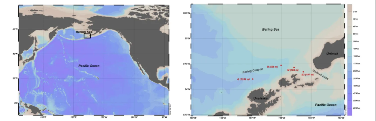
Samples were collected during MR17-04 cruise Leg2 on JAMSTEC R/V Mirai from 5 to 21 August 2017 in the southeastern Bering Sea. Given the scarce information about foraminiferal faunas in this area, three stations (G-1536 m, B-536 m, and M-103 m) along the Bering canyon were chosen to cover a wide range of environmental conditions: station G at middle bathyal depth, station B at upper bathyal depth and station M at the canyon head (Figure 1). One station (E2-197 m; Figure 1) in the Unimak pass depression was also selected since bottom topography suggested potential organic matter accumulation. The bottom water oxygen concentrations at stations E2 and M were high (>218 µmol/L), although they decreased with increasing water depths along the canyon, resulting hypoxic conditions at upper bathyal station B (24 µmol/L) and at the middle bathyal station G (28µmol/L, Figure 2). The exact positions of all stations were determined based on the Multi-narrow Beam Echo Sounding system (SeaBeam3012, Wärtsilä ELAC Nautik, Finland) bottom-topography surveys and Sub-Bottom Profiling (Bathy-2010, SyQwest, United States) surface sediment surveys to obtain stratified sediments (Table 1).
At all 4 stations, surface sediment cores (7.4 cm inner diameter and typically longer than 10 cm) were collected using a multiple corer (Barnett et al., 1984). Cores dedicated to sediment analyses (TOC, granulometry, pore-water nutrients and pheopigments) were sliced every cm down to 5 cm (with the exception of the core used for oxygen microprofiling which was left intact) while cores dedicated to foraminiferal fauna analysis were sliced down to 3 cm with a 0.5-cm resolution. Due to limited sediment material, at each station, one core was divided into 2 equal portions, with one half dedicated to foraminiferal analyses and the other half was preserved for prokaryotes cell count.
At stations B, G, and E2, we collected additional sediment cores for the isolation of living foraminiferal specimens to examine intracellular nitrate concentrations of foraminifera and their denitrification activity.
Water Column Conditions
Water column properties were analyzed through a CTD-sensor (SBE9plus, Sea-Bird Electronics, United States) profiling to measure temperature, salinity, dissolved oxygen, fluorescence, and turbidity along the canyon axis. The CTD-sensor collected data from the water column surface down to 5 to 10 m above seafloor.
Sediment Characteristics
Total Organic Carbon (TOC) and Total Nitrogen (TN) Concentrations
The sediment samples used for TOC and TN concentrations were freeze-dried, pulverized, and then weighed into pre-cleaned silver capsules. The samples were decalcified with 2 M HCl followed by drying on a hot plate (60◦
C). Silver capsules containing decalcified dry samples were sealed into pre-cleaned tin capsules prior to analysis. TOC and TN content were analyzed using an elemental analyzer (Flash EA 1112, Thermo Fisher Scientific, United States), and C/N ratio (weight/weight) was determined with the measured TOC and TN values.
Chloro- and Pheopigments Concentration
Total chloro- and pheopigments concentration in 0–1 cm depth interval of the sediment was quantified by summing up Chlorophyll a, Pheophytin a, Cyclopheophorbide a enol, and Pyrophenophytin concentrations. Pigments were extracted from dried sediment samples by sonication in acetone. The supernatant was dried up and dissolved in N,N-dimethylformamide (Naeher et al., 2016). Concentrations of each pigments were measured by Agilent 1100 series HPLC attached with an Agilent Eclipse XDB-C18 column (250 mm × 4.6 mm; 5 µm) connected with an Agilent Eclipse XDB-C18 guard column (12.5 mm × 4.6 mm; 5 µm). Pigments were eluted by two eluents: acetonitrile/pyridine (100:0.5; v:v) and ethyl acetate/pyridine (100:0.5; v:v).
Chloro- and pheopigment concentrations are presented as absolute value when expressed per mass of sediment and as relative value when normalized by TOC mass at a given station.
Pore-Water Oxygen Distribution
Dissolved-oxygen concentration in sediment pore water was measured in a temperature-controlled room (at 6◦
C) in intact cores as soon as cores were brought on deck. Oxygen concentration was determined using 50-µm tip-diameter oxygen microsensor (Unisense, Denmark;Revsbech, 1989) for samples at stations G and B and a sensor enclosed in a 1 mm diameter needle for samples at stations M and E2 due to the large quantity of gravel and shells in the sediment in these stations. Sensors were 2-points calibrated using an oxygen-saturated seawater at 6◦
C and an anoxic solution (prepared using 20 g of sodium ascorbate per liter of 0.1 mol/L NaOH solution). Vertical microprofiling was performed by placing the microsensor on a motor-controlled micromanipulator (Unisense, Denmark).
Porewater Nutrient Concentrations
Porewater samples were extracted from sliced sediments by centrifuging and were analyzed for nutrient concentrations (Nomaki et al., 2016;Amaro et al., 2019). Approximately 20 mL of overlying water was gently removed using a tube and then passed through a 0.45-µm membrane filter. Approximately 40 mL per 1 cm depth of sediment samples were put into 50 mL conical tube and were centrifuged at 2600 ×g for 5 or 10 min. Supernatant was gently suctioned with a 20 ml plastic syringe and filtered through a 0.45-µm membrane filter. Due to low water content, it was not
FIGURE 1 | Bathymetric map of the northern Pacific and southeastern Bering with the location of the sampling stations (red circles) along the Bering Canyon and in the Unimak pass.
FIGURE 2 | Water column profiles of temperature, salinity, oxygen, fluorescence, and turbidity. Note that the depth and distance scales are stretched. Stations sampled for benthic foraminiferal analysis are identified with black triangles.
possible to analyze nutrient content in layers deeper than 1 and 2 cm at stations M and E2, respectively.
Nutrient concentrations were measured with a continuous-flow analyzer (BL-Tech QUAATRO 2-HR system;Nomaki et al., 2016). The precision of the nitrate, nitrite, and ammonium
measurements, based on duplicate measurements, was ±0.17, ±0.16, and ±0.38%, respectively. When a nutrient concentration exceeded the calibration range, the filtrated porewater was diluted with nutrient-depleted seawater up to 20 times, and the concentrations were measured again to reduce the concentration
TABLE 1 | Water depth, sampling date, coordinates and number of sediment cores dedicated to faunal analysis at all sampling stations.
Site location Station Water depth (m) Sampling Date Latitude Longitude Foraminifera analysis (number of cores)
Bering Canyon G 1536 15-Aug-17 54-11.76N 166-58.34W 2
Bering Canyon B 536 7-Aug-17 54-28.42N 166-01.44W 2
Bering Canyon M 103 10-Aug-17 54-25.87N 165-35.21W 2
Unimak pass E2 197 12-Aug-17 54-20.62N 165-16.52W 3
within the calibration range. The original concentrations were calculated by considering the dilution ratios and the nutrient concentrations of the nutrient-depleted seawater.
Oxygen and Nitrogen Fluxes Estimation
Oxygen and NO3−+NO2− fluxes (J; in µmol/m2/day) at the
sediment-water interface were determined using Fick’s first law of diffusion as follow:
J = −8Ds × dC/dz
With8 being the sediment porosity estimated from the median grain size D50 at each station followingSchulz and Zabel (2006)
(such as porosity is about 0.6 in the bathyal stations G and B and 0.5 in the shallow stations M and E2). The molecular diffusion coefficient in the sedimentDs was calculated as:
Ds = D/(1 − log(82))
followingBoudreau (1997)withD being the molecular diffusion coefficient in water at 34 PSU and 6◦
C (1.4 and 1.1 10−5
cm2/s
for oxygen and NO3−+NO2−, respectively). dC/dz is the
concentration gradient (in µmol/cm4) with depth in the zone where dissolved oxygen and NO3−+NO2− decrease linearly.
Oxygen and NO3−+NO2− fluxes are, respectively, named
diffusive oxygen uptake (DOU) and NO3−+NO2− reduction
rates in this manuscript.
Use of Complementary Unpublished Data
For the Canonical Correspondent Analysis (CCA, see section “Data Analysis”), we used unpublished median grain size (D50) and prokaryotes cell number data from the 0–1 cm depth interval of the sediment. The grain-size were analyzed using a laser granulometer (SALD-2100, Shimadzu Corporation, Japan) according to the method described in Seike et al. (2018). Prokaryote cell numbers were determined by epifluorescence microscopy after extraction of cells from the sediment using pyrophosphate (final concentration, 5 mmol/L), sonication, and staining with SYBR Green I (Danovaro, 2009).
Foraminiferal Fauna Analysis
Two to three cores per station (Table 1) were sliced every 0.5 cm down to 3 cm depth. Each sediment layer was mixed with filtered seawater, dimethyl sulfoxide (DMSO) and 1 µmol/L final concentration of CellHunt Green CMFDA (5-chloromethylfluorescein diacetate, Setareh Biotech) hereby abbreviated CTG (Bernhard et al., 2006). The samples were then stored in a dark cold room at 6◦
C for 24 h, to permit the hydrolysis of the CTG compound in the live foraminiferal
cells. After this 24-hour incubation period, samples were fixed with a solution of 4% formaldehyde, pH-buffered with sodium tetraborate to prevent the leaking of the fluorogenic compound out of the foraminiferal cell. CTG allows to differentiate living (fluorescent) specimens from dead ones and is well-adapted to studies in low-oxygen environments since it allows to discriminate metabolically-active individuals (Pucci et al., 2009;
Richirt et al., 2020).
Back in the laboratory, metazoan meiofauna was removed from the sediment samples by density separation (Giere, 2009). Sediment was centrifuged at 3000 rpm for 10 min 3 consecutive times in a 1.17 g/cm3 Ludox R
density medium. Supernatant containing metazoans was removed, and sediment residues containing foraminifera were rinsed with 125 and 500µm sieves to facilitate foraminiferal sorting (Langlet et al., 2013, 2014).
Living foraminifera were sorted out of the sediment under an epifluorescence stereomicroscope (Olympus SZX16 with a fluorescent light source Olympus KL1600pE −300) at 492 nm excitation and 517 nm emission wavelength. Individuals with a bright fluorescence were picked with a brush and placed in cardboard plummer cell microslides to proceed to taxonomic recognition and counting. Individuals counts (available in
Supplementary Table S1) were normalized by the core section area (43 cm2for entire core and 21.5 cm2for half-split core) to calculate abundances at each station. A total of 41 species were identified from 4 stations and named after the World Register of Marine Species database (Horton et al., 2020). To simplify the discussion, we selected only the major species distribution (i.e., 13 species, which each represented more than 5% of the total fauna in at least one station). SEM images of the major species can be found in Supplementary Figure S1.
Species richness (S) was calculated as the number of living species in each sample and used to estimate Shannon index evenness (E) as follow:
E =6(pi×log2(pi))/log2(S)
withpi, the relative abundance of each species in the sample.
Cellular Nutrient Content and
Denitrification Rate Measurement
On board, foraminifera were picked in a chilled-petri dish under binocular microscope. Only specimens leaving a displacement track on a thin layer of sediment and confirmed active were selected and rinsed three times in nitrate-free artificial seawater (ASW; prepared from 35 g of Red Sea Salt per liter of Milli-Q ultrapure water). Individual size (maximum and minimum diameter) was measured using a graduated microscale placed
on the stereomicroscope eye piece to determine their biovolume (following Hannah et al., 1994; Geslin et al., 2011) and 2 to 10 individuals of the same species were pooled together to test denitrification activity. The pooled specimens were transferred to a microtube containing anoxic and nitrate free ASW to perform denitrification measurements. Since individuals were selected based on their occurrence in natural sediment and specimen’s vitality it was not possible to analyze all the main species.
Nitrate respiration rates were then determined based on Fick’s first law of diffusion from steady-state N2O profiles
measured with a N2O micro electrodes (Andersen et al., 2001)
after acetylene inhibition of N2O reduction (Smith et al., 1978;
Risgaard-Petersen et al., 2006;Høgslund et al., 2008).
Foraminifera were retrieved after the denitrification measurements and placed in centrifugation microtubes and frozen at −80◦
C to break the foraminiferal cell and conserve the samples until further nutrient content analysis.
Cellular nutrient measurement method fromNomaki et al. (2015) was modified to allow for simultaneous quantification of the ammonium ion and the sum of nitrate and nitrite. Nutrients extraction from the foraminiferal cells was achieved by freezing at −80◦
C, and the frozen cells were then dissolved in 500µL of Milli-Q water and homogenized in the microtube using a plastic pestle. Dissolved nutrients were separated into two aliquots to quantify the ammonium and sum of nitrate and nitrite (NO3− + NO2−) concentrations. NO3− + NO2− was
determined by the vanadium (III) chloride reduction method adapted from Doane and Horwáth (2003)where 160µL of the aliquot was mixed with 20µL of nitrate reductant (8 g of VCl3per
liter of 0.6 mol/L HCl) and 20µL of color reagent (prepared from 2 g sulfanilamine and 100 mg N-(1-naphthyl)ethylenediamine dihydrochloride per liter of 0.6 mol/L HCl) and heated at 60◦
C for 2 h. Calibration was performed using 0.1 to 50 µmol/L NO3−+NO2− standards prepared with KNO3 and Milli-Q
water. The NO3−+NO2− concentration was determined from
the absorbance at a wavelength of 540 nm with a UV-VIS spectrophotometer (UV-1800, Shimadzu corp.). Ammonium ion (NH4+) concentration was determined by mixing 200µL of the
aliquot with 8µL of phenol nitroprusside reagent (made from 20 mL of phenol and 0.125 g of nitroprusside per liter of Milli-Q water) and 20 µL of sodium hypochloride reagent (made from 10 mL of 5% Cl sodium hypochloride, 8 g of NaOH and 160 g of sodium citrate per liter of Milli-Q water) and heated at 30◦
C for at least 30 min. Calibration was performed using 0.1 to 50µmol/L NH4+standards prepared with NH4Cl and Milli-Q
water. Absorbance of the solutions were measured at 630 nm to determine NH4+concentration in the aliquots.
Nutrient concentrations in the aliquots were used to calculate individual nutrient content (in pmol per individual) and normalized by the biovolume to estimate intracellular nutrient concentrations.
Further measurement of intracellular nitrate concentrations and denitrification rate were performed in the laboratory on land 3 and 8 months after the sediment collection, to explore potentials to store nitrate and denitrification among different foraminiferal species (Supplementary Table S2). Living foraminifera were isolated from the sediment stored at 6◦
C in the same manner
as the measurements on board. Because we cannot exclude possible artifact on the exact concentration of intracellular nitrate and denitrification rate, we only use onboard results for the quantification of foraminiferal roles in N cycles.
Data Analysis
Water column profiles maps were visualized on Ocean Data View using weighted-average gridding (Schlitzer, 2002). Differences in foraminiferal abundances, species richness and diversity in the top cm of the four sampled stations were tested using analysis of variance (Chambers and Hastie, 1992). Canonical Correspondent Analysis (CCA) was used to identify the link between 15 environmental parameters (station water depth, bottom water turbidity, bottom water oxygen concentration, oxygen penetration depth, diffusive oxygen uptake, sum of nitrate and nitrate concentration in overlaying water, sum of nitrate and nitrite concentration in the top cm porewater, sum of nitrate and nitrate reduction rates, TOC in the top cm of the sediment, C:N ratio of the top cm of the sediment, number of prokaryotes cells in the top cm, pheopigments per gram of sediment in the top cm, pheopigments per mg of TOC in the top cm, chlorophylla per gram of sediment in the top cm, and median grain size in the top cm) and the foraminiferal distribution in the 4 stations. Untransformed counts in the 0–1 cm depth interval of the 13 major species were chosen to describe foraminiferal community. Analyses were performed on R v. 3.6.2 (R Core Team, 2019) using the ade4 package (Thioulouse et al., 1997).
RESULTS
Environmental Setting
Water Column
CTD data showed that water temperature ranged from 2◦
C at the bottom of the station G to 10◦
C at the sea surface of the shallowest station M with a strong thermocline near 100 m water depth (Figure 2). Lower salinities were measured at the sea surface in the Unimak pass (32.5 PSU at station E2) and higher values observed in the bottom-waters of station G (34.5 PSU).
Sea-surface oxygen concentration was similar at all stations with values ranging from 274 to 304µmol/L (Figure 2). Highest fluorescence (3.8µg/L) was observed at the surface water above the shallowest station M, while they were 2.2, 1.8, and 2.7µg/L at stations G, B, and E2, respectively. Turbidity values ranged from 0.32 to 0.40 at stations G, B, and M, and 0.19 at the surface of E2 (Figure 2).
Bottom-water in the upper bathyal and middle bathyal stations were characterized by low oxygen concentrations (28 and 24µmol/L at stations G and B, respectively) while oxygen was close to saturation at the shallowest stations M and E2 (218 and 224µmol/L respectively; Figure 2). Bottom-water turbidity was 0.43 and 0.40 at stations G and B, respectively and reached 0.07 and 0.16 at stations M and E2, respectively (Figure 2).
Sediment Geochemistry
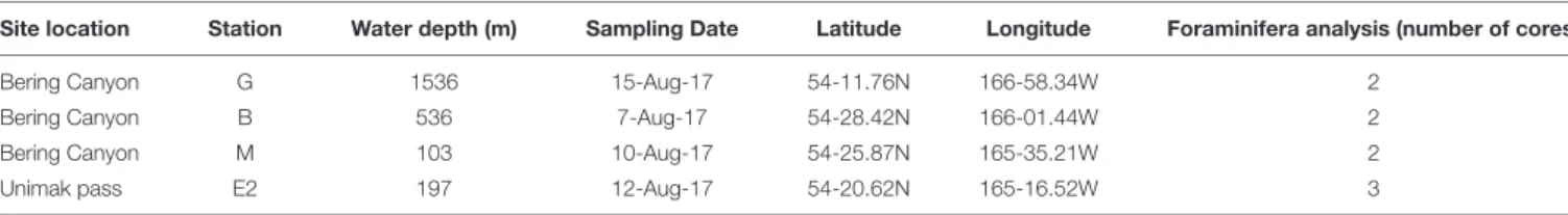
Total organic carbon (TOC) concentrations in sediments were higher in the bathyal stations G and B (up to 39.8 and 40.6 mg/g,
respectively) than in the shallow stations M and E2 (up to 1.5 and 2.5 mg/g, respectively). At the upper bathyal station B, TOC showed a strong decrease between the 0–1 and 1–2 cm depth intervals while at middle bathyal station G, TOC remains constant between 0 and 5 cm (Figure 3). At the shallowest stations, TOC was relatively stable with depth ranging from 0.9 to 2.2 and 1.6 to 2.5 mg/g, respectively at station M and E2. Organic matter C/N in the top cm ranged from 6.9 to 8.1 with increasing values from east to west along the Bering Canyon (Table 2). High pheopigment concentrations in the top cm were measured in the high TOC stations (1.63 and 2.37 nmol/g at stations G and B, respectively) while coarse-sand stations showed low pheopigments concentrations (0.03 and 0.34 nmol/g at stations M and E2, respectively). When normalized by the quantity of TOC, relative pheopigments concentration in total organic carbon was larger at station E2 (0.14 nmol/mgTOC) than in other stations (ranging from 0.02 to 0.06 at stations G, B, and M).
Oxygen microprofiles at stations G, B, and M showed gradual decrease in dissolved oxygen concentration with increasing sediment depth, and the oxygen penetration depths were 5 mm at bathyal stations G and B and 17 mm at station M. Station E2 showed stepwise decrease in oxygen concentration with depth with high consumption in the 0–5 and 15–20 mm depth intervals.
At this station, the measured oxygen penetration depth was about 22 mm. Sediment oxygen consumption as estimated from diffusive oxygen uptake (DOU) was maximal at station B (about 2000 µmol/m2/day), minimal at stations G and M (330 and 307µmol/m2/day, respectively), and intermediate at station E2 (752µmol/m2/day; Table 2).
Pore-water nutrient distribution also showed contrasted conditions between bathyal and shallow stations. At the hypoxic stations G and B, the sum of nitrate and nitrite NO3−+NO2−
concentrations was larger in the overlaying water than in the pore-water (Figure 3) suggesting nitrate and nitrite reduction at the sediment-water interface. Station B presented lower NO3−+NO2− concentrations in the sediment than at station
G (ranging from 8.8 to 4.8 µmol/L at station B and from 34.4 to 19.6 µmol/L at station G in the top 2 cm) which resulted in more intense NO3−+NO2− reduction rates estimates at
station B (Table 2). At the well-oxygenated stations M and E2, NO3−+NO2− concentration in the overlaying water was lower
than in the pore-water of the top cm. Maximal NO3−+NO2−
reduction was estimated at the sediment-water interface of station B (99 µmol/m2/day), stations G and E2 presented intermediate values (33 and 41 µmol/m2/day, respectively, estimated in the overlaying water −2 cm depth interval at station
0 100 200 0 10 20 30 40 50 Station G (1536 m) 50 40 30 20 10 0 − 10 Depth (mm) O2concentration (μmol/L)
[NO3−+ NO2−] concentration (μmol/L)
TOC (mg/g) 0 100 200 0 10 20 30 40 50 Station B (536 m) 0 100 200 0 10 20 30 40 50 Station M (103 m) 0 100 200 0 10 20 30 40 50 Station E2 (197 m)
FIGURE 3 | Dissolved oxygen (black open circles) and sum of nitrate and nitrite (NO3-+ NO2-); red open circles with red dotted line) concentration in overlaying
T ABLE 2 | Organic matter C/N ratio, median grain size (D50) (K. Seike, unpublished data), pheopigment concentration (absolute: expr essed per gram of sediment and relative: expr essed per mg of TOC) and chlor ophyll a concentration in the top cm of the sediment with dif fusive oxygen uptake (DOU) and NO 3 −+ NO 2 − reduction rate, and pr okaryotes cell numbers (H. Nomaki, unpublished data) at all stations. Station W ater depth C/N [0-1 cm] D50 [0-1 cm] Pheopigments [absolute] Pheopigments [r elative] Chlor ophyll a [0-1 cm] DOU NO 3 + NO 2 reduction rate Pr okaryotes cells (m) (wt/wt) (mm) (nmol/g) (nmol/mg TOC) (nmol/g) (mmol/m 2/day) (mmol/m 2/day) (10 − 8cell/mL sed) G 1536 8.1 0.02 1.63 0.04 0.37 330 33 2.0 B 536 7.5 0.03 2.37 0.06 0.14 1994 99 2.0 M 103 7.5 0.49 0.03 0.02 0.00 752 12 0.3 E2 197 6.9 1.06 0.34 0.14 0.02 307 41 0.7
G and in the 0–2 cm depth interval at station E2), and was minimal at station M (12µmol/m2/day; Table 2, estimated in
the 1–7 cm depth interval). Changes in nitrate + nitrite in sediment pore water were mainly driven by changes in nitrate concentration since they represented over 90% of NO3−+NO2−
at all stations and all depths (with the exception of nitrate-poor station B, at 2–5 cm depth, where NO3−contributed from 60 to
80% to the total nitrate-nitrite concentrations).
Faunal Distribution
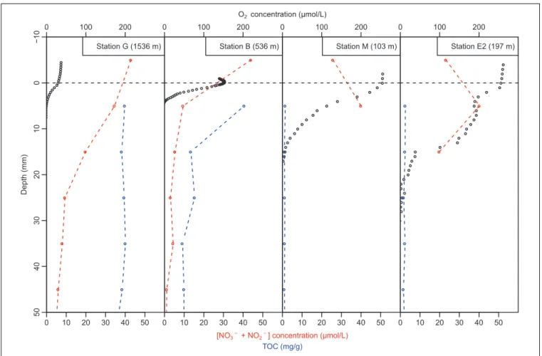
Total foraminiferal abundance in the top 3 cm of the sediments ranged from 179 to 909 ind./50cm2 (Figure 4). At all stations,
maximum abundances were observed in the top cm and tended to decrease with depth in the sediments particularly at stations B and E2 (Figure 4). Abundances in 0–1 cm depth intervals ranged from 121 ind./50cm2at station M to 765 ind./50cm2 at station E2 and did not show any significant differences between stations (F = 2.3, df = 3 and 5; p = 0.2). Species richness showed significant differences between stations (F = 8.2, df = 3 and 5, p = 0.02) such as the number of species was larger at station E2 (from 22 to 30 species per core) than station G, B, and M (from 11 to 22 species per core). Shannon evenness, however, ranged from 0.73 to 0.85 and did not show any significant differences between stations (F = 3.8, df = 3 and 5, p = 0.09).
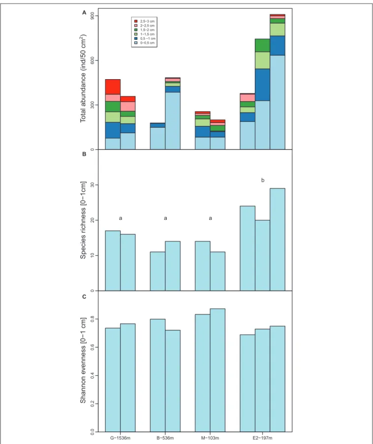
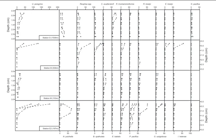
Foraminiferal communities at the middle bathyal station G (1536 m) were dominated by Uvigerina peregrina which was present mainly in the top 2 cm (representing 32 and 19% of the total population in the 0–1 and 1–2 cm depth intervals, respectively),Nonionella pulchella which was present both at the surface and subsurface in the sediments (over 12, 24, and 36% in the 0–1, 1–2, and 2–3 cm depth intervals, respectively),Elphidium batialis at the sediment-water interface (representing 19, 8, and 2% of the foraminiferal community in the 0–1, 1–2 and 2–3 cm depth intervals) andGlobobulimina pacifica in deeper layers (over 8% of the total foraminiferal community in the 2–3 cm depth interval; Figure 5).
Upper bathyal station B (536 m) showed a sharp decrease in abundances with depth for most species (Figure 5), foraminiferal fauna in the uppermost centimeter was dominated byUvigerina peregrina, Reophax spp., Bolivina spathulata, Islandiella helenae, Recurvoides trochamminiformis, and Eggerella bradyi (29, 19, 16, 10, 8, and 6% of the 0–1 cm fauna, respectively) while subsurface samples (1–2 and 2–3 cm) were mainly dominated by the agglutinated speciesReophax spp., Recurvoides trochamminiformis, and Eggerella bradyi (Figure 5).
At the shallow station M (103 m), surface (0–1 cm) fauna was dominated by Uvigerina peregrina, Cibicidoides wuellerstorfi, Recurvoides trochamminiformis, Recurvoidella bradyi, Globocassidulina subglobosa, Portatrochammina pacifica, andBolivina spathulata (respectively, 26, 15, 10, 10, 8, 8, and 6% in the 0–1 cm interval). These species also dominated subsurface layers (over 9% for each species of the total fauna) except for Bolivina spathulata which represent less than 1% of the living foraminifera below 1 cm (Figure 5).
In the Unimak pass depression, at the station E2 (197 m), the abundant surface fauna was mainly composed of Uvigerina peregrina, Portatrochammina pacifica, Recurvoides
0 3 00 600 900 2,5−3 cm 2−2,5 cm 1,5−2 cm 1−1,5 cm 0,5 −1 cm 0−0,5 cm To
tal abundance (ind/50 cm
2) 01 0 2 0 3 0 a a a b Species r ichness [0−1 cm] G−1536m B−536m M−103m E2−197m 0.0 0 .2 0.4 0 .6 0.8 Shannon e venness [0−1 cm] A B C
FIGURE 4 | (A) Total foraminiferal abundances combined from each sediment layer (light blue: 0–0.5 cm, dark blue: 0.5–1 cm, light green: 1–1.5 cm, dark green: 1.5–2 cm, light red: 2–2.5 cm and dark red: 2.5–3 cm). (B) Species richness in the top centimeter at all stations. (C) Shannon evenness in the top centimeter at all stations. Letters a and b indicate the stations with significantly different species richness (following analysis of variance). Note that no data are available in the 2–3 cm depth intervals in one replicate core at station B and E2.
0 50 100 150 200 250 U. peregrina 3.0 2.5 2.0 1.5 1.0 0.5 0.0 Depth (cm) Station G (1536m) Station B (536m) 3.0 2.5 2.0 1.5 1.0 0.5 0.0 Depth (cm) Station M (103m) Station E2 (197m) 0 50 100 N. pulchella 0 50 100 Reophax spp 0 50 B. spathulata 0 50 C. wuellerstorfi 0 50 E. batialis 0 50 R. trochamminiformis 0 50 P. pacifica 0 50 100 R. bradyi 0 50 G. subglobosa 0 50 E. bradyi 0 50 100 I. helenae 0 50 G. pacifica 3.0 2.5 2.0 1.5 1.0 0.5 0.0 Depth (cm) Depth (cm) 3.0 2.5 2.0 1.5 1.0 0.5 0.0
FIGURE 5 | Vertical distribution of the 13 major species at the four sample locations. Abundances of each species are presented in number of individuals per 50 cm2. Note that 2–3 cm samples were not examined in one replicate core of stations B and E2.
trochamminiformis, and Nonionella pulchella (over 31, 9, 7, and 7% of the fauna, respectively, Figure 5). Portatrochammina pacifica and Nonionella pulchella were also observed in large numbers below 1 cm (each representing more than 15% of the foraminiferal community).
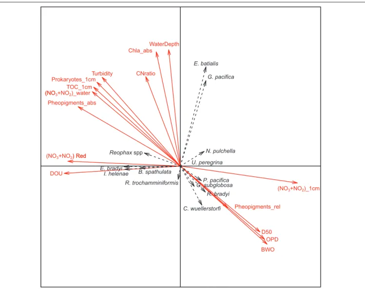
The two first axes of the canonical correspondence analysis (CCA) represented 27 and 23% of the total dataset inertia. The first axis showed a negative correlation of NO3−+NO2−
concentration in the top cm of the sediment with both NO3−+NO2− reduction rate and diffusive oxygen uptake.
These 3 parameters were poorly correlated with water depth, chlorophyll a concentration in the top cm and C:N ratio which contributed strongly to the second axis (Figure 6). Results also showed that prokaryote density, TOC, and absolute pheopigment concentration in the top cm of the sediment, bottom-water turbidity and NO3−+NO2− concentration were
negatively correlated to relative pheopigment concentration, oxygen penetration depth, median grain size, and bottom-water oxygen concentration (Figure 6).
In the CCA,Reophax spp., Eggerella bradyi, Islandiella helenae, and Bolivina spathulata are all grouping on axis 1, therefore showing high affinity to intense sedimentary NO3−+NO2−
reduction and oxygen consumption rates (Figure 6).Cibicidoides wuellerstorfi, Globocassidulina subglobosa, Portatrochammina
pacifica, and Recurvoidella bradyi were grouping in the same direction as pheopigments, bottom-water oxygen, and oxygen penetration depth.Elphidium batialis and Globobulimina pacifica were the only species with a strong loading on CCA axis 2 and were associated with water depths. Nonionella pulchella and Recurvoides trochamminiformis seemed to be negatively correlated with each other and appeared orthogonal to most of the environmental variables (Figure 6). Finally, Uvigerina peregrina presented low loadings on both CCA axis 1 and axis 2.
Cellular Nutrients Accumulation and
Denitrification
The five tested foraminiferal species had nutrients in their cells with nitrate quantities ranging from 16 to 17600 pmol/ind. and ammonium ranging from 21 to 106 pmol/ind (Table 3 and Supplementary Table S2). Larger nitrate concentrations were detected inBolivinella pseudopunctata (148 mmol/L) and Globobulimina pacifica (648 mmol/L). Within the five tested species, onlyG. pacifica, B. spathulata and one set of Nonionella pulchella could reduce nitrate through denitrification with denitrification rates ranging from 6 to 711 pmol/ind/day. In addition, two unidentified Gromiids species showed nitrate quantities ranging from 282 to 452 pmol per cell with
BWO OPD TOC_1cm CNratio Prokaryotes_1cm DOU Chla_abs D50 Turbidity Pheopigments_abs Pheopigments_rel U. peregrina N. pulchella Reophax spp. B. spathulata C. wuellerstorfi E. batialis R. trochamminiformis P. pacifica R. bradyi G. subglobosa E. bradyi I. helenae G. pacifica (NO3+NO2)_1cm (NO3+NO2) Red
(NO3+NO2)_water
) Red (NO
WaterDepth
FIGURE 6 | Canonical correspondence analysis of foraminiferal counts in the 0–1 cm depth interval of the major species (black labels and dotted line arrows) and environmental data (bold red labels and arrows). Environmental variables are abbreviated as follow: DOU = diffusive oxygen uptake, (NO3+NO2) Red = sum of nitrate
and nitrate reduction rates, (NO3+NO2)_water = sum of nitrate and nitrate concentration in overlaying water, TOC_1 cm = total organic carbon in the top cm of the
sediment, Prokaryotes_1 cm = number of prokaryotes cells in the top cm, Turbidity = bottom water turbidity, CNratio = C:N ratio of the top cm of the sediment, WaterDepth = station water depth, (NO3+NO2)_1 cm = sum of nitrate and nitrite concentration in the top cm porewater, pheopigments_abs = pheopigments per
gram of sediment in the top cm, pheopigments_rel = pheopigments per mg of TOC in the top cm, Chla_abs = chlorophyll a per gram of sediment in the top cm, D50 = median grain size in the top cm, OPD = oxygen penetration depth, and BWO = bottom water oxygen concentration.
denitrification rates varying from 16 to 108 pmol/ind/day (Table 3 and Supplementary Table S2).
DISCUSSION
Foraminiferal Community Relationship
With Environmental Conditions
This study, like previous works (Reeburgh and Kipphut, 1986;
Roden, 1995), confirms the occurrence of hypoxic conditions in the bathyal Bering Sea stations B and G (∼500–1500 m) leading to low species richness and foraminiferal communities dominated by hypoxia-resistant species like in other permanent low-oxygen systems (Koho and Piña-Ochoa, 2012). However,
hypoxic conditions have limited effect on total foraminiferal abundances since more living foraminifera were found at the stations E2 and B than at stations G and M (Figure 4) likely because dissolved oxygen is not severely depleted enough to limit foraminiferal distribution. Higher organic matter availability at the bathyal silty stations G and B than at the shallow sandy stations M and E2 (as suggested by TOC, pheopigments, bottom-water turbidity and granulometry measurements) likely compensate the potentially-adverse effects of bottom-water hypoxia. Foraminiferal abundances at the sediment-water interface might rather be controlled by the availability of fresh organic matter as previously shown in other low-oxygen settings (Gustafsson and Nordberg, 1999; Langlet et al., 2013; Richirt et al., 2020). The organic matter measured in the sediment likely
T ABLE 3 | Foraminifera and Gr omiids nutrient intracellular accumulation and nitrate respiration for all tested species. Species Station W ater depth (m) Number (indiv .) Biovolume (10 6µ m 3) Session Intracellular NO 3 Intracellular NH 4 Quantity (pmol/indiv) Concentration (mmol/L) Denitrification rate (pmol/ind/day) Quantity (pmol/indiv) Concentration (mmol/L) Nonionella pulchella B 536 11 12 onboar d 31 3 0 21 2 Bolivina spathulata B 536 19 10 onboar d 154 15 11 63 6 Globobulimina pacifica B 536 5 23 onboar d 1928 82 711 106 5 Uvigerina peregrina B 536 10 18 onboar d 96 5 0 56 3 Uvigerina peregrina B 536 10 5 onboar d 92 19 0 42 9 Bolivinellina pseudopunctata B 536 11 1 onboar d 133 148 0 28 31 Globobulimina pacifica G 1535 4 27 onboar d 17602 648 45 70 3 Melonis affinis North Sea NA NA 14 Piña-Ochoa et al. , 2010 9 0.6 NA NA NA Pyrgo spp. Rhône Delta NA NA 47 Piña-Ochoa et al. , 2010 43 0.8 NA NA NA V alvulineria spp. OMZ Peru NA NA 19 Piña-Ochoa et al. , 2010 865 25 248 NA NA Chilostominella oolina Bay of Biscay NA NA 20 Piña-Ochoa et al. , 2010 1124 65 NA NA NA Each row corresponds to one replicate in which a set of a multiple numbers of individuals is tested. Intracellular nutrient concentration is derived from the measured intracellular nutrient quantity and the average biovolume. This table presents data from foraminifera extracted from the sediment onboard (in the week following sampling) as well as four species published in Piña-Ochoa et al. (2010 ) also found in the Bering Sea.
originated from the intense surface productivity (Sambrotto et al., 1984; Stabeno et al., 1999) linked to upwelling activity (Kelley et al., 1971;Fransson et al., 2006). In fact, productivity was so intense that the “Aleutian magic” phenomenon (a gathering of whales and thousands of sea birds feeding on krill, planktonic gastropods, and juvenile cods) was observed at the head of the canyon near station M during the cruise. Surprisingly, this high productivity has little impact on fresh organic matter deposit in the station M sediment probably because of a strong bottom current leading to coarse bottom sediments as reported in previous studies (Roden, 1995;Stabeno et al., 2016) and shown by bottom-water observations during our cruise (Y. Fujiwara, pers. comm.). Instead, the fresh labile organic matter produced at the sea surface seems to accumulate at station E2, situated in a depression in the Unimak pass as indicated by the high pheopigments quantity, leading to high foraminiferal abundances and species richness. The oligotrophic benthic conditions at station M limited foraminiferal density affecting especially Uvigerina peregrina which is otherwise strongly dominant at other stations, leading to relatively high diversity at this station. Overall, diversity indices calculated on southeastern Bering foraminiferal fauna are in the same order of magnitude as those reported from other North Pacific areas (Bubenshchikovaa et al., 2008; Venturelli et al., 2018) yet do not seem to be affected by low-oxygen concentration unlike previous reports in OMZ (Gooday et al., 2000; Caulle et al., 2014) or coastal hypoxic areas (Blackwelder et al., 1996; Filipsson and Nordberg, 2004;
Bouchet et al., 2012).
At all stations, foraminifera preferably colonized sediment layers where oxygen was available as predicted by the vertical microhabitat segregation vertical model byJorissen et al. (1995)
except for station G where a relatively large number of individuals are living below the oxygen penetration depth. At this station, TOC concentrations were also stable from 0 to 5 cm depth while at station B these three variables decreased with depth. This suggests that organic matter availability in the sediment column could influence foraminiferal vertical distribution as previously shown in other low-oxygen areas of the North Pacific (Fontanier et al., 2014). The difference in TOC vertical distribution at stations B and G could be due to the high oxygen fluxes calculated at station B which might be correlated to a strong nitrate consumption at the sediment-water interface. Although oxygen fluxes at this station might be overestimated due to oxygen contamination (as indicated by the oxygen concentration in the overlying water higher than 100µmol/L during profiling while CTD data showed 24 µmol/L O2 in the bottom-water), our
results suggest that organic matter mineralization could be more intense at station B than in all the other stations (Middelburg, 2019). The foraminiferal vertical distributions in the top 3 cm at stations G and B is likely mitigated by an organic matter, oxygen, and nitrate availability as shown in other hypoxic settings (Glud et al., 2009;Fontanier et al., 2014;Xu et al., 2017). They might also respond to low NO3−and NO2−availability in deeper
layers of the sediment at station B limiting the presence of deep-infaunal denitrifying species since nitrate’s absence can control these species growth and distribution (Xu et al., 2017;Glock et al., 2019). At stations M and E2 the high oxygen penetration depth
suggest that faunal distribution is rather structured by organic matter availability (Jorissen et al., 1995).
Species-Specific Distribution
Uvigerina peregrina was present at all the stations and show large abundances in the top layer of the sediments at stations G, B, and E2 (Figure 5). Such vertical distributional pattern is consistent with previous studies reporting surficial microhabitat (Jorissen, 1999). Low availability of fresh organic matter clearly limits this species abundances at station M, showing opportunistic response of the species to eutrophic conditions (Schmiedl et al., 2000;
Fontanier et al., 2003). This species is abundant in lower part of the Arabian Sea and Peruvian OMZ (Jannink et al., 1998;
Schumacher et al., 2007;Mallon et al., 2012) confirming its ability to withstand low-oxygen conditions. Our data also confirms that this species can accumulate nitrate (Piña-Ochoa et al., 2010) yet show that they cannot use it through denitrification (Table 3).
Portatrochammina pacifica was also observed at all the stations with higher abundances at station E2 (Figure 5). Such a broad range in water depth is rather common in trochamminids, frequently reported as continental shelves species (Murray, 2006) and also observed in deep-sea systems (Gooday, 1988) such as the Aleutian margin (Rathburn et al., 2009). In our samples, most living individuals were found in oxygenated layers of the sediment suggesting a shallow infaunal microhabitat. Information about this species’ habitat preferences is rather scarce in the literature, but other Portatrochammina species from Sulu Sea also live in a surface infaunal habitat (Szarek et al., 2007) while other species from the Polar Oceans have an intermediate infaunal microhabitat (Wollenburg and Mackensen, 1998;Sabbatini et al., 2004) and can survive anoxic conditions during a 1-month laboratory experiment (Bernhard, 1993) which could explain the presence of P. pacifica at the hypoxic stations G and B.
Bolivina spathulata was also present at all the stations with a peculiar vertical distribution pattern at the middle bathyal station G. This difference in vertical distribution could be linked to the organic matter availability in deep layers at station G. Indeed, this species is considered as indicator of high organic matter input (Jorissen, 1999;Fontanier et al., 2003;
Mojtahid et al., 2009) and can survive in low-oxygen conditions (Bernhard and Sen Gupta, 1999). Canonical correspondence analysis also suggests a negative correlation betweenB. spathulata and nitrate concentration in the 0–1 cm depth interval of the sediment, reflecting its presence in large number at the high nitrate consumption rate at station B. This species can use nitrate through denitrification and might therefore play an important role in a Bering Sea nitrogen cycle like other Bolivinds in the Northern and Eastern Pacific (Glud et al., 2009;
Glock et al., 2019).
Globocassidulina subglobosa and Recurvoides trochamminiformis occurred in the sediment surface layers of all the stations except station G. The former is common in the North Pacific within a wide depth range of habitats, from the 4000-m abyss (Enge et al., 2012) to bays at a depth of 50 m off California (Walton, 1955) and was shown to selectively feed on
phytodetritus (Suhr et al., 2003). Its absence at the chlorophyll-a-rich station G is surprising and might be due to competition with Elphidium batialis which occupies this microhabitat in station G. Little is known about R. trochamminiformis ecological preferences. It has been reported near 200 m depth in upper bathyal northern Bering Sea (Anderson, 1963), in the northeastern Atlantic Outer Continental Shelf (Murray, 2003), and in the Rhone delta as a surface infaunal species (Mojtahid et al., 2010). OtherRecurvoides species were also observed at the sediment-water interface in high-latitude environments (Hunt and Corliss, 1993) and abyssal East Pacific (Ricketts et al., 2009). Our results confirm these two species show surface infaunal microhabitats and suggest that their distribution could be limited by bottom-water hypoxia.
Cibicidoides wuellerstorfi and Recurvoidella bradyi were observed at the shallow stations M and E2 essentially in the top 1.5 cm of the sediments. This is especially surprising for C. wuellerstorfi which is broadly acknowledged as an epifaunal species (Lutze and Thiel, 1989;Linke and Lutze, 1993;Rathburn and Corliss, 1994; Rathburn et al., 2009; Burkett et al., 2016). Their presence relatively deep in the sediment could be explained by the high oxygen penetration depth and the high sand content which could allow to extend this specie’s habitat or by important sediment mixing that would burry these species. The sediment mixing hypothesis is supported by video survey showing intense bottom-water currents at stations M and E2 (Y. Fujiwara, pers. comm.) and reverse14C dating values in surface sediment at the same stations (K. Seike, pers. comm.) and was demonstrated to affect foraminiferal vertical distribution (Maire et al., 2016).
Reophax spp., Eggerella bradyi, and Islandiella helenae were found almost exclusively in the top 0.5 cm of station B (except forI. helenae which also show low abundances at the sediment– water interface at station E2) and should hence be considered as surface infaunal species. Station B is characterized by low nitrate concentration in the 0–1 cm sediment layer, these three species therefore appear to be negatively correlated to sedimentary nitrate concentration and could likely contribute to nitrate reduction. Reophax species are very common in the edge of the Indian margin OMZ (Gooday et al., 2000; Caulle et al., 2014) confirming that this genus can live under hypoxic conditions. In coastal environments,Eggerella and Eggerelloides species are also known to withstand anoxic conditions although these species rather occupy intermediate to deep infaunal microhabitats (Langlet et al., 2014; Cesbron et al., 2016). Finally, Islandiella helenae vertical distribution seems to be consistent with previous reports of this genus microhabitat in the Okhotsk Sea (Bubenshchikovaa et al., 2008) and other Arctic environments (Hunt and Corliss, 1993).
Elphidium batialis and Globobulimina pacifica were found almost exclusively at the deepest station G. The former is common in deep hypoxic North Pacific sediments (Usami et al., 2017) where it is conversely reported as a surface infaunal species (Bubenshchikovaa et al., 2008; Fontanier et al., 2014). This contrasts with G. pacifica which is thriving below 2 cm and is commonly known as a deep infaunal species (Jorissen, 1999) with abundances that can reach over 90 individuals/50 cm2
Species of the genus Globobulimina are recognized as being resistant to anoxic conditions (Koho et al., 2011) and consistently exhibit high denitrification rates (Risgaard-Petersen et al., 2006;
Piña-Ochoa et al., 2010).
Nonionella pulchella was present at stations G and E2 where it was observed in all the depth layers from 0 to 2 cm. In the literature, little is known about this species ecology and habitat preferences. Some studies report it at depths between 100 and 300 m in the Gulf of Alaska (Quinterno and Park, 1990) and around the same water depth in the Northwest Pacific (Asano, 1960). Our results suggest that this species could have an intermediate infaunal microhabitat similarly, from other Nonion-like species (Jorissen, 1999;Fontanier et al., 2002). Some of these species can use nitrate through denitrification ( Risgaard-Petersen et al., 2006;Høgslund et al., 2008;Piña-Ochoa et al., 2010;Glock et al., 2019) which we confirmed for only 1 set of specimens out of 6 forN. pulchella in the Bering Sea. If this species were in fact capable of denitrification, its absence at station B might therefore be explained by a strong competition for nitrate reduction at this station.
Role of Foraminifera in the Bering Sea
Benthic Ecosystem
In the Bering Sea, 9 of the total 43 species identified can accumulate nitrate in their cells. These 9 species accounted for 38 up to 60% of the foraminiferal abundances and are especially important at stations G and M (Table 4). Considering each species nitrate content (measured in freshly sampled individuals onboard) and abundance, the total foraminiferal nitrate content in the top 3 cm ranges from 0.2 to 4.1 µmol per liter of pore water. Intracellular nitrate content therefore contributes from 0.5 to 19.4% of the total nitrate pore water concentration in the Bering Sea while it can reach up to 20% in the Gullmar Fjord (Risgaard-Petersen et al., 2006) and 80% in the Sagami Bay (Glud et al., 2009). Larger contribution is estimated at the bathyal stations G and B likely due to their low pore-water concentrations (Figure 3).
Within the five species tested in this study, onlyGlobobulimina pacifica, Bolivina spathulata and Nonionella pulchella can reduce nitrate through denitrification (Table 3 and Supplementary
Table S2).Valvulineria spp. from the Peru OMZ can also perform denitrification (Piña-Ochoa et al., 2010) and occurred in low abundances at stations G, B and M (no more than 4 ind./50 cm2).
Since we did not find any actively moving individuals in the fresh sediment it was not possible to test the other major species for their denitrification capacities. Denitrification rates measured in G. pacifica in the Bering Sea are in the same order of magnitude as those reported in other environments for the same genus (Risgaard-Petersen et al., 2006; Piña-Ochoa et al., 2010). The four denitrifying species combined represented from 7 to 34% of the total foraminiferal fauna. In spite of these limitations, total foraminiferal nitrate reduction rates (obtained from combining denitrifying species abundance with their denitrification rates) reached up to 2 µmol/m2/day at station G representing from
0.2% at station M to 6% at station G of the total NO3−+NO2−
reduction rates. Nitrate and nitrite reduction in the sediment can TABLE
4 | Part of the total fauna accumulating nitrate, total foraminiferal nitrate content and its contribution to sediment nitrate content, foraminiferal denitrification, and its contribution to total nitrate reduction at all stations. Station Nitrate accumulating ind. (% specimens) Sedimentary nitrate content [0–3 cm] Denitrifying ind. (% specimens) Sediment nitrate reduction T otal foraminiferal NO 3 + NO 2 (umol/L) Por e water NO 3 + NO (µ mol/L) 2 Contribution (%) T otal foram denit (µ mol/m 2/day) NO 3 + NO 2 fluxes (µ mol/m 2/day) Contribution (%) G 60 4.1 21 19.4 34 2.0 33 6.0 B 44 0.3 6 5.2 16 0.2 99 0.2 M 40 0.2 40 0.5 7 0.1 12 1.1 E2 38 0.6 30 2.2 11 0.1 41 0.3 Note that pore-water NO 3 − + NO 2 − concentrations at stations M and E2 were calculated on 0–1 and 0–2 cm depth inter vals, respectively .
be due to several processes such as denitrification, dissimilative nitrate reduction to ammonium or anammox (Yoon et al., 2015;
Stein and Klotz, 2016). In this study, we did not discriminate any of these nitrate reduction pathways in sediments, yet denitrification rates can range from 140 to 560µmol/m2/day in the deep southeastern Bering Sea (Lehmann et al., 2005;Horak et al., 2013) and from 200 to 1200µmol/m2/day in the Bering
Sea Shelf (Koike and Hattori, 1979;Horak et al., 2013) – which is about 1.5 to 100 times larger than the NO3−+NO2− reduction
rates reported here (ranging from 12 to 99 µmol/m2/day) -suggesting that foraminiferal contribution to denitrification in the Bering Sea might even be lower than our estimates (close to 0% at station M and up to 1.4% at station G). This is consistent with previous findings showing that denitrification mainly occurs in deep-sea species adapted to low-oxygen conditions ( Risgaard-Petersen et al., 2006; Piña-Ochoa et al., 2010; Langlet et al., 2014). Note, however, that denitrification rates reported in the literature were estimated using a wide range of method (15
N-NO3− tracers, N2 fluxes or high-resolution pore-water NO3−
profiling) in different sites than the ones we sampled which could partly explain the differences in NO3+NO2reduction rates
estimated in this study and in the literature (Koike and Hattori, 1979;Lehmann et al., 2005;Horak et al., 2013).
Foraminiferal denitrification was maximal at station G driven almost solely byG. pacifica specimens (up to 22 ind/50 cm2 in the whole 0–3 cm depth interval). Since we only examined the 0– 3 cm depth interval and the>125 µm size fraction and only five species were tested for their denitrification capacities, it is likely that a large number of deep infaunal and small-sized specimens were ignored in our calculations, as well as other species. Therefore, the herein determined foraminiferal contribution to nitrate reduction should be considered as minimum values. For example, at 1988 m depth in the Aleutian margin G. pacifica abundance in the 0–10 cm depth interval reaches up to 520 individuals/50 cm2(with maximum density in the 3–7 cm depth interval; Basak et al., 2009). Considering the denitrification rates we measured and such abundance below 3 cm depth, the total denitrification of this deep infaunal species would be about 40µmol/m2/day which would represent over 100% of the
sediment NO3−+NO2−reduction at the middle bathyal station
G and about 40% of the sediment NO3−+NO2− reduction at
the upper bathyal station B. Recent findings showed a significant increase in denitrification rate with foraminiferal biovolume (Glock et al., 2019) such as small-sized individuals (in the 63– 125 µm range) would have about 10 times lower individual respiration rate than large-sized individuals (>125 µm). In OMZ foraminifera can be 7 to 25 times more numerous in small-size fraction than in large-small-size fraction (Gooday et al., 2000) suggesting that 63–125µm size fraction could worth 70 to 250% of the >125 µm foraminiferal contribution to denitrification. Furthermore, sediment centrifugation method used to prepare samples for faunal analysis prevented to consider Gromiids (their organic test being likely broken during the process) which, given their high denitrification rates, could have contributed greatly to meiobenthic denitrification.
Overall, foraminiferal contribution to nitrate reduction in the Bering Sea benthic system appeared to be rather low compared
to estimates which can range from 4% in Sagami Bay (Glud et al., 2009) up to 70% in the North Sea (Piña-Ochoa et al., 2010) which is probably due to the intense nitrate reduction in the Bering Sea – largely facilitated by prokaryotes - and the low number of denitrifying species found in our samples.
DATA AVAILABILITY STATEMENT
The original contributions presented in the study are included in the article/Supplementary Material, further inquiries can be directed to the corresponding author/s.
AUTHOR CONTRIBUTIONS
DL, HN, and YF (chief scientist) participated in the research cruise and collected samples. DL, RR, VMPB, and HN performed the faunal analyses. DL, YM, HS, YF, and HN acquired the environmental data. DL analyzed the data and wrote the manuscript with contributions from all co-authors. All authors contributed to the article and approved the submitted version.
FUNDING
DL was supported by the International Research Fellow program of Japan Society for the Promotion of Science (Postdoctoral Fellowships for Research in Japan P16708), the STaRS research project COFFEE of the Région Hauts-de-France and the CPER research project CLIMIBIO funded by the French Ministère de l’Enseignement Supérieur et de la Recherche, the Hauts de France Region and the European Funds for Regional Economical Development. RR was supported by European Union Erasmus + program. This work was financially supported by JSPS KAKENHI Grants Numbers 17K05697 to HN, JP16K00534 to YM, and JP19K04048 to YM.
ACKNOWLEDGMENTS
This manuscript is dedicated to the memory of Arthur. We thank the captain and crews of r/v Mirai for their support during the research cruise, Shigeki Watanabe and Leah Bergman for their help with sample processing on board, Nicolaas Glock for providing denitrification measurements equipment, Kazuki Tachibana and Motohiro Shimanaga for the faunal analysis sample preparation, Lucie Courcot for the SEM images, Noémie Deldicq for her help with taxonomy, and the editor (CR) as well as two reviewers (ML-A and CB) who helped improving this manuscript.
SUPPLEMENTARY MATERIAL
The Supplementary Material for this article can be found online at: https://www.frontiersin.org/articles/10.3389/fmars.2020. 582818/full#supplementary-material
Supplementary Figure 1 | SEM images of the main species mentioned in this study. 1 - Uvigerina peregrina, 2 - Nonionella pulchella, 3 - Bolivina spathulata, 4a – Reophax sp. 1, 4b – Reophax sp. 2, 4c – Reophax sp. 3, 5 - Cibicidoides wuellerstorfi, 6 Elphidium batialis, 7 Recurvoides trochamminiformis, 8 -Portatrochammina pacifica, 9 - Recurvoidella bradyi, 10 - Globocassidulina subglobosa, 11 Eggerella bradyi, 12 Islandiella helenae and, 13 -Globobulimina pacifica. All scale bars are 100µm.
Supplementary Table 1 | Living foraminiferal counts in all 43 cm2cores at all
depth intervals for all stations in the Bering Canyon and in the Unimak pass for the
major and other species. Cells were left empty for samples where species was absent.
Supplementary Table 2 | Foraminifera and Gromiids nutrient intracellular accumulation and nitrate respiration for all tested species. Each row corresponds to one replicate in which a set of a multiple numbers of individuals is tested. Intracellular nutrient concentration is derived from the measured intracellular nutrient quantity and the average biovolume. This table presents data from foraminifera extracted from the sediment at different periods (onboard: in the week following sampling, 3 months after sampling, and 8 months after sampling).
REFERENCES
Amaro, T., Danovaro, R., Matsui, Y., Rastelli, E., Wolff, G. A., and Nomaki, H. (2019). Possible links between holothurian lipid compositions and differences in organic matter (OM) supply at the western Pacific abyssal plains.Deep Sea Res. Part Oceanogr. Res. Pap. 152:103085. doi: 10.1016/j.dsr.2019.103085 Andersen, K., Kjær, T., and Revsbech, N. P. (2001). An oxygen insensitive
microsensor for nitrous oxide.Sens. Actuat. B Chem. 81, 42–48. doi: 10.1016/ S0925-4005(01)00924-8
Anderson, G. J. (1963). Distribution patterns of Recent foraminifera of the Bering Sea.Micropaleontology 9, 305–317. doi: 10.2307/1484752
Asano, K. (1960). The Foraminifera from the Adjacent Seas of Japan, collected by the S.S. Soyo-maru, 1992-1930. Sci. Rep. 4:189.
Barnett, P. R. O., Watson, J., and Connely, D. (1984). A multiple corer for taking virtually undisturbed sample from shelf, bathyal and abyssal sediments. Oceanol. Acta 7, 399–408.
Basak, C., Rathburn, A. E., Pérez, M. E., Martin, J. B., Kluesner, J. W., and Levin, L. A et al. (2009). Carbon and oxygen isotope geochemistry of live (stained) benthic foraminifera from the Aleutian Margin and the Southern Australian Margin.Mar. Micropaleontol. 70, 89–101. doi: 10.1016/j.marmicro.2008.11.002 Bernhard, J. M. (1993). Experimental and field evidence of Antarctic foraminiferal tolerance to anoxia and hydrogen sulfide.Mar. Micropaleontol. 20, 203–213. doi: 10.1016/0377-8398(93)90033-T
Bernhard, J. M., Gupta, B. K. S., and Borne, P. F. (1997). Benthic foraminiferal proxy to estimate dysoxic bottom-water oxygen concentrations; Santa Barbara Basin, U.S.Pacific continental margin. J. Foraminifer. Res. 27, 301–310. doi: 10.2113/gsjfr.27.4.301
Bernhard, J. M., Ostermann, D. R., Williams, D. S., and Blanks, J. K. (2006). Comparison of two methods to identify live benthic foraminifera: a test between Rose Bengal and CellTracker Green with implications for stable isotope paleoreconstructions.Paleoceanography 21:8. doi: 10.1029/2006PA001290 Bernhard, J. M., and Reimers, C. E. (1991). Benthic foraminiferal population
fluctuations related to anoxia: santa Barbara Basin.Biogeochemistry 15, 127– 149. doi: 10.1007/BF00003221
Bernhard, J. M., and Sen Gupta, B. K. (1999).Foraminifera of Oxygen-Depleted Environments in Modern Foraminifera. Berlin: Springer, 201–216. doi: 10.1007/ 0-306-48104-9_12
Blackwelder, P., Hood, T., Alvarez-Zarikian, C., Nelsen, T. A., and McKee, B. (1996). Benthic foraminifera from the NECOP study area impacted by the Mississippi River plume and seasonal hypoxia.Quat. Int. 31, 19–36. doi: 10. 1016/1040-6182(95)00018-E
Bouchet, V. M. P., Alve, E., Rygg, B., and Telford, R. J. (2012). Benthic foraminifera provide a promising tool for ecological quality assessment of marine waters. Ecol. Indic. 23, 66–75. doi: 10.1016/j.ecolind.2012.03.011
Boudreau, B. P. (1997).Diagenetic Models and Their Implementation: Modelling Transport and Reactions in Aquatic Sediments. Berlin: Springer. doi: 10.1007/ 978-3-642-60421-8
Brandes, J. A., Devol, A. H., and Deutsch, C. (2007). New developments in the marine nitrogen cycle.Chem. Rev. 107, 577–589. doi: 10.1021/cr050377t Broecker, W. S., and Peng, T. -H. (1982). Tracers in the Sea.Bioscience 34:452. Bubenshchikovaa, N., Nürnbergb, D., Lembke-Jenec, L., and Pavlova, G. (2008).
Living benthic foraminifera of the Okhotsk Sea: faunal composition, standing stocks and microhabitats. Mar. Micropaleontol. 69, 314–333. doi: 10.1016/j. marmicro.2008.09.002
Burkett, A. M., Rathburn, A. E., Elena Pérez, M., Levin, L. A., and Martin, J. B. (2016). Colonization of over a thousandCibicidoides wuellerstorfi (foraminifera:
Schwager, 1866) on artificial substrates in seep and adjacent off-seep locations in dysoxic, deep-sea environments.Deep Sea Res. Part Oceanogr. Res. Pap. 117, 39–50. doi: 10.1016/j.dsr.2016.08.011
Caulle, C., Koho, K. A., Mojtahid, M., Reichart, G. J., and Jorissen, F. J. (2014). Live (Rose Bengal stained) foraminiferal faunas from the northern Arabian Sea: faunal succession within and below the OMZ.Biogeosciences 11, 1155–1175. doi: 10.5194/bg-11-1155-2014
Cesbron, F., Geslin, E., Jorissen, F. J., Delgard, M. L., Charrieau, L., Deflandre, B et al. (2016). Vertical distribution and respiration rates of benthic foraminifera: contribution to aerobic remineralization in intertidal mudflats covered by Zostera noltei meadows. Estuar. Coast. Shelf Sci. 179, 23–38. doi: 10.1016/j.ecss. 2015.12.005
Chambers, J. M., and Hastie, T. (1992).Statistical Models in S. London: Chapman & Hall.
Chen, C.-T. A., Andreev, A., Kim, K. -R., and Yamamoto, M. (2004). Roles of continental shelves and marginal seas in the biogeochemical cycles of the north pacific ocean.J. Oceanogr. 60, 17–44. doi: 10.1023/B:JOCE.0000038316.560 18.d4
Codispoti, L. A., Brandes, J. A., Christensen, J. P., Devol, A. H., Naqvi, S. W. A., Paerl, H. W et al. (2001). The oceanic fixed nitrogen and nitrous oxide budgets: moving targets as we enter the anthropocene?Sci. Mar. 65, 85–105. doi: 10. 3989/scimar.2001.65s285
Danovaro, R. ed. (2009).Methods for the Study of Deep-Sea Sediments, Their Functioning and Biodiversity. 1st ed. Boca Raton, FL: CRC Press. doi: 10.1201/ 9781439811382
Doane, T. A., and Horwáth, W. R. (2003). Spectrophotometric determination of nitrate with a single Reagent.Anal. Lett. 36, 2713–2722. doi: 10.1081/AL-120024647
Enge, A. J., Kucera, M., and Heinz, P. (2012). Diversity and microhabitats of living benthic foraminifera in the abyssal Northeast Pacific.Mar. Micropaleontol. 96, 84–104. doi: 10.1016/j.marmicro.2012.08.004
Filipsson, H. L., and Nordberg, K. (2004). Climate variations, an overlooked factor influencing the recent marine environment. An example from Gullmar Fjord, Sweden, illustrated by benthic foraminifera and hydrographic data.Estuaries Coasts 27, 867–881. doi: 10.1007/bf02912048
Fontanier, C., Duros, P., Toyofuku, T., Oguri, K., Koho, K. A., Buscail, R et al. (2014). Living (stained) deep-sea foraminifera off Hachinohe (NE Japan, western Pacific): environmental interplay in oxygen-depleted ecosystems. J. Foraminifer. Res. 44, 281–299. doi: 10.2113/gsjfr.44. 3.281
Fontanier, C., Jorissen, F. J., Chaillou, G., David, C., Anschutz, P., and Lafon, V. (2003). Seasonal and interannual variability of benthic foraminiferal faunas at 550 m depth in the Bay of Biscay.Deep Sea Res. Part Oceanogr. Res. Pap. 50, 457–494. doi: 10.1016/S0967-0637(02)00167-X
Fontanier, C., Jorissen, F. J., Licari, L., Alexandre, A., Anschutz, P., and Carbonel, P. (2002). Live benthic foraminiferal faunas from the Bay of Biscay: faunal density, composition, and microhabitats.Deep Sea Res. Part Oceanogr. Res. Pap. 49, 751–785. doi: 10.1016/S0967-0637(01)00078-4
Fransson, A., Chierici, M., and Nojiri, Y. (2006). Increased net CO2 outgassing in the upwelling region of the southern Bering Sea in a period of variable marine climate between 1995 and 2001.J. Geophys. Res. Oceans 111:C08008. doi: 10.1029/2004JC002759
Geslin, E., Risgaard-Petersen, N., Lombard, F., Metzger, E., Langlet, D., and Jorissen, F. (2011). Oxygen respiration rates of benthic foraminifera as measured with oxygen microsensors.J. Exp. Mar. Biol. Ecol. 396, 108–114. doi: 10.1016/j.jembe.2010.10.011