HAL Id: hal-00316775
https://hal.archives-ouvertes.fr/hal-00316775
Submitted on 1 Jan 2001
HAL is a multi-disciplinary open access
archive for the deposit and dissemination of
sci-entific research documents, whether they are
pub-lished or not. The documents may come from
teaching and research institutions in France or
abroad, or from public or private research centers.
L’archive ouverte pluridisciplinaire HAL, est
destinée au dépôt et à la diffusion de documents
scientifiques de niveau recherche, publiés ou non,
émanant des établissements d’enseignement et de
recherche français ou étrangers, des laboratoires
publics ou privés.
F2-layer parameters long-term trends at the Argentine
Islands and Port Stanley stations
A. D. Danilov, A. V. Mikhailov
To cite this version:
A. D. Danilov, A. V. Mikhailov. F2-layer parameters long-term trends at the Argentine Islands and
Port Stanley stations. Annales Geophysicae, European Geosciences Union, 2001, 19 (3), pp.341-349.
�hal-00316775�
Annales
Geophysicae
F2-layer parameters long-term trends at the Argentine Islands and
Port Stanley stations
A. D. Danilov1and A. V. Mikhailov2
1Institute of Applied Geophysics, Rostokinskaya 9, Moscow 129128, Russia
2Institute of Terrestrial Magnetism, Ionosphere and Radio Wave Propagation, Troitsk, Moscow Region 142190, Russia
Received: 18 September 2000 – Revised: 9 January 2001 – Accepted: 14 February 2001
Abstract. The ionospheric sounding data at two southern
hemisphere stations, the Argentine Islands and Port Stan-ley, are analyzed using a method previously developed by the authors. Negative trends of the critical frequency foF2 are found for both stations. The magnitudes of the trends are close to those at the corresponding (close geomagnetic latitude) stations of the northern hemisphere, as considered previously by the authors. The values of the F2 layer height
hmF2 absolute trends 1hmF2 are considered. The effect of
1hmF2 dependence on hmF2 found by Jarvis et al. (1998) is
reproduced. A concept is considered that long-term changes of the geomagnetic activity may be an important (if not the only) cause of all the trends of foF2 and hmF2 derived by several groups of authors. The dependence of both param-eters on the geomagnetic index Ap corresponds to a smooth scheme of the ionospheric storm physics and morphology; thus, a principal cause of the foF2 and hmF2 geomagnetic trends is most probably a trend found in several publications in the number and intensity of ionospheric storms.
Key words. Ionosphere (ionosphere-atmosphere interaction;
ionospheric disturbances)
1 Introduction
The problem of long-term (longer that one solar cycle) chan-ges in the upper atmosphere and ionosphere has attracted interest in recent years (see the reviews by Danilov, 1997, 1998). Several scientific groups tried various approaches and various sets of data to look for long-term changes (trends) of various parameters. Routine ionospheric observations present a wide field for such studies, and several authors (Bencze et al., 1998; Bremer, 1996, 1998; Danilov and Mikhailov, 1998, 1999a, b; Givishvili and Leshchenko, 1993, 1994; Jarvis et al., 1998, Ulich and Turunen, 1997; Ulich et al., 1997; Upad-hyay and Mahajan, 1998) attempted to search for trends in the ionospheric parameters, considering the F2 layer first.
Correspondence to: A. D. Danilov ([email protected])
Jarvis et al. (1998) considered in detail values of the F2 layer peak altitude hmF2 obtained by vertical sounding at two southern hemisphere stations: Argentine Islands and Port Stanley. They applied the method of trend determination used by Bremer (1988). The most essential point of the method is that the trend is taken as an absolute difference be-tween the observed and the given by model values of hmF2. The model describes the hmF2 dependence on solar activity (sunspot number R or radiowave flux at 10.7 cm, F10.7), as
well as the hmF2 dependence on geomagnetic activity (Ap index).
The principal result of Jarvis et al. (1998) was that a nega-tive trend of hmF2 was found for both stations under consid-eration. It qualitatively agrees with the predictions of Rish-beth (1990), but the amplitude of the negative trend obtained is much higher than that predicted. Jarvis et al. (1998) found, in addition, that the altitude trend 1hmF2 depends on the al-titude itself; the value of the negative trend is larger for higher altitudes.
Danilov and Mikhailov (1998) suggested a new approach to derive long-term trends of the F2 region parameters. Using this approach, Danilov and Mikhailov (1999a, b) analyzed the data set from the northern hemisphere stations and ob-tained a consistent picture of the foF2 trend which varyed in a systematic way with local time, season, and geomagnetic latitude.
In this paper, an attempt is made to apply the above men-tioned approach to the data from the two stations considered by Jarvis et al. (1998) and to compare the conclusions.
2 Long-term changes
The method proposed by Danilov and Mikhailov (1998) and used by Danilov and Mikhailov (1999a, b) and Mikhailov and Marin (2000) considers relative deviations of the para-meters analyzed from a model:
δfoF2 = (foF2obs−foF2mod)/foF2mod (1) δhmF2 = (hmF2obs−hmF2mod)/hmF2mod (2)
342 A. D. Danilov and A. V. Mikhailov: F2-layer parameters long-term trends
0
4
8
12
16
20
24
LT
-60
-50
-40
-30
-20
-10
0
Argentine Islands
all years available
M+m since 1965
kx10
4Fig. 1
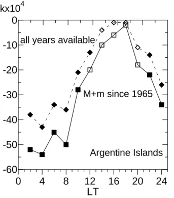
Fig. 1. Value of the foF2 trend k at the Argentine Islands versus local time. Filled diamonds and rectangles show the data significant at the 95% level, according to the Fisher criterion, except for the 0000–1000 LT interval for all years (diamonds) where the points have a 99% significance. Open symbols correspond to statistically insignificant data at the confidence level chosen.The main advantage of the method is that, contrary to the method in which the absolute values are used, it is possible to use the long-term changes of the parameters in various LT moments and months, in spite of the strong diurnal and seasonal variations of both foF2 and hmF2. The third degree-polynomial, in respect to the sunspot number R12, was used
as a model. By using data from 22 stations of the global ionospheric network and considering only the years of solar cycle minima and maxima, the trend in foF2 was found to be negative for all stations (e.g. Danilov and Mikhailov, 1999). More information on the method and results for various sta-tions can be found in the above references.
To analyze the trends at the Argentine Islands and Port Stanley stations we used the same method. The data on foF2 were taken from the WDCC1/UK site on the Internet, and the data on hmF2 were kindly presented to us by Martin Jarvis. According to Jarvis et al. (1998), in order to derive hmF2 values from the M3000 parameter, they have used the well-known Bradley and Dudeney (1973) method.
2.1 Critical frequencies
The behavior of the foF2 trends at Argentine Islands is sim-ilar to that found for the stations analyzed by Danilov and Mikhailov (1999a). Figure 1 shows the values of the trend k (in 10−4per year, obtained as the slope of the linear regres-sion line for the δfoF2 change with time, see the line in Fig.
1960 1970 1980 1990
years
-0.14
-0.10
-0.06
-0.02
0.02
0.06
0.10
0.14
Argentine Islands
M+m since 1965 0400 LTfoF2
δ
Figure 2
Fig. 2. Long-term δfoF2 variations for 0400 LT at the Argentine Islands. Solid line is a linear regression over the points. Error bars present the standard deviation of seasonal (over 12 months) scatter of δfoF2.
2). In the same manner as in Danilov and Mikhailov (1998, 1999a), two cases are considered: all the years available and then only the years since 1965 which are around solar max-ima and minmax-ima (designated below in tables and figures as
M + m). Figure 2 shows an example of the δfoF2 change with time for 0400 LT.
One can see from Fig. 1 that there is a stable negative trend even if all the years are considered. The absolute values of k increase if only M + m years since 1965 are considered. For the entire day, except for the 1400–2000 LT interval, the val-ues of k are significant at the 95% confidence level according to the Fisher criterion (for 0000–1000 LT, they are significant at the 99% confidence level).
The annual mean value k(mean) for the Argentine Islands (φ = 53.8◦) is −2.4 · 10−3 per year, which is close to the values for the Juliusruh (φ = 54.4◦, k = −1.6·10−3per year)
and Yakutsk (φ = 51.0◦, k = −3.1·10−3per year) stations,
with close geomagnetic latitudes in the northern hemisphere (see Danilov and Mikhailov, 1999a). Figure 1 also shows that there is a pronounced diurnal variation of k with much larger values during the night and morning hours than during the noon and evening hours. Possible reasons for this variation is discussed later.
Figure 3 shows the diurnal variations of k values for δfoF2 at Port Stanley. If all the years are considered, the trend k is negative for all hours and significant for the 2000–0600 LT interval. The picture is clearly different from that in Fig. 1. First, the maximum magnitude of the negative trend (at
A. D. Danilov and A. V. Mikhailov: F2-layer parameters long-term trends 343
0
4
8
12
16
20
24
LT
-25
-15
-5
Port Stanley
all years available
M+m since 1965
kx10
4
.
Fig.3
Fig. 3. The values of the foF2 trend k at Port Stanley versus LT. Filled diamonds and rectangles show the data significant at the 95% level, according to the Fisher criterion, except for the 2200–0400 LT interval for all years (diamonds) where the points have a 99% significance. Open symbols correspond to statistically insignificant data at the confidence level chosen.0400 LT) is much less than at the Argentine Islands. Second, reduction of the data to the (M + m) years does not lead to any systematic effect: the values of k(M + m) may be both smaller and larger than k(all) and are insignificant (except at 0400 LT), according to the Fisher criterion, mainly due to the reduction of the number of points.
However, the main feature of the k diurnal variation seen in Fig. 1 (higher values of the negative trends at night and early in the morning) is clearly reproduced in Fig. 3 as well. The importance of this fact will be discussed later.
The annual mean values of k(all) and k(M + m) are
−10·10−4and −8·10−4, respectively. It is only a bit lower than corresponding values of k for Karaganda (φ = 40.3◦,
k = −1.2·10−3), Sofia (φ = 41◦, k = −1.7·10−3per year), and Irkutsk (φ = 41.1◦, k = −1.5·10−3per year), which have close geomagnetic latitudes to that of Port Stanley (40.6◦).
Thus, the foF2 data for both stations considered demon-strate a pronounced negative trend with the magnitude nearly the same as obtained for the corresponding φ in the analysis by Danilov and Mikhailov (1999a) for the northern hemi-sphere stations.
The diurnal variations of the foF2 trends for the Port Stan-ley station are principally the same as for the Argentine Is-lands and for the stations studied by Danilov and Mikhailov (1999a). However, the choice of (M + m) years leads neither to an increase in the trend magnitude nor to a stable picture
1 3 5 7 9 11 13
-55
-45
-35
-25
-15
0400 LT
all years
kx10
4
Argentine Islands
Port Stanley
all years
M+m
foF2
3
6
9
12
Fig. 4. Seasonal variations of the foF2 trend k at two stations for 0400 LT.
of the diurnal variations.
Until now, we have considered only the annual mean val-ues of k for various LT. By considering various months, we obtain the picture of the annual variations of k, shown in Fig. 4, for the particular hour 0400 LT, when, according to Figs. 1 and 3, the absolute values of k have a maximum in the di-urnal behavior. One can see from Fig. 4 that the seasonal variation of k at both stations is relatively small if all the data are considered. The choice of (M + m) years for the Ar-gentine Islands increases the k absolute values, but does not change, in principle, the seasonal behavior. At Port Stanley, the k values for (M + m) year selection are mainly insignifi-cant (see Fig. 3); therefore, we do not show for them seasonal variations.
Comparing seasonal variations of k for (M +m) years with those at the stations considered by Danilov and Mikhailov (1999a), we see that the k variations during a year (or, to be exact, the absence of pronounced seasonal variation) at the Argentine Islands agrees well with the k variations at the northern hemisphere stations, with φ = 54 − 64◦ (the top panel of Fig. 3 in Danilov and Mikhailov, 1999a).
The seasonal behavior of k at Port Stanley also demon-strates no pronounced seasonal variations and, in that aspect, differs from the trend behavior at the stations in the geomag-netic latitude interval 41–54◦ (the middle panel of Fig. 3 in Danilov and Mikhailov, 1999a), which shows more pro-nounced seasonal effect in k. It is possible that the processes of the F2 layer formation at Port Stanley may be different
344 A. D. Danilov and A. V. Mikhailov: F2-layer parameters long-term trends
1955
1965
1975
1985
1995
years
-0.06
-0.02
0.02
0.06
Port Stanley
all years
1000 LT
hmF2
G
Fig. 5. Variations of annual mean δhmF2 with time at Port Stanley. The designations are the same as in Fig. 2.
from the usual ones. This may be due, in particular, to the fact that the station is close to the South-Atlantic Geomag-netic Anomaly and, therefore, processes of direct corpuscu-lar ionization may play some role in the F2 layer formation and thus, disturb the “normal” picture of foF2 and hmF2 be-havior.
Since the amplitude of the seasonal variation at both sta-tions is relatively small (much smaller than the amplitude of diurnal variations), we will not come back to this point and consider only annual mean values of k in the further analysis. 2.2 F2-layer maximum heights
Similar analysis was performed for the hmF2 data at the same two stations. An example of δhmF2 variation with time at Port Stanley is shown in Fig. 5. The values of the trends at both stations obtained for two cases (all the years and only the (M + m) years since 1965) are shown in Table 1. Bold numerals show the k values at the 95% significance level, according to the Fisher criterion; the significance of all other values of k are below the latter value.
Table 1 shows that for the Argentine Islands, we obtain no pronounced regular diurnal variation. All the k values have a significance below the 95% level. On the basis of these values, we can only state that the hmF2 trend tends to be positive.
The behavior of k for hmF2 for Port Stanley is quite dif-ferent (see Table 1). First, all the k values obtained for all the years are negative; on the average, there is a stable negative trend of about 10−3per year. There is some tendency for di-urnal variations with lower absolute values of k around noon, and higher values around midnight. Table 1 demonstrates that all the values of k for the (M + m) years are
insignif-100
200
300
400
500
600
hmF2, km
-0.80 -0.60 -0.40 -0.20 0.00tr
en
d
h
mF2
,
km
Port Stanley
Jarvis et al. [1998]Fig. 6. Absolute values of hmF2 trends versus hmF2. Dashed line is a linear regression over the individual 1hmF2 values (points). Solid line represents similar regression over the individual points taken from Fig. 6 in Jarvis et al. (1998). Open rectangles correspond to the case of constant k = −4·10−3per year.
icant at the level considered. Evidently, for some unknown reason, the choice of the (M + m) years does not work in the case of the hmF2 data, as it works for foF2, over the set of the northern hemisphere stations (Danilov and Mikhailov, 1999a) and for the Argentine Islands (see the previous sec-tion). Therefore, in the following analysis of the hmF2 data, we are considering only the “all years” case.
In continuation, we may note that the method used gives negative trends of foF2 for both stations considered. Annual mean k values agree reasonably well with the foF2 trends for the northern hemisphere stations with close geomagnetic lat-itudes. The (M + m) year selection after 1965 increases the values of k at the Argentine Islands, but does not, in prin-ciple, change the picture of the k diurnal behavior. At Port Stanley, most of the k for the (M + m) years are of low sig-nificance.
The picture for the hmF2 trends is different. The Argentine Island data demonstrate an absence of pronounced trends, whereas at Port Stanley, there is a stable negative trend of about 10−3per year.
3 Comparison with the Jarvis at al. (1998) results
The method used here gives the trends in relative units per year. To compare our results with the results of absolute trend determinations, one needs absolute values of the parameters analyzed. One of the important results of the Jarvis et al. (1998) analysis was the determination of the direct relation between the absolute trend 1hm and the value of hmF2 itself. Jarvis et al. (1998) used values for each hour of every month,
Table 1. The hmF2 trend k in 10−4per year LT 00 02 04 06 08 10 12 14 16 18 20 22 Argentine Islands all −01 +01 +01 −02 −06 +01 +08 +09 +05 +09 +01 −03 (M + m) +09 +13 +09 +04 −03 +01 +13 +12 +11 +10 +02 +02 Port Stanley all −13 −07 −03 −10 −10 −10 −05 −07 −06 −02 −11 −11 (M + m) −02 +01 −02 −03 −07 −09 −02 −08 −05 −03 −05 −04
so they had a huge set of points in their Fig. 6.
To simulate their result, we used the values of the rela-tive trends k shown in Table 1 for Port Stanley. To transfer from a relative trend to an absolute one, one has to multiply the former by a corresponding value of hmF2. We arbitrarily took the monthly mean hmF2 values for Port Stanley for 24 LT moments for January 1958 (solar maximum), June 1975 (solar minimum), and January 1989 (solar maximum). The use of the years of solar maxima and minima made it pos-sible to cover a wider range of the hmF2 variations. Multi-plying hmF2 by the corresponding k provided the absolute trend 1hm in km. It is evident that we are able to add to this figure as many points as we wish, using various months and years, but we limited ourselves by the three months indi-cated above, and obtained the points shown in Fig. 6, which are aimed at merely an illustration of the idea.
Thus, points in Fig. 6 show individual values of 1hmF2 obtained in the previously mentioned method and the dashed line is a least square linear regression. This part of Fig. 6 is qualitatively completely similar to Fig. 6 in Jarvis et al. (1998). To make a quantitative comparison, we present in our Fig. 6 a solid line which is taken from Fig. 6 in Jarvis et al. (1998) and shows a similar regression of 1hmF2 versus
hmF2. To avoid complicating the figure, we cannot present
all the original points shown in the Jarvis et al. (1998) Fig. 6 and thus show, only the regression line.
One can see from Fig. 6 that our results reproduce a prin-cipal dependence of the absolute hmF2 trend on hmF2 itself, as obtained by Jarvis et al. (1998), but the slope of our re-gression line (the dashed line) is lower than that of Jarvis et al. (1998). Our slope corresponds to a mean relative trend
kof about −8·10−4per year (in fact, it was the value taken to calculate the absolute values of 1hmF2, as was described above). One can see from Fig. 6 that the slope of the re-gression line (solid line) obtained by Jarvis et al. (1998) is steeper. The rectangles in our Fig. 6 correspond to the rela-tive trend of −4·10−3per year. One can see that the rectangles fit well the regression line taken from Jarvis et al. (1998).
Thus, there is a difference in the slopes k (relative trends) between the 1hmF2 on hmF2 dependencies obtained by Jarvis et al. (1998) and in the present paper. The difference may be due to the different methods of trend determination in both approaches and to the different amount of points used.
But this is not important for the present consideration. The important thing is that actually the dependence of 1hmF2 on
hmF2 found by Jarvis et al. (1998) is just a consequence of
the fact that the relative trend of hmF2 is constant and this leads to an decrease of 1hm with a decrease of hm itself. If the relative trend were absolutely constant (in fact, it is not so as the hmF2 trend does depend on LT, season, magnetic ac-tivity and possibly other factors), Jarvis et al. (1998) would have a direct line in their Fig. 6 (right panel) with the slope equal to −4·10−3per year and no scatter of the points. How-ever, the seasonal, diurnal and other variations of the relative trend (which do exist in reality) determine the scatter of the points relative to this line, which is actually seen in Fig. 6 (right panel) in Jarvis et al. (1998).
In case of the Argentine Islands data, it is difficult to simu-late the Jarvis et al. (1998) results with the data presented in Table 1. One can see that the relative trend k for the Argen-tine Islands changes sign and is of low significance. The left-hand panel of Fig. 6 in Jarvis et al. (1998) shows that about one-third of all 1hmF2 points lie above the zero line, indi-cating positive trends, with the rest showing negative 1hmF2 values. The approximating line in their figure corresponds to about k = −2· 10−3per year. Strong scatter of the
individ-ual points in both parts of that figure shows that actindivid-ually the relative trend k is rather changeable, depending evidently on both LT and season.
We will return back to the problem of the hmF2 trends below, considering the δfoF2 and δhmF2 relation to the Ap index.
4 Analysis of the δfoF2 and δhmF2 variations
In all the analyses described in the previous section, the val-ues of δfoF2 and δhmF2 determined from the experimental data according to Eqs. (1) and (2), respectively, were used to analyze the general tendency of their variation with time to find the slope k of the approximating line. One can see from Figs. 2 and 5 that even when the tendency is well pronounced and there is no doubt of the δfoF2 (or δhmF2) behavior with time, there are considerable deviations of the
δfoF2 and δhmF2 from the regression line. Let us consider
the question in more detail. One should remember that the
346 A. D. Danilov and A. V. Mikhailov: F2-layer parameters long-term trends
0
8
16
24
LT
-0.7
-0.5
-0.3
-0.1
0.1
0.3
0.5
Port Stanley
Argentine Islands
all years
r( foF2, Ap)
G
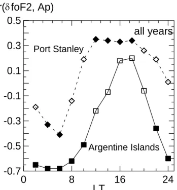
Fig. 7. Diurnal variations of the correlation coefficient r(δfoF2,
Ap12) for the two stations. Filled symbols for the Argentine Island
mean a significance at the 99% level, according to the Fisher crite-rion (except the 2200 LT point which is of the 90% significance). Filled symbols for Port Stanley mean a significance at the 95% level (except the 0400 LT point which is of the 90% significance). Open symbols for both stations mean a significance below 90%.
some model: the foF2 (or hmF2) regression with solar index
R12. Actually, there might be other factors changing from
year to year and leading to deviations of the observed δfoF2 (δhmF2) values from the model, which takes into account only the changes described by R12. The most probable are
two such factors: long-term changes of geomagnetic activ-ity, resulting in long-term trends of the aeronomical parame-ters (neutral composition, temperature, winds), and changes in solar EUV not properly presented by R12variations.
The search for the long-term variations of the F2-layer pa-rameters, in fact, was stimulated by theoretically predicted in the beginning of the 1990s, the changes in foF2 and hmF2 due to the increase in the greenhouse gases in the vicinity of the mesopause and the corresponding cooling of this re-gion (Rishbeth, 1992; Rishbeth and Roble, 1992). Therefore, the results of all attempts to detect the trends in foF2 and/or
hmF2 (see detailed references in Danilov and Mikhailov
(1999a) and the reviews by Danilov (1997,1998)) were in-terpreted in terms of changes of the F-region aeronomical parameters. Danilov and Mikhailov (1999 a.b) were the first to show that the magnitude of the negative trend in foF2 strongly depends on the geomagnetic (not geographic) lati-tude, with the magnitude being higher at high geomagnetic latitudes. This fact put considerable doubts on the “green-house” nature of the trends detected, and led Danilov and Mikhailov (1999a) to assume that these trends may be
re-lated to the trends in the occurrence of ionospheric storms, as reported by a group of authors (Sergeenko and Kuleshova, 1994, 1995; Sergeenko and Givishvily, 1997). Mikhailov and Marin (2000) analyzed the relation of the foF2 behav-ior to geomagnetic activity and demonstrated that the annual mean values of δfoF2 at three stations (Slough, Moscow, and Tomsk) correlate to the annual mean values of the Ap geo-magnetic index. This does not mean that there cannot exist other foF2 and hmF2 trends of the “greenhouse” or other na-ture, but the input of the geomagnetic trend into foF2 and
hmF2 long-term changes seems evident.
Coming back now to the analysis of the Argentine Islands and Port Stanley data, we will analyze individual values of
δfoF2 and δhmF2 to determine whether they present merely
random deviations from the smooth behavior described by the model, or one or both factors mentioned above play a part in determining their behavior.
4.1 Comparison with geomagnetic activity
To analyze the relation of the δfoF2 and δhmF2 values with geomagnetic activity, we used the annual mean values of the Ap12 geomagnetic index. These values were compared
with δfoF2 and δhmF2 for each particular situation consid-ered and the corresponding correlation coefficients were cal-culated. Since the diurnal variations of both parameters are better pronounced than the seasonal ones (see the previous section), we used the annual mean δfoF2 and δhmF2 values and considered only the diurnal variations. We have found that the choice of (M + m) years since 1965 in the δhmF2 case does not lead to any significant difference in the corre-lation coefficient obtained; thus, we considered all the data, because in this case, the statistical provision of the results is much better.
Figure 7 shows the correlation coefficient r(δfoF2, Ap12)
for both stations as a function of the local time. Several fea-tures of Fig. 7 should be noted: 1) there is an evident sim-ilarity in the diurnal behavior of r(δfoF2, Ap12) at both
sta-tions. It may be considered as a first proof that the δfoF2 values are not merely occasional deviations from the model but, at least partly, are a manifestation of the magnetic ac-tivity not taken into account in the model; 2) there is an im-portant feature in both curves: the values of r(δfoF2, Ap12)
are positive in the afternoon and negative at midnight and in the early morning periods; 3) at the Argentine Islands, the maximum positive value of r(δfoF2, Ap12) is relatively small
(around 0.1) and insignificant. In fact, Fig. 7 shows that in the afternoon and early evening periods, there is practically no significant correlation between δfoF2 and Ap12. Contrary
to that, the negative correlation between δfoF2 and Ap12
dur-ing the night is well pronounced (the value of r bedur-ing about 0.6–0.7 during several hours) and statistically significant; 4) at Port Stanley, the values of the r(δfoF2, Ap12) are about
0.3 and −0.4 in the afternoon maximum and early morning minimum, respectively. The difference in the two curves in Fig. 7 encourages us to assume that the mechanisms of the magnetic influence on foF2 at the two stations are different,
which may be due to the fact that Port Stanley is close to the region of the South-Atlantic Geomagnetic Anomaly and additional sources of ionization may govern the F2-region behavior there.
4.2 Possible relation to ionospheric storms
Now we try to consider all the experimental evidence de-scribed above in terms of the hypothesis that long-term chan-ges in geomagnetic activity (and corresponding number and intensity of ionospheric storms) is the most probable cause of the described behavior of δfoF2 and δhmF2.
According to the contemporary understanding of the iono-spheric storm physics and morphology (see the reviews by Pr¨olls, 1995; Field and Rishbeth, 1998; Rees, 1995; Danilov, 2000), the principal scheme of an ionospheric storm looks like the following: the Joule heating in the auroral zone changes the thermospheric composition (in-creases the molecule-to-atom ratio), in(in-creases the neutral gas temperature and generates storm-induced global circulation. Changes in the aeronomical parameters ([N2]/[O] and T )
lead to a decrease of the electron concentration (or foF2) in the heated gas. This is the negative phase of an iono-spheric storm. The storm-induced circulation tends to bring the heated gas from the auroral zone equatorward to lower latitudes. How far this gas really penetrates down the lati-tudes depends on the competition between the storm-induced and normal (solar driven) circulation. The latter depends on season and local time. During the daytime, in winter, the so-lar driven circulation is directed poleward and thus, opposite to the storm-induced circulation. In this case, the heated gas may stay “locked” in the zone of the Joule heating or drift only slightly to lower latitudes. In the night the situation is different. The solar driven background circulation is weak-ened and can no longer completely stop the storm-induced circulation; the gas with changed temperature and composi-tion moves down the latitudes and the negative phase may be observed at relatively low latitudes (down to φ = 35 − 40◦). In summer the storm-induced and solar-driven background circulation coincide practically all day long and thus, the heated gas reaches low enough latitudes. Two points of the described simplified scheme are important for our analysis. First, at moderate latitudes, the negative phase, on the whole, is observed more often than the positive one. Second, the most favorable conditions for the negative phase occurrence are at night and early in the morning, when in all seasons, the storm-induced circulation is able to penetrate to moderate latitudes and bring the heated gas with changed temperature and composition.
Let us consider how, in this paper as well as in Danilov and Mikhailov (1999a, b), Mikhailov and Marin (2000), the revealed features of the δfoF2 and δhmF2 behavior can be interpreted in terms of long-term variations in geomagnetic activity and related changes in number and intensity of iono-spheric storms.
As it was mentioned earlier, the negative phase of an iono-spheric storm is observed mostly at night. Therefore, one
0
4
8
12
16
20
24
LT
0.0
0.2
0.4
0.6
correl
ation
c
oe
ff
icien
t
Port Stanley
Argentine Islands
0Figure 8.
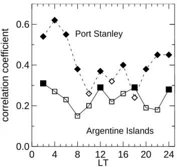
Fig. 8. Diurnal variations of the correlation coefficient r(δhmF2,
Ap12) for the two stations. Filled symbols for the Argentine Island mean a significance at the 90% level, according to the Fisher cri-terion. Filled symbols for Port Stanley mean a significance at the 95% level (except the 2200–0600 LT interval where the points are of the 99% significance). Open symbols for both stations mean a significance below 90%.
would expect negative foF2 trends to be better pronounced at night and early in the morning. This is exactly what we see in Fig. 1 for the Argentine Islands. This station lies at the latitude where, according to the analysis of the latitude dependence of the foF2 trends by Danilov and Mikhailov (1999a) and Mikhailov and Marin (2000), the negative phase effects should be well manifested. The diurnal behavior of k for δfoF2 at the Argentine Islands agrees well with that for Moscow, as obtained by Mikhailov and Marin (2000) for the period after 1965. The maximum negative trends of about
−0.003 per year were found there at 0000–0600 LT and the minimum trends of about −0.001 per year are seen in the afternoon hours.
Thus, diurnal variations of the foF2 trends at the Argentine Islands agree with the assumption that the negative trends may be due to an occurrence frequency increase of the iono-spheric storm negative phase. The analysis of the δfoF2 cor-relation with Ap12(Fig. 7) also works in the same direction.
The strongest (negative!) correlation is seen in the midnight-early morning period, whereas in the daytime, the correlation coefficient changes sign and is small in magnitude.
The diurnal variation of k at Port Stanley (Fig. 3) is not as regular as that at the Argentine Islands. Nevertheless, the principal for our consideration feature, a strong nighttime maximum, does exist, thus, confirming the previous conclu-sion. The correlation coefficient of δfoF2 with Ap12(see Fig.
7) shows the same type of diurnal variation as at the Argen-tine Islands, but with different values. Negative values of
348 A. D. Danilov and A. V. Mikhailov: F2-layer parameters long-term trends period of relatively low but stable positive correlation in the
daytime.
We think that the features described above in the diurnal variations of k and r(δfoF2, Ap12) at Port Stanley are a
mani-festation of a peculiar ionization cycle governing the electron concentration behavior at this station. Probably an increase of the magnetic activity enhances corpuscular ionization of the F2-region. If this is true, two factors affect the behavior of foF2 when Ap12 is increasing: the effect of ionospheric
storm negative phase should be reduced (that is exactly what we see at night) and there should be even positive correla-tion with Ap12 in the daytime, when the probability of the
negative phase occurrence is relatively low.
Also understandable in the scope of the simplified scheme of the ionospheric storm development described seems to be the behavior of two correlation coefficients during the night. We have already mentioned that this period is the most favor-able for penetration of the storm-induced circulation down the latitudes. The equatorward wind, along with an increase of β (due to γ1,2, [N2], and [O2]), results in the hmF2
in-crease. Here, β is the linear recombination coefficient, and
γ1and γ2are the rate constants of the reactions of O+with
N2and O2molecules, respectively. At the same time, the
in-crease of β should lead to a dein-crease in foF2, which is man-ifested by a strong negative correlation between δfoF2 and
Ap12in Fig. 7 for this period.
Figure 7 shows that diurnal variations of the correlation coefficient r(δfoF2, Ap12) are similar for both stations. The
only difference is that at the Argentine Islands, the daytime maximum of r(δfoF2, Ap12) is narrow and has smaller
ampli-tude than at Port Stanley. This may be due to the fact that the geomagnetic latitude of the Argentine Islands is significantly higher than that of Port Stanley; thus, the effect of the heated gas from high latitudes should be stronger at the former sta-tion, leading to a larger input of the negative phase and thus, leading to a general shift of the r(δfoF2, Ap12) curve in Fig.
7 in the direction of negative correlation.
Variations of hmF2 during ionospheric storms are control-led by increased neutral temperature Tn, linear loss
coeffi-cient β = γ1[N2] +γ2[O2], and vertical plasma drift related
to thermospheric winds and electric fields. Magnetospheric electric fields produce short-term hmF2 variations and may not be considered in the long-term trend analysis. The first three parameters are known to increase during disturbed pe-riods, resulting in the hmF2 increase at middle and lower lat-itudes (Mikhailov et al., 1995).
For this consideration, it is important that during ionosphe-ric storms, hmF2, in almost all cases, should increase. There-fore, one would expect only a positive correlation between
δhmF2 and magnetic activity. This was also shown by Marin
et al. (2001) for many northern hemisphere stations. Actu-ally, positive values of r(δhmF2, Ap12) are seen at both
sta-tions in Fig. 8. The correlation coefficient of δhmF2 with
Ap12 at Port Stanley is significant for most of the LT
mo-ments and higher at night (0.5–0.6) than in the daytime. The values of r(δhmF2, Ap12) at the Argentine Islands are much
lower and insignificant.
In spite of the positive correlation between δhmF2 and
Ap12, negative long-term trends of hmF2 at Port Stanley are
obtained both in Jarvis et al. (1998) and this paper. Since there is a well-known long-term increase of magnetic activ-ity (see e.g. Clilverd et al., 1998), one would expect a posi-tive trend of hmF2. However, the Port Stanley is a peculiar station. Since it is in the vicinity of the South-Atlantic Mag-netic Anomaly, the magMag-netic storms at this station may be manifested not only by the aeronomical parameter changes discussed above, but also by corpuscular precipitation. Such precipitation would increase the ionization rate q and change the electron concentration vertical profile in the entire F re-gion, shifting it down in such a way that the maximum of the electron concentration would tend to be lower than in quiet conditions. It is evident that this effect, if it exists, should be pronounced at high-latitude stations, where magnetic distur-bances are accompanied by particle precipitation. In fact, the same effect of negative trends have been found by Marin et al. (2001) for several high-latitude stations and above all, for Sodankyla.
5 Conclusions
In this paper we applied the method developed and described earlier to look for long-term trends of the F2-layer parame-ters (foF2 and hmF2) at two southern hemisphere ionospheric stations, the Argentine Island and Port Stanley, recently con-sidered by Jarvis et al. (1998). The main results of our anal-ysis may be listed as follows:
1. Negative foF2 trends are observed at both stations. The average value of the trend k for the Argentine Island is −2.4· 10−3per year, which is close to the values of k obtained for the stations with similar geomagnetic latitude in the north-ern hemisphere. For Port Stanley, the averaged value k =
−8·10−4per year is also only slightly lower than the k val-ues for the corresponding stations considered by Danilov and Mikhailov (1999b). It is worth noting that the principal con-clusions based on the analysis of the northern hemisphere stations are confirmated: the foF2 trends are negative and demonstrate a pronounced diurnal behavior.
2. The diurnal variation of k for foF2 at the Argentine Island is well pronounced and similar to the diurnal varia-tions at the corresponding northern hemisphere stavaria-tions, with maximum amplitudes of the negative trend at night and in the early morning hours, and a minimum in the afternoon. The diurnal variation of k at Port Stanley is less systematic (es-pecially during daytime), but shows a pronounced maximum at night. The irregularity of the diurnal behavior of k at Port Stanley may be due to its peculiar position close to the South Atlantic Geomagnetic Anomaly.
3. The increase of the magnitude of the absolute trend
1hmF2 with an increase in hmF2 itself, found by Jarvis et
al. (1998) for Port Stanley, is merely a manifestation of a relative constancy of the relative trend which, in this case, is equal to −4·10−3per year.
cor-relation coefficients between δfoF2, δhmF2 and Ap12shows
that they principally agree with the current understanding of ionospheric storm physics and morphology. This means that the long-term trend in ionospheric storms found by various authors can contribute significantly to the long-term trends in
foF2 and hmF2 and mask significantly the effects (if any) of
a greenhouse gas increase.
Acknowledgements. The authors thank Dr. M. Jarvis for providing
the hmF2 data and discussion of the paper.
Topical Editor M. Lester thanks C. Davis and J. Lastovicka for their help in evaluating this paper.
References
Bencze, P., Sole, G., Alberca, L. F., Poor, A., Long-term changes of hmF2 possible latitudinal and regional variations, Proc. 2nd COST 251 Workshop “Algorithms and Models for COST 251 Final Product”, Rutherford Appleton Lab., UK, 107–113, 1998. Bradley, P. A. and Dudeney, J. R., A simple model of the vertical
distribution of electron concentration in the ionosphere, J. At-mos. Terr. Phys. 35, 2131–2146, 1973.
Bremer, J., Some additional results of long-term trends in vertical-incidence ionosonde data, Paper presented at the COST 251 Meeting, Prague, September 1996.
Bremer J., Trends in the ionospheric E and F regions over Europe, Ann. Geophysicae, 16, 986–996, 1998.
Danilov, A. D., Long-term changes of the mesosphere and lower thermosphere temperature and composition, Adv. Space Res., 20, 2137–2147, 1997.
Danilov, A. D., Review of long-term trends in the upper meso-sphere, thermomeso-sphere, and ionomeso-sphere, Adv. Space Res., 22, 907– 915, 1998.
Danilov, A. D., F-region reaction to magnetospheric storm, J. At-mos. Terr. Phys., in press, 2000.
Danilov, A. D. and Mikhailov, A. V., Long-term trends of the F2-layer critical frequencies: a new approach, Proc. 2nd COST 251 Workshop “Algorithms and Models for COST 251 Final Prod-uct”, Rutherford Appleton Lab., UK, 114–121, 1998.
Danilov, A. D. and Mikhailov, A. V., Spatial and seasonal variations of the foF2 long-term trends, Ann. Geophysicae, 17, 1239–1243, 1999a.
Danilov, A. D. and Mikhailov, A. V., Long-term trends of the F2-layer parameters: a new approach, Int. Journ. Geomag. Aeron. (http://eos.wdcb.rssi.ru/ijga), 1, (3), 1999b.
Field, P. R., Rishbeth, H., Moffett, R. J. et al., Modeling composi-tion changes in F-layer storms, J. Atmos. Solar Terr. Phys., 60, 523–543, 1998.
Givishvili, G. V. and Leshchenko, L. N., Long-term trends of the properties of the midlatitude ionosphere and thermosphere, Dokl. RAN (in Russian), 333 (1), 86–92, 1993.
Givishvili, G. V. and Leshchenko, L. N., Possible proof of the pres-ence of technogenic impact on the midlatitude ionosphere, Dokl.
RAN (in Russian), 334 (2), 213–214, 1993.
Jarvis, M. J., Jenkins, B., and Rogers, G. A., Southern hemisphere observations of a long-term decrease in F region altitude and thermospheric wind providing possible evidence for global ther-mospheric cooling, J. Geophys. Res., 103, 20744–20787, 1998. Klilverd, M. A., Clark, T. D. G., Clarke, E., and Rishbeth, H.,
In-creased magnetic storm activity from 1968 to 1995, J. Atmos. Terr. Phys., 60, 1047–1056, 1998.
Marin, D., Mikhailov, A. V., de la Morena, B. A., and Herraiz, M., Long-term hmF2 trends in the Eurasian longitudinal sector on the ground-based ionosonde observations, Ann. Geophysicae, sub-mitted, 2001.
Mikailov, A. V., Skoblin, M. G., and F¨orster, M., Daytime F2-layer positive storm effect at middle and lower latitudes, Ann. Geo-physicae, 13, 532–540, 1995.
Mikhailov, A. V. and Marin, D., Geomagnetic control of the foF2 trends, Ann. Geophysicae, 18, 653–665, 2000.
Mikhailov, A. V. and Marin, D., An interpretation of the foF2 and
hmF2 long-term trends in the framework of the geomagnetic
con-trol concept, Ann. Geophysicae, submitted, 2001.
Pr¨olls, G., Ionospheric F-region storms, in Handbook of Atmo-spheric Electrodynamics, Vol 2, Ed. H. Volland, CRC Press/Boca Raton, 195–248, 1995.
Rees, D., Observations and modeling of ionospheric and thermo-spheric disturbances during major geomagnetic storms: A re-view, J. Atmos. Terr. Phys., 57, 1433, 1995.
Rishbeth, H., A greenhouse effect in the ionosphere? Planet. Space Sci., 38, 945–948, 1990.
Rishbeth, H., How the thermospheric circulation affects the iono-spheric F2-layer, J. Atmos. Solar Terr. Phys., 60, 1385–1402, 1998.
Rishbeth, H. and Roble, R. G., Cooling of the upper atmosphere by enhanced greenhouse gases – Modeling of thermospheric and ionospheric effects, Planet. Space. Sci., 40, 1011–1026, 1992. Sergeenko, N. P. and Kuleshova, V. P., Long-term trends in
iono-spheric disturbances in the F2 region, Geomag. Aeronom. (in Russian), 35(5), 128–130, 1995.
Sergeenko, N. P. and Kuleshova, V. P., Climatic changes of the prop-erties of disturbances in the ionosphere and upper atmosphere, Dokl. RAN (in Russian), 334 (4), 534–536, 1994.
Sergeenko, N. P. and Givishvili, G. V., On the problem of many-year properties of ionospheric disturbances, Geomag. Aeronom. (in Russian), 37(2), 108–113, 1997.
Ulich, T. and Turunen, E., Evidence for long-term cooling of the upper atmosphere in ionospheric data, Geophys. Res. Lett., 24, 1103–1106, 1997.
Ulich, T., Karinen, A., and Turunen, E., Effects of solar variability seen in long-term EISCAT radar observations of the lower iono-sphere, Paper presented at the Second IAGA/CMA Workshop on Solar Activity Forcing ofthe Middle Atmosphere, Prague, Au-gust 1997.
Upadhyay, H. M. and Mahajan, K. K., Atmospheric greenhouse ef-fect and ionospheric trends, Geophys. Res. Lett. 25, 3375–3378, 1988.