HAL Id: hal-00298095
https://hal.archives-ouvertes.fr/hal-00298095
Submitted on 12 Nov 2007
HAL is a multi-disciplinary open access
archive for the deposit and dissemination of
sci-entific research documents, whether they are
pub-lished or not. The documents may come from
teaching and research institutions in France or
abroad, or from public or private research centers.
L’archive ouverte pluridisciplinaire HAL, est
destinée au dépôt et à la diffusion de documents
scientifiques de niveau recherche, publiés ou non,
émanant des établissements d’enseignement et de
recherche français ou étrangers, des laboratoires
publics ou privés.
time slices
J. O. Sewall, R. S. W. van de Wal, K. van der Zwan, C. van Oosterhout, H. A.
Dijkstra, C. R. Scotese
To cite this version:
J. O. Sewall, R. S. W. van de Wal, K. van der Zwan, C. van Oosterhout, H. A. Dijkstra, et al..
Climate model boundary conditions for four Cretaceous time slices. Climate of the Past, European
Geosciences Union (EGU), 2007, 3 (4), pp.647-657. �hal-00298095�
© Author(s) 2007. This work is licensed under a Creative Commons License.
of the Past
Climate model boundary conditions for four Cretaceous time slices
J. O. Sewall1,*, R.S.W. van de Wal1, K. van der Zwan2, C. van Oosterhout3, H. A. Dijkstra1, and C. R. Scotese4
1Institute for Marine and Atmospheric Research Utrecht, Utrecht University, Princetonplein 5, 3584 CC Utrecht, The Netherlands
2Faculty of Geosciences, P.O. Box 80021, 3508 TA Utrecht, The Netherlands
3Shell International Exploration and Production, P.O. Bos 60, 2280 Rijswijk, The Netherlands
4PALEOMAP Project, Department of Earth and Environmental Sciences, Univ. of Texas at Arlington, Texas, 76019, USA *now at: Department of Geosciences, Virgina Tech, 4044 Derring Hall (0420) Blacksburg, VA 24061, USA
Received: 14 May 2007 – Published in Clim. Past Discuss.: 4 June 2007
Revised: 27 September 2007 – Accepted: 30 October 2007 – Published: 12 November 2007
Abstract. General circulation models (GCMs) are useful
tools for investigating the characteristics and dynamics of past climates. Understanding of past climates contributes significantly to our overall understanding of Earth’s climate system. One of the most time consuming, and often daunt-ing, tasks facing the paleoclimate modeler, particularly those without a geological background, is the production of surface boundary conditions for past time periods. These bound-ary conditions consist of, at a minimum, continental con-figurations derived from plate tectonic modeling, topogra-phy, bathymetry, and a vegetation distribution. Typically, each researcher develops a unique set of boundary condi-tions for use in their simulacondi-tions. Thus, unlike simula-tions of modern climate, basic assumpsimula-tions in paleo surface boundary conditions can vary from researcher to researcher. This makes comparisons between results from multiple re-searchers difficult and, thus, hinders the integration of stud-ies across the broader community. Unless special changes to surface conditions are warranted, researcher dependent boundary conditions are not the most efficient way to pro-ceed in paleoclimate investigations. Here we present sur-face boundary conditions (land-sea distribution, paleotopog-raphy, paleobathymetry, and paleovegetation distribution) for four Cretaceous time slices (120 Ma, 110 Ma, 90 Ma, and 70 Ma). These boundary conditions are modified from base datasets to be appropriate for incorporation into numerical studies of Earth’s climate and are available in NetCDF format upon request from the lead author. The land-sea distribution, bathymetry, and topography are based on the 1◦×1◦(latitude
× longitude) paleo Digital Elevation Models (paleoDEMs)
of Christopher Scotese. Those paleoDEMs were adjusted us-ing the paleogeographical reconstructions of Ronald Blakey
Correspondence to: J. O. Sewall
(Northern Arizona University) and published literature and were then modified for use in GCMs. The paleovegetation distribution is based on published data and reconstructions and consultation with members of the paleobotanical com-munity and is represented as generalized biomes that should be easily translatable to many vegetation-modeling schemes.
1 Introduction
Over the last few decades, the use of numerical models to investigate Earth’s climate history has increased; as those models have grown in sophistication, resolution, and com-plexity, the level of informational input that they require has also grown (Barron, 1984; Sloan and Barron, 1992; Huber and Sloan, 2001; Otto-Bliesner et al., 2002; DeConto and Pollard, 2003; Sewall and Sloan, 2006). At the most basic level, all General Circulation Models (GCMs) run on a rep-resentation of the physical Earth. Basic geography, elevation, and bathymetry must be defined. In addition, in many mod-els (e.g. ECHAM5, CCSM3; Jungclaus et al., 2005; Collins et al., 2006) the characteristics of the land surface (soil con-ditions, vegetation distribution, locations of land ice, river runoff paths etc.) must also be defined. While all of these quantities are relatively easy to obtain for the present day, re-searchers simulating paleoclimates can face a daunting and time consuming task when developing surface boundary con-ditions.
The production of such boundary conditions frequently in-volves a comprehensive search of the literature for published estimates of elevations, ocean depths, continental locations, and vegetation types in a specific time period. These, of-ten limited, data points are then integrated with general, re-gional geological and biological information to build a suite
of boundary conditions from scratch (e.g. Bice et al., 1998; Hay and Wold, 1998; Sewall et al., 2000; Markwick and Valdes, 2004). This time consuming and complex task is of-ten completed by researchers with geological and paleonto-logical training. However, as more and more researchers fo-cus on understanding Earth’s climate history through numer-ical modeling, an increasing proportion of those researchers have backgrounds in other, equally important, disciplines (e.g. Mathematics, Physics, Atmospheric Dynamics, Physi-cal Oceanography), and for those researchers, generating ap-propriately detailed boundary conditions for a given time in Earth’s history can be an especially challenging task. In ad-dition, while sensitivity studies investigating the influence of changing surface conditions on climate are an integral part of understanding climatic conditions in the past, many pale-oclimate investigations would benefit from a common set of surface boundary conditions. Such common boundary condi-tions would permit clearer comparisons between work from multiple research groups and would encourage greater ease and progress toward integrating a community-wide under-standing of the climate system in a given time period.
To this end, we present climate model boundary condi-tions for four Cretaceous time slices generated as part of a study focused on understanding the dynamics and his-tory of anoxic events in the Cretaceous oceans. Those time slices are: the early Aptian (∼120 Ma±5 Ma), the early Albian (∼110 Ma±5 Ma), the Cenomanian/Turonian boundary (∼90 Ma±5 Ma) and the early Maastrichtian (∼70 Ma±5 Ma); an excellent description of the concept of a time slice can be found in Markwick and Valdes (2004). These four time slices represent three times in earth his-tory known to contain widespread ocean anoxia (early Ap-tian, early Albian, Cenomanian/Turonian boundary) and one “control” time that is not (Maastrichtian). We present the essence of our geographical, topographic, and vegetative boundary conditions in this paper, and the boundary condi-tion files are available upon request. In disseminating these boundary conditions, it is our intent to aid other researchers interested in investigating Cretaceous climates and, thus, fa-cilitate a greater and more rapid understanding of some of the outstanding and integral questions in the dynamics of green-house climates.
2 Methods
We begin creating our Cretaceous boundary conditions with the global geography, topography, and bathymetry for each time slice. We alter these base datasets to incorporate new information and to render them appropriate for use in GCMs. On top of this physical surface, we then layer the appro-priate land surface by including land ice, vegetation, sur-face runoff paths, and soil conditions. The base datasets for global geography, topography, and bathymetry for all four of our Cretaceous time slices were obtained from the
PALEOMAP project’s set of 50 Phanerozoic, 1◦latitude × 1◦longitude, paleo Digital Elevation Models (paleoDEMS); in some instances the paleoDEMs were modified based on published literature and the paleogeographical recon-structions of Ronald Blakey (http://jan.ucc.nau.edu/∼rcb7/ globaltext2.html). From this basis, datasets were first con-verted into NetCDF format and interpolated to a resolution of ∼2.8◦latitude × 2.8◦longitude (∼280 km×280 km) using the NCAR Command Language (NCL; http://www.ncl.ucar. edu/). The NetCDF datasets were then manipulated using MATLAB with MEXNC and the NetCDF Toolbox installed (http://mexcdf.sourceforge.net/). Modifications to the origi-nal datasets included merging differing paleogeographical or topographical elements and altering the geography, topogra-phy and bathymetry such that they can easily be incorporated as the lower boundary condition of a GCM.
These alterations are specifically: (1) The removal of marginal seas (ocean areas with limited or no connection to the global ocean) – as they are not connected to the global ocean, marginal seas present problems for the conservation of water in earth system models without an explicit lake com-ponent (which covers most GCMs). In the advent of a sig-nificant marginal sea, either a gateway must be opened to connect it to the global ocean or an artificial restoring flux between the marginal sea and the global ocean must be spec-ified. In instances where the connection between a marginal sea and the global ocean is below the functional model res-olution, we consider that the error incorporated by removing that sea wholesale is less than that introduced by arbitrarily specifying a flux between that marginal sea and the global ocean and, thus, we remove the marginal sea. (2) The ex-pansion of narrow ocean gateways to allow unrestricted flow – depending on the location of velocity points in an ocean grid (grid center or grid corner) it is necessary to have at least one and in many cases two or three ocean grid points in width and one to three grid points in depth to ensure ac-tual flow through a narrow gateway. In our case we expand all ocean gateways to three grid cells in width and two grid cells in depth (840 km wide × 25 m deep at our operational resolution) in order to ensure flow. This same process ap-plies to alteration (3), the merging of island clusters without sufficient flow between islands. Just as in gateways between large continental land masses, we open flow between islands to three grid points in width and two grid points in depth. If the islands in question were too small to have a strait of this size between them, we merged clusters of islands together into one, or more, larger island(s). Alteration (4) made to the base datasets was the removal of areas of internal drainage on continents. Like marginal seas, in models without a spe-cific lake component, internal drainage poses difficulties for the conservation of water within a model. In all instances where internal drainage on a continent occurred, we rerouted the runoff from this depression to the nearest, downslope ocean basin. While we note that features such as those de-scribed above may well be realistic aspects of the
paleogeog-Table 1. Summary of generalized biomes in the Cretaceous vegetation scheme.
High altitude/latitude, evergreen, conifer, closed canopy forest
High altitude/latitude mixed forest with equal percentage of broad and needle leaved and evergreen and deciduous trees Low altitude/latitude, evergreen, conifer,
closed canopy forest
Closed canopy, broad leaved, moist,evergreen forest Closed canopy, broad leaved, dry,
deciduous forest
savanna (dry, low understory with sparse,broad leaved overstory) High altitude/latitude, moist, open
canopy, evergreen forest with a shrub understory
Low altitude/latitude, moist, open canopy, mixed evergreen/deciduous, forest with a shrub understory
Wet or cool evergreen shrubland Dry or warm deciduous shrubland
raphy/topography, they pose numerical problems for GCMs (e.g. Wajsowicz, 1995, 1996) and must be removed in the production of functional boundary conditions. In addition, the relatively coarse spatial resolution of GCMs prohibits the resolution of geographical details and, consequently, model boundary conditions must always be a smoothed approxi-mation of the actual paleo land surface. Finally, in many past times, the available data density is at a resolution even coarser than that of the GCM and, as such, increased model resolution to capture “details” in many cases provides more grid boxes but no additional information.
In all time slices, the most extensive modifications made to the paleogeographic reconstructions were in the geograph-ically complex regions of western Eurasia, Tethys, the South Atlantic, and the South Polar region. In all instances, the complexity of the geography was reduced to create fewer landmasses and larger, better-defined ocean regions to al-low for more accurate numerical modeling of the global earth system.
Global vegetation distributions for each of the four time slices were created in MATLAB by hand and are based on published paleobotanical data (Aptian: Vakhrameev, 1991; Saward, 1992; Archangelsky, 2001; Mohr and Rydin, 2002; van Waveren et al., 2002; Archangelsky, 2003) (Albian; Vakhrameev, 1991; Saward, 1992; Spicer and Herman, 2001; Mohr and Rydin, 2002; Spicer et al., 2002) (Ceno-manian/Turonian: Saward, 1992; Spicer et al., 2002; Wing, 2006 personal communication) (Maastrichtian: Vakhrameev, 1991; Saward, 1992; Mohr and Lazarus, 1994; Otto-Bliesner and Upchurch, 1997; van der Ham et al., 2003) and recon-structions (Spicer and Chapman, 1990; Vakhrameev, 1991; Saward, 1992; Spicer and Corfield, 1992; Otto-Bliesner and Upchurch, 1997). The vegetation types used have been gen-eralized from those of the NCAR Land Surface Model (Bo-nan, 1998) in an effort to make them broadly applicable to both our degree of understanding of Cretaceous
vegeta-tion distribuvegeta-tions and the varying vegetavegeta-tion schemes em-ployed in different land surface models. Given the limited data on Early Cretaceous global vegetation distributions and the significant evolutionary changes in plants during that epoch (Crane et al., 2002), we specify vegetation in func-tional biomes – groupings of plants that, regardless of biol-ogy, probably had the same community structure and climate influence. In addition, those biomes were created to be as general and inclusive as possible while still maintaining sig-nificant differences (from a climatological point of view) be-tween different biomes. The ten biomes represented in our vegetation scheme are summarized in Table 1 and the ba-sis from which our biomes are derived is further described in Bonan (1996). We furthermore expect climate patterns in the Cretaceous to follow some of the same, large-scale, physical constraints that we see today. Temperature is ex-pected to decrease with increasing latitude and/or elevation. Areas of large scale convergence and descending air are ex-pected to be dryer (∼30◦N and S latitude and in polar re-gions), while areas of large scale divergence and ascending air are expected to be wetter (∼50◦N and S latitude and near the equator). Maritime climates are generally expected to be milder with less seasonality than continental interior cli-mates at comparable latitudes. Large topographic features are expected to create rain shadows and dryer conditions on their leeward side. After entering published vegetation data points or reconstructions into MATLAB, the vegeta-tion type was altered to match one of the available types in our scheme. The areas between published tie points were filled based on the expected, large-scale climate patterns out-lined above, published reconstructions (Vakhrameev, 1991; Saward 1992; Otto-Bliesner and Upchurch, 1997), and inter-polation between related data points.
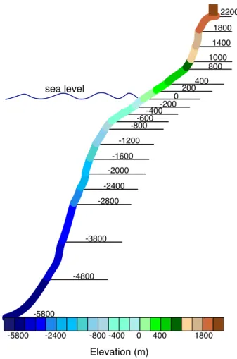
-5800 -2800 -800 400 2200 1800 1400 1000 800 200 0 -200 -400 -600 -1200 -1600 -2000 -2400 -3800 -4800 -5800 -2400 -800 -400 0 400 1800 Elevation (m) Figure 1 sea level
Fig. 1. Detailed key of topography and bathymetry. Blue colors
in-dicate ocean while greens and browns represent land. Darker blues are deep water, lighter blues are shallow. Lower elevation land is represented in greens and higher elevations are brown. In general, the contour interval is greater at the extremes of the color bar and smaller near the land/sea boundary.
3 Boundary conditions
The boundary conditions for each of the four time slices are presented here graphically and time or geographically spe-cific alterations to and notable features of individual recon-structions are detailed in the text. For each time slice, views of the geography, topography, and bathymetry are presented in cylindrical equidistant projection and in two polar projec-tions (North and South Poles) with an equatorward limit of 30◦N/S. The color bar on all plots is the same and increases nonlinearly in an effort to highlight important aspects of the topography. A detailed representation of the color scale used in the topographic plots is found in Fig. 1. Elevations in all time slices range from −5800 m to ∼2200 m.
Early Aptian geography, topography, and bathymetry are presented in Fig. 2. Important features of the Aptian geogra-phy, topogrageogra-phy, and bathymetry include, the lack of a major land mass at the South Pole, an Arctic Ocean with relatively
extensive, though shallow, connections to the global oceans, a small North Atlantic, a minimal, extremely shallow South Atlantic, and a narrow sea strait between southeastern Africa and India. The highest elevations are in Central Asia with other minor highs of note in the proto Andean Arc and the proto Cordillera of North America.
For the early Aptian, we created a south polar land mass (absent in the paleogeographical reconstruction) to avoid the pole problem in ocean models. [All lines of longi-tude converge at the poles in a standard, rectilinear, lat-itude × longlat-itude grid. When solving differential equa-tions via a finite difference approach, this convergence of grid boxes to a single point results in numerical instabili-ties. For ocean modeling, if the poles are located in land masses, this difficulty can be avoided. All of our geogra-phies are constructed assuming a single pole in the Southern Hemisphere and the ability to move the north pole to Green-land or generate a tripolar grid with one Northern Hemi-sphere pole in Eurasia and one in North America.] In addi-tion, while the reconstructions of Blakey (http://jan.ucc.nau. edu/∼rcb7/globaltext2.html), Meschede and Frisch (1998), and Ross and Scotese (1988) indicate islands in the Panama Strait at this time, more recent reconstructions by Scotese (www.scotese.com; Scotese, 2001) do not. Primarily be-cause islands limit, if not prohibit, flow through this nar-row gateway, we choose to exclude them from our bound-ary conditions. The reconstructions of Blakey and Scotese also disagree on the presence of a Cretaceous Interior Seaway in Western North America in the early Aptian. As a partial seaway is undoubtedly present in the Albian and a full sea-way present at the Cenomanian/Turonian boundary, we opt to exclude the Western North American Cretaceous Interior Seaway from our Aptian boundary conditions such that our boundary conditions through the Early Cretaceous represent a suite of possible seaway configurations (no seaway in the early Aptian, a partial seaway in the early Albian, and an ex-tensive seaway at the Cenomanian/Turonian boundary); this is done in order to gain a general impression of the sensitivity of modeled flow to changing geographical conditions.
Early Albian geography, topography, and bathymetry are presented in Fig. 3. Important features of the Albian geogra-phy, topogrageogra-phy, and bathymetry include a restricted Arctic Ocean, the initiation of Cretaceous interior seaways in North America and eastern Europe, a deeper Panama Strait, a more open Tethyan region, and a more extensive South Atlantic than in the Aptian. The highest elevations are again in Cen-tral Asia and there is now a notable high in western Green-land, as well as growth of the North American Cordillera.
The Albian reconstructions of Blakey (http://jan.ucc.nau. edu/∼rcb7/globaltext2.html) indicate islands in the Panama Strait, while those of Scotese (www.scotese.com; Scotese, 2001) do not. Due to the potential for inhibiting flow, we again choose to exclude these islands from our boundary conditions. The reconstructions of Blakey and Scotese also disagree on the extent of the Cretaceous Interior Seaway of
Figure 2 (a)
Elevation (m)
(b) (c)
Fig. 2. Early Aptian geography, topography, and bathymetry. The color bar is as explained in Fig. 1 and the land/sea boundary is represented
by the single black contour. The three panels give different projections of the same dataset. (a) Cylindrical Equidistant; (b) North Polar Projection (southern limit of 30◦N); (c) South Polar Projection (northern limit of 30◦S).
Western North American and the presence of a sea strait to the immediate west of Greenland. As the seaway extent pro-posed by Blakey in the Albian is similar to that propro-posed by both researchers for the Cenomanian/Turonian boundary, we opt for a limited Western North American Cretaceous Interior Seaway, similar to that proposed by Scotese, such that our boundary conditions over the Early Cretaceous con-tinue to represent a suite of possible seaway configurations. Furthermore, as Dam et al. (1998) indicate that a sea strait west of Greenland only came into being during the
Cenoma-nian/Turonian, we also exclude this feature from our Albian boundary conditions. While all paleogeographic reconstruc-tions indicate that South America and Africa have fully sep-arated by the early Albian, the sea strait between them is rep-resented as shallow and narrow enough that flow in the strait was unlikely to be significant and is not readily resolvable at our horizontal resolution (∼2.8◦latitude ×2.8◦longitude). Consequently, and to ensure that our boundary conditions represent a suite of South Atlantic opening stages (closed in the Aptian, closed but with an extensive embayment in the
Figure 3 (a)
Elevation (m)
(b) (c)
Fig. 3. Early Albian geography, topography, and bathymetry. The color bar is as explained in Fig. 1 and the land/sea boundary is represented
by the single black contour. The three panels give different projections of the same dataset. (a) Cylindrical Equidistant; (b) North Polar Projection (southern limit of 30◦N); (c) South Polar Projection (northern limit of 30◦S).
Albian, open in a narrow strait at the Cenomanian/Turonian boundary, and fully open in the Maastrichtian), we connect northwestern Africa and northeastern South America in our Albian boundary conditions.
Cenomanian/Turonian boundary geography, topography, and bathymetry are presented in Fig. 4. Important features of the Cenomanian/Turonian boundary geography, topography, and bathymetry include a larger and more open North At-lantic with a deeper Panama Strait when compared to the
Al-bian, extensive Cretaceous interior seaways in North Amer-ica, South AmerAmer-ica, North AfrAmer-ica, and eastern Europe, an open, though narrow, South Atlantic, and more open flow (compared to the Albian) in the Southern Ocean. The high-lands of Central Asia remain the highest elevations on the globe, however, both the proto Andean Arc and the North American Cordillera have grown in elevation and extent and notable highs are beginning to appear on Antarctica.
Figure 4
(b) (c)
C (a)
Elevation (m)
Fig. 4. Cenomanian/Turonian boundary geography, topography, and bathymetry. The color bar is as explained in Fig. 1 and the land/sea
boundary is represented by the single black contour. The three panels give different projections of the same dataset. (a) Cylindrical Equidis-tant; (b) North Polar Projection (southern limit of 30◦N); (c) South Polar Projection (northern limit of 30◦S).
At the Cenomanian/Turonian boundary, the Cretaceous Interior Seaway of Western North America is open in our boundary conditions (White et al., 2000) and, based on the presence of marine Cenomanian/Turonian strata west of Greenland (Dam et al., 1998), we opt to reduce the eleva-tion of western Greenland and emplace a seaway just west of Greenland. While the reconstructions of Blakey (http://jan. ucc.nau.edu/∼rcb7/globaltext2.html), Scotese (http://www. scotese.com; Scotese, 2001), Meschede and Frisch (1998),
and Ross and Scotese (1988) all indicate the presence of small islands in the Panama Strait, those islands would limit, if not inhibit, flow through the strait, which was decidedly open, thus, we remove those islands in our boundary condi-tions.
Early Maastrichtian geography, topography, and bathymetry are presented in Fig. 5. Important features of the Maastrichtian geography, topography, and bathymetry include a restricted Arctic Ocean, a larger, deeper North
Figure 5 (a)
Elevation (m)
(b) (c)
Fig. 5. Early Maastrichtian geography, topography, and bathymetry. The color bar is as explained in Fig. 1 and the land/sea boundary is
represented by the single black contour. The three panels give different projections of the same dataset. (a) Cylindrical Equidistant; (b) North Polar Projection (southern limit of 30◦N); (c) South Polar Projection (northern limit of 30◦S).
Atlantic with a deep, open Panama Strait, a wider, deeper South Atlantic, a more restricted Tethyan region (relative to the Cenomanian/Turonian boundary), and the decline of interior seaways on all continents. Though still the highest and largest mountainous region, the highlands of Central Asia have decreased in elevation and the North American Cordillera continues to grow. Highlands on Antarctica have expanded and reached elevations in excess of 1000 m.
For the earliest Maastrichtian, the reconstructions of Blakey (http://jan.ucc.nau.edu/∼rcb7/globaltext2.html) and
Scotese (www.scotese.com; Scotese, 2001) again disagree on the presence of a Western North American Cretaceous In-terior Seaway. However, the seaway presented by Blakey is extremely narrow and flow in and out of it was unlikely to have a significant influence on the Arctic Ocean (its only connection) and is not resolvable at our horizontal resolu-tion, thus, we have not represented a Western North Ameri-can Cretaceous Interior Seaway in our Maastrichtian bound-ary conditions. The above argument is also true for the South American Interior Seaway just east of the Andes, which is
in-Figure 6 150W 120W 90W 60W 30W 0 30E 60E 90E 120E 150E 180 90 N 60 N 30 N 0 30 S 60 S 90 S 90 N 60 N 30 N 0 30 S 60 S 90 S
180 150W 120W 90W 60W 30W 0 30E 60E 90E 120E 150E 180 (c)
(a) (b)
(d)
Ocean Land Ice
High altitude/latitude evergreen conifer closed canopy forest
High altitude/latitude mixed forest with equal percentage broad vs needleleaf and evergreen vs deciduous
Low altitude/latitude evergreen conifer closed canopy forest
Closed canopy, broad leaved, moist evergreen forest
Closed canopy, broad leaved, dry deciduous forest
Savanna: dry, low understory with sparse broad leaved overstory
High altitude/latitude moist, open canopy evergreen forest with shrub understory Low altitude/latitude moist, open canopy, mixed evergreen/decidous, forest with shrub understory
Wet or cool shrubland (evergreen) Dry or warm shrubland (deciduous) Vegetationlocalitiesfromindividualreferences
.
Vegetationlocalitiesfrompreviousreconstructions*
*
*
*
*
... . . ...
. .
..
..
.
.
.
..
..
..
. . .
.
.
.
. .
.
.
.
.
.
.
.
..
.
.
..
.
.
.
.
..
...
..
.
..
.
.
.
.
.
..
. .
..
.
.
.
.
..
.
.
.
...
.
....
..
..
.
.. ....
..
.
.
.
..
..
... .
.
.
...
.
.
.
.
.
. ...
..
.
.
.. ..
. .
.
. ....
.
.
.
.. .
.
. .
...
.
. .
..
..
.
. .
..
... .
..
.
. .
...
.
.
.
.
.
.
.
.
.
*
*
*
*
* *
1 4 2 3 2 5 5 6 6 7Fig. 6. Global vegetation distribution for four Cretaceous time slices. (a) early Aptian; (b) early Albian; (c) Cenomanian/Turonian boundary; (d) early Maastrichtian. Vegetation and land surface types are presented as generalized biomes as described in the figure key. References
keyed to numbers in the figure are: 1; van Waveren et al., 2002, 2; Mohr and Rydin, 2002, 3; Archangelsky, 2001, 2003, 4; Spicer and Herman, 2001, 5; Spicer et al., 2002, 6; Wing, 2006, personal communication, 7; van der Ham et al., 2003.
cluded in our Cenomanian/Turonian boundary conditions but excluded from our Maastrichtian boundary conditions. The reconstructions of both Blakey and Scotese suggest an open Tasman strait in the Maastrichtian, however, the initial report of ODP Leg 189 (Exon et al., 2001) indicates a narrow, shal-low, island choked connection, which was unlikely to trans-mit significant flow, and opening it to a width and depth re-solvable at our horizontal resolution would likely result in an overprediction of flow through this strait. Consequently, we have a closed Tasman Strait in our Maastrichtian boundary conditions.
The global vegetation distributions for all four time slices are presented along with a detailed key in Fig. 6. The land surface types, with the exception of ocean and land ice, rep-resent complete, though general, vegetation biomes. In the
early Aptian (Fig. 6a), high latitude and elevation biomes are moist, open canopy, evergreen or mixed forests with a shrub understory. Middle latitude biomes are closed canopy, broad leaved, moist evergreen forest, and tropical biomes range from closed canopy, broad leaved, dry deciduous forest through savanna to deciduous shrublands.
In the early Albian (Fig. 6b), high latitudes and elevations continue to be characterized by moist, open canopy, ever-green or mixed forests with a shrub understory. Mid-latitude biomes continue to be dominated by closed canopy, moist, broad leaved evergreen forests, though some locations are now savanna (Southern South American and Africa; Fig. 6b) or closed canopy, dry, broad leaved, deciduous forest (the rain shadow of the North American Cordillera and the south-ern Andes; Fig. 6b). Tropical biomes are largely savanna
and dry, deciduous shrublands. Closed canopy, moist, broad leaved, evergreen forests are present in some coastal and is-land regions (Fig. 6b).
At the Cenomanian/Turonian boundary (Fig. 6c), the high latitudes are dominated by evergreen forest, either closed or open canopy, with a shrub understory (Fig. 6c). Mid-latitude vegetation is a mix of closed canopy, evergreen conifer forest at lower elevations and savanna and evergreen shrubland in higher or dryer locations (Fig. 6c). Tropical latitude biomes range from open canopy, mixed forest with a shrub under-story through savanna to evergreen shrublands (Fig. 6c).
Early Maastrichtian high latitudes are dominated by mixed forest that grades equatorward into open canopy, evergreen forest with a shrub understory (Fig. 6d). High elevations on Antarctica are occupied by land ice (alpine glaciers and ice fields). Mid-latitude vegetation is a mix of open and closed canopy evergreen forest with some evergreen shrubland or savanna at higher elevations (Fig. 6d). Tropical vegetation is generally drier with extensive areas of closed canopy, dry, broad leaved deciduous forest, savanna, and dry shrub-land (Fig. 6d); some coastal and isshrub-land locations are closed canopy, broad leaved, moist evergreen forest.
4 Conclusions
The development of surface boundary conditions is a neces-sary and time-consuming aspect of paleoclimate modeling. In an effort to reduce the community integrated effort de-voted to boundary condition development, we present sur-face boundary conditions for four Cretaceous time slices. These boundary conditions have been modified to integrate well with modern, coupled climate system models and are available upon request. The large-scale features represented in these boundary conditions are robust in both the tempo-ral and spatial regimes and appropriate to the level of de-tail captured in modern climate models. It is our hope that these boundary conditions will provide a basis for other re-searchers interested in Cretaceous climate history and that their use will promote a level of comparability between mod-eling simulations conducted by multiple research groups and hence facilitate growth in our understanding of warm climate dynamics and function.
Acknowledgements. The authors thank S. L. Wing, B. A. LePage,
J. H. A. van Konijnenburg-van Cittert and H. Pfefferkorn for commentary on the global vegetation distributions. This research is funded by Senter Novem.
Edited by: U. Mikolajewicz
References
Archangelsky, S.: Evidences of an Early Cretaceous floristic change in Patagonia, Argentina, VII International Symposium on Mesozoic Terrestrial Ecosystems. Asociacion Paleontologica Argentina, Buenos Aires, 2001.
Archangelsky, S. (Ed.): La flora cretacica del Grupo Baquero, Santa Cruz, Argentina, Monografias Del Museo Argentino De Ciencias Naturales, 4, Buenos Aires, 2003.
Barron, E. J.: Climatic Implications of the Variable Obliquity Ex-planation of Cretaceous-Paleogene High-Latitude Floras, Geol-ogy, 12, 595–598, 1984.
Bice, K. L., Barron, E. J., and Peterson, W. H.: Reconstruction of Realistic Early Eocene Paleobathymetry and Ocean GCM Sen-sitivity to Specified Basin Configuration, in: Tectonic Boundary Conditions for Climate Reconstructions, edited by: Crowley, T. J. and Burke, K. C., Oxford University Press, New York, NY, 227–247, 1998.
Bonan, G. B.: A Land Surface Model (LSM Version 1.0) for Eco-logical, HydroEco-logical, and Atmospheric Studies: Technical De-scription and User’s Guide, NCAR Technical Note, NCAR/TN-417+STR, Climate and Global Dynamics Division, National Center for Atmospheric Research, Boulder, CO, 1996.
Bonan, G. B.: The land surface climatology of the NCAR Land Sur-face Model coupled to the NCAR Community Climate Model, J. Climate, 11, 1307–1326, 1998.
Collins, W. D., Bitz, C. M., Blackmon, M. L., et al.: The Commu-nity Climate System Model version 3 (CCSM3), J. Climate, 19, 2122–2143, 2006.
Crane, P. R., Friis, E. M., and Pedersen, K. R.: The origin and early diversification of angiosperms, Nature, 374, 27–33, 2002. Dam, G., Nohr-Hansen, H., Flemming, G. C., Bojesen-Koefoed,
J. A., and Troels, L.: The oldest marine Cretaceous sedi-ments in west Greenland (Umiivik-1 borehole) – record of the Cenomanian-Turonian anoxic event, Geol. Greenland Surv. Bull, 189, 128–137, 1998.
DeConto, R. M. and Pollard, D.: A coupled climate-ice sheet mod-eling approach to the Early Cenozoic history of the Antarctic ice sheet, Palaeogeogr. Palaeocl., 198, 39–52, 2003.
Exon, N. F., Kennett, J. P., Malone, M. J., et al.: Proc. ODP, Init. Repts., 189, College Station, TX (Ocean Drilling Program), 2001.
Hay, W. W. and Wold, C. N.: The Role of Mountains and Plateaus in a Triassic Climate Model, in: Tectonic Boundary Conditions for Climate Reconstructions, edited by: Crowley, T. J. and Burke, K. C., Oxford University Press, New York, NY, 116–143, 1998. Huber, M. and Sloan, L. C.: Heat transport, deep waters, and
ther-mal gradients: Coupled simulation of an Eocene Greenhouse Cli-mate, Geophysi. Res. Lett., 28, 3481–3484, 2001.
Jungclaus, J. H., Haak, H., Latif, M., and Mikolajewicz, U.: Arctic-North Atlantic interactions and multidecadal variability of the meridional overturning circulation, J. Climate, 18, 4013–4031, 2005.
Markwick, P. J. and Valdes, P. J.: Palaeo-digital elevation models for use as boundary conditions in coupled ocean-atmo sphere GCM experiments: a Maastrichtian (late Cretaceous) example, Palaeogeogr. Palaeocl., 213, 37–63, 2004.
Meschede, M. and Frisch, W.: A plate tectonic model for the Meso-zoic and early CenoMeso-zoic history of the Caribbean plate, Tectono-physics, 296, 269–291, 1998.
Mohr, B. and Lazarus, D. B.: Paleobiogeographic distribution of Kuylisporites and its possible relationship to the extant fern genus Cnemidaria (Cyatheaceae), Ann. Mo. Bot. Gard., 81, 1994.
Mohr, B. and Rydin, C.: Trifurcatia Flabellata n. gen. n. sp., a pu-tative monocotyledon angiosperm from the Lower Cretaceous Crato Formation (Brazil), Geowiss. Reihe, 5, 335–344, 2002. Otto-Bliesner, B. L., Brady, E. C., and Shields, C.: Late cretaceous
ocean: coupled simulations with the national center for atmo-spheric research climate system model, J. Geophys. Res.-Atmos., 107, 4019, doi:10.1029/2001JD000821, 2002.
Otto-Bliesner, B. L. and Upchurch Jr., G. R.: Vegetation-induced warming of high-latitude regions during the Late Cretaceous pe-riod, Nature, 385, 804–807, 1997.
Ross, M. I. and Scotese, C. R.: A hierarchical tectonic model of the Gulf of Mexico and Caribbean region, Tectonophysics, 155, 139–168, 1988.
Saward, S. A. (Ed.): A global view of Cretaceous vegetation pat-terns. Geological Society of America Special Paper 267, Geo-logical Society of America, Boulder, Colorado. 1992.
Scotese, C. R.: Atlas of Earth History, Vol. 1, Paleogeography, 1. PALEOMAP Project, Arlington, TX, 52 pp., 2001.
Sewall, J. O., Sloan, L. C., Huber, M., and Wing, S.: Climate sen-sitivity to changes in land surface characteristics, Global Planet. Change, 26, 445–465, 2000.
Sewall, J. O. and Sloan, L. C.: Come a little bit closer: A high-resolution climate study of the early Paleogene Laramide fore-land, Geology, 34, 81–84, 2006.
Sloan, L. and Barron, E. J.: Paleogene climatic evolution: a climate model investigation of the influence of continental elevation and sea-surface temperature upon continental climate, in: Eocene-Oligocene climatic and biotic evolution, edited by: Prothero, D. R. and Berggren, W. A., Princeton University Press, Princeton, NJ, 202–217, 1992.
Spicer, R. A., Ahlberg, A., Herman, A. B., Kelley, S. P., Raikevich, M. I., and Rees, P. M.: Palaeoenvironment and ecology of the middle Cretaceous Grebenka flora of northeastern Asia, Palaeo-geogr. Palaeocl., 184, 65–105, 2002.
Spicer, R. A. and Chapman, J. L.: Climate Change and the Evolu-tion of High-latitude Terrestrial VegetaEvolu-tion and Floras, TREE, 5, 279–284, 1990.
Spicer, R. A. and Corfield, R. M.: A review of terrestrial and marine climates in the Cretaceous with implications for modelling the ‘Greenhouse Earth’, Geol. Mag., 129, 169–180, 1992.
Spicer, R. A. and Herman, A. B.: The Albian-Cenomanian flora of the Kukpowruk River, western North Slope, Alaska: stratig-raphy, palaeofloristics, and plant communities, Cretaceous Res., 22, 1–40, 2001.
Vakhrameev, V. A.: Jurassic and Cretaceous floras and climates of the Earth, Cambridge University Press, Cambridge, 1991. van der Ham, R. W. J. M., van Konijnenburg-van Cittert, J. H.
A., Dortangs, R. W., Herngreen, G. F. W., and van der Burgh, J.: Brachyphyllum patens (Miquel) comb. nov. (Cheirolepidi-aceae?): remarkable conifer foliage from the Maastrichtian type area (Late Cretaceous, NE Belgium, SE Netherlands), Rev. Palaeobot. Palyno., 127, 77–97, 2003.
van Waveren, I. M., van Konijnenburg-van Cittert, J. H. A., van der Burgh, J., and Dilcher, D. L.: Macrofloral remains from the Lower Cretaceous of the Leiva region (Columbia), Scripta Geo-logica, 123, 1–39, 2002.
Wajsowicz, R. C.: The response of the Indo-Pacific throughflow to interannual variations in the Pacific wind stress. Part I: Ide-alized geometry and Variations, J. Phys. Oceanogr., 25, 1805– 1826, 1995.
Wajsowicz, R. C.: The response of the Indo-Pacific throughflow to interannual variation s in the Pacific wind stress. Part II: Realistic geometry and ECMWF wind stress anomalies for 1985–89, J. Phys. Oceanogr., 26, 2589–2610, 1996.
White, T. S., Witzke, B. J., and Ludvigson, G. A.: Evidence for an Albian Hudson arm connection between the Cretaceous Western Interior Seaway of North America and the Labrador Sea, GSA Bulletin, 112, 1342–1355, 2000.