Efficient calculation of daylight coefficients for rooms with dissimilar complex fenestration systems

Publisher’s version / Version de l'éditeur:

Journal of Building Performance Simulation, 1, 1, pp. 3-15, 2008-03-15

READ THESE TERMS AND CONDITIONS CAREFULLY BEFORE USING THIS WEBSITE. https://nrc-publications.canada.ca/eng/copyright

Vous avez des questions? Nous pouvons vous aider. Pour communiquer directement avec un auteur, consultez la première page de la revue dans laquelle son article a été publié afin de trouver ses coordonnées. Si vous n’arrivez pas à les repérer, communiquez avec nous à PublicationsArchive-ArchivesPublications@nrc-cnrc.gc.ca.

Questions? Contact the NRC Publications Archive team at

PublicationsArchive-ArchivesPublications@nrc-cnrc.gc.ca. If you wish to email the authors directly, please see the first page of the publication for their contact information.

NRC Publications Archive

Archives des publications du CNRC

This publication could be one of several versions: author’s original, accepted manuscript or the publisher’s version. / La version de cette publication peut être l’une des suivantes : la version prépublication de l’auteur, la version acceptée du manuscrit ou la version de l’éditeur.

Access and use of this website and the material on it are subject to the Terms and Conditions set forth at

Efficient calculation of daylight coefficients for rooms with dissimilar complex fenestration systems

Laouadi, A.; Reinhart, C. F.; Bourgeois, D.

https://publications-cnrc.canada.ca/fra/droits

L’accès à ce site Web et l’utilisation de son contenu sont assujettis aux conditions présentées dans le site LISEZ CES CONDITIONS ATTENTIVEMENT AVANT D’UTILISER CE SITE WEB.

NRC Publications Record / Notice d'Archives des publications de CNRC:

https://nrc-publications.canada.ca/eng/view/object/?id=2a2a2aec-97c1-4abe-ba40-a8b7358ec081 https://publications-cnrc.canada.ca/fra/voir/objet/?id=2a2a2aec-97c1-4abe-ba40-a8b7358ec081

http://irc.nrc-cnrc.gc.ca

E f f i c i e n t c a l c u l a t i o n o f d a y l i g h t c o e f f i c i e n t s

f o r r o o m s w i t h d i s s i m i l a r c o m p l e x

f e n e s t r a t i o n s y s t e m s

N R C C - 5 0 0 5 2

M a r c h 2 0 0 8

A version of this document is published in / Une version de ce document se trouve dans: Journal of Building Performance Simulation, 1, (1), March 2008 pp. 1-31

The material in this document is covered by the provisions of the Copyright Act, by Canadian laws, policies, regulations and international agreements. Such provisions serve to identify the information source and, in specific instances, to prohibit reproduction of materials without written permission. For more information visit http://laws.justice.gc.ca/en/showtdm/cs/C-42

Les renseignements dans ce document sont protégés par la Loi sur le droit d'auteur, par les lois, les politiques et les règlements du Canada et des accords internationaux. Ces dispositions permettent d'identifier la source de l'information et, dans certains cas, d'interdire la copie de documents sans permission écrite. Pour obtenir de plus amples renseignements : http://lois.justice.gc.ca/fr/showtdm/cs/C-42

EFFICIENT CALCULATION OF DAYLIGHT COEFFICIENTS FOR ROOMS WITH DISSIMILAR

COMPLEX FENESTRATION SYSTEMS

A. Laouadi1, C. F. Reinhart1, and D. Bourgeois2

1_{Institute for Research in Construction - National Research Council of Canada, 1200}

Montreal Road, Ottawa K1A 0R6, Canada

ABSTRACT

The daylight coefficient method is a powerful and efficient method to perform annual daylight illuminance simulation. A set of coefficients are calculated for a given room space and static fenestration systems prior to simulation start. Time series of indoor daylight illuminances are obtained by only knowing the sky luminance. However, for rooms with dissimilar dynamic complex fenestration systems (such as windows with movable shadings) whose optical behaviour (transmission, reflection and scattering) may change during simulation, the efficiency of the daylight coefficient method may be compromised as another whole set of coefficients must be re-calculated. This paper presents the development of a new methodology to compute the daylight coefficient set for rooms with dissimilar complex fenestration components only once prior to simulation start. A validation study is carried out, in which the daylight illuminances in an office space equipped with a clear window and internal Venetian blinds are compared using predictions from the present model, the Radiance program, as a benchmark model employing detailed optical model of Venetian blinds, and the Daysim program employing a simple engineering blinds model. Findings from the validation study show that the present model yields overall accurate results when compared with the benchmark model for any window orientation, although some local illuminance differences are observed in areas under direct sunlight exposure.

KEYWORDS

NOMONCLATURE E : illuminance (lux) L : Luminance (cd/m2₎

DC : daylight coefficient

T : light transmittance of a fenestration system SUBSCRIPTS

bb : beam-beam component bd : beam-diffuse component dif : hemispherical diffuse

dM : direct component of sunbeam light based on M sky division patches

gr : ground

i or j : index of an elemental sky patch

i145 : inter-relected component of sunbeam light based on 145 sky division patches M : number of sky division patches for the sunbeam light calculation

N : number of sky division patches ref : reference fenestration

sun : sunlight source unif : uniform luminance

w : window

GREEK SYMBOLS

α : altitude angle of an elemental sky patch from the horizontal (radians) γ : azimuth angle of an elemental sky patch from the south direction (radians) θ : incidence angle on the fenestration plane of rays emanating from a point light source (radians)

INTRODUCTION

One of the challenges of evaluating the daylighting performance of a particular building design is that surrounding sky conditions constantly change following complex diurnal and seasonal patterns. This leads to thousands of different sky conditions under which a particular building design should ideally be tested. A barrier towards even trying to simulate multiple sky conditions used to be that traditional daylight simulation programs only carried out a simulation under one sky condition at a time, usually the CIE overcast sky (to calculate the daylight factor) or the CIE clear sky at noon on solstice or equinox days. Given that daylight calculations tend to be time consuming in the first place, repeating a simulation thousands of times was not a viable option. In order to overcome this impasse, several algorithms were suggested in the late nineties to perform annual as opposed to static daylight simulations. A comparison of these methods by Reinhart and Herkel (2000) found that the daylight coefficient (DC) approach, originally proposed by Tregenza and Waters (1983), provided the fastest and most reliable results compared to an explicit, very time consuming simulation using the Radiance program (Ward and Shakespeare, 1998). The daylight coefficient approach consists of dividing the sky vault and ground into a number of elemental patches, and the corresponding daylight coefficients are calculated only once prior to simulation start for a given room space and static fenestration systems. Indoor illuminances or luminances are obtained at any time step by summing up the illuminance or luminance contribution of each element over all patches upon knowing the sky luminance distribution. Subsequent validation studies of Radiance combined with the daylight coefficient approach confirmed that this method can yield very reliable results compared to measurements for a side-lit space with clear glazing (Mardaljevic, 2000a), clear glazing combined with Venetian blinds (Reinhart and Walkenhorst, 2001) and translucent panels (Reinhart and Andersen, 2006).

This paper revisits one of the remaining simulation challenges related to annual daylight simulations: how to calculate the daylight coefficients for rooms with dissimilar dynamic complex fenestration systems whose optical behaviour (transmission, reflection and scattering) may change over time, without repeating the time-consuming calculation process of the DC set at each time step. One popular type of dynamic complex fenestration systems are windows combined with movable

shading devices such as internal Venetian blinds, which are ubiquitously found in offices across the Western world. This challenge has two dimensions: (1) how to effectively model such shading systems and (2) how to include their effects in the daylight coefficient set. The ‘problem’ with the daylight coefficient method is that while it manages to separate a building scene from the surrounding sky conditions, it is not sufficiently flexible to account for any change in the fenestration component systems of a room space during simulation without a significant loss in its computational efficiency. For fenestration systems featuring shading devices, the daylight coefficient set needs to be re-calculated for any change in the position of the shading device of a given fenestration component. While calculating several sets of daylight coefficients for multiple shading positions is feasible, the required calculation time using a program such as Radiance is still prohibitively long (in the order of days) making this approach practically useless in any real world design context. One solution to estimate the impact of a generic Venetian blind system, independently suggested by Vartiainen (2000) is to approximate the impact of drawn Venetian blinds as an element that blocks all direct sunlight and transmits about 25% of all diffuse daylight. This simplified approach is easy to implement within the context of daylight coefficients and has been used by the Radiance-based Daysim program (NRC, 2007) for several years. The limitation of the simple blinds model is that it does not correspond to any real Venetian blinds, i.e. the effect of varying slat angles etc. cannot be accounted for.

OBJECTIVES

The aim of this paper is to develop a general methodology to compute daylight coefficient sets for rooms with multiple dissimilar dynamic complex fenestration systems for annual daylight illuminance simulation. The specific objectives are:

• To develop general algorithms to compute the daylight coefficients for rooms with dynamic complex fenestration systems.

• To validate the methodology by comparing predictions from the present model with Radiance, as a benchmark model employing a detailed optical model of Venetian blinds, and Daysim employing the simple blinds model.

The theoretical basis of the methodology is presented in the following sections, followed by an algorithm for computer implementation. Next, a case study for the

inter-model validation exercise is described, which is then followed by the results and discussion.

THE CONCEPT OF THE DAYLIGHT COEFFICIENT

To explain the concept, consider a room space whose skin may include a number of dissimilar fenestration components (different window types on different walls, skylights on roof). The room space may be illuminated by the diffuse sky and ground-reflected light as well as by the sunbeam light. The concept of the daylight coefficient stipulates that the sky vault is divided into a number of elemental light sources. The illuminance contribution (ΔE) produced at a given point in the room space by a given elemental source at an altitude angle (α) from the horizontal and an azimuth angle (γ) from the south direction is proportional to the source luminance (L) and its geometrical size (solid angle-ϖαγ) (Tregenza and Waters, 1983):

( ) ( )

=

ΔE DC , L , (1)

By virtue of equation (1), the daylight coefficient (DC) is a complex function. It depends on the position of the elemental light source with respect to the room orientation, the room geometry, the optical characteristics of the room indoor surfaces, any outdoor obstructions, and the optical behaviour (transmission, reflection and light scattering) of the fenestration system through which light is admitted into the room space. It is, however, independent of the sky luminance distribution.

The accuracy and efficiency of the daylight coefficient method lies in the number of sky division patches; the higher the number of patches, the better the accuracy and the lower the computational efficiency since computation time may rise prior to simulation in calculating the DC set, and during simulation in calculating indoor illuminances. Tregenza (1987) proposed 145 sky patches. For illuminance contribution from the ground-reflected light, the latter may be treated as one single finite source with a uniform luminance and a corresponding daylight coefficient (multiple points source is also possible (Reinhart and Herkel, 2000)). The sunbeam light is treated as one single source whose daylight coefficient may be obtained by weighted averaging of the neighbouring sky patches. In this regard, the total illuminance (E), produced at a given location in a room from all outdoor light sources, is obtained as follows:

∑

DCi : daylight coefficient of sky patch i;

DCgr : daylight coefficient of ground;

DCsun : daylight coefficient of sun patch;

Li : luminance of patch i;

Lgr : luminance of ground;

Lsun : luminance of sun patch;

ωi : solid angle subtended by patch i;

ωgr : solid angle subtended by the ground; and

ωsun : solid angle subtended by the sun patch.

The above treatment of the sunbeam light may result, however, in lower accuracy, particularly where sunbeam light is dominant. This inaccuracy is due to the fact that the distances between sky points used to calculate the sunbeam daylight coefficients through weighted averaging are too important. An alternative approach is to split the sun daylight coefficient into two components: (1) an inter-reflected component, which is computed using the 145 sky division patches with only accounting for the inter-reflected light in a room space; and (2) a direct component (excluding inter-inter-reflected light), which is computed using a second finer sky division grid in the order of a few thousand patches (Bourgeois et al., 2007; Mardaljevic, 2000b). In this regard, equation (2) takes the following form:

∑

DCsun,i145 : daylight coefficient for the inter-reflected component of sunbeam light,

based on 145 sky patches;

DCsun,dM : daylight coefficient for the direct component of sunbeam light, based

The main advantage of the approach is that the DC set need to be calculated only once prior to simulation start for a given set of room variables and optical behaviour of its fenestration system. Since the room variables are usually static, the fenestration system is the only one subject to optical changes over time. Alternative methods, in which a scaling factor is used to account for the optical changes of a fenestration system, work only for a room with one fenestration system, optically equivalent to the original system. For rooms with multiple dissimilar fenestration systems, or with dynamic complex fenestration systems whose optical behaviour (transmittance, reflectance, light scattering) may change over time, the efficiency of the daylight coefficient method may be compromised as the whole DC set must be re-calculated. To remedy this problem, a method is proposed to calculate the DC set for each component of a given fenestration system so that its optical behaviour may be properly accounted for. The main advantage of this system component approach is that some arithmetic and geometrical transformation may be performed on the initially calculated DC sets without repeating the time-consuming process of calculating new DC sets. Arithmetic transformation may include addition (e.g., adding a fenestration component to the existing one), subtraction (e.g., removing a fenestration component from the existing one), and multiplication (e.g., using scaling factors for geometrical obstructions, or oblique angle optical dependency). One useful geometrical transformation is to derive different DC sets for different orientations based on the reference DC set calculated for a reference orientation. GEOMETRICAL TRANSFORMATION OF DC SET

A careful scrutiny of equation (1) indicates that the daylight coefficient depends on the relative position of its corresponding sky patch with respect to the fenestration plane. In other words, a DC is independent of the orientation of a fenestration plane if it is expressed in a mobile coordinate system related to that fenestration system. In this regard, two coordinate systems may de defined: an absolute reference system (X pointing to south, Y pointing to east, and Z pointing to zenith) for the sky luminance, and a mobile system (X’, Y’, Z) attached to the fenestration plane (see figure 1). The mobile system (X’, Y’, Z) is simply obtained by rotating the system (X, Y, Z) around the Z-axis by an angle equal to the azimuth of the fenestration plane (αW). The task is to obtain the DC set at a given rotation angle based on a reference

assume that the reference DC set is calculated in the absolute system (X, Y, Z) when the azimuth of the fenestration plane coincides with the south direction. Two options are available to calculate the illuminance produced at a given point in a room by a given sky patch. The first option is to keep the reference DC set, but express the luminance in the mobile coordinate system. Equation (1) will read:

(

) (

)

( )

(

)

=

ΔE DC _w , L _w , DC , L _w , (4)

Equation (4) is straightforward, and involves only calculation of the luminance L(αw+α,γ) during a simulation for each fenestration component (DC(α,γ) is already

calculated in the absolute coordinate system). If the sky luminance distribution is not given analytically, a proper azimuthal interpolation based on the neighbouring sky patches should be used to compute the value of L(αw+α, γ) since the point (αw+α, γ)

may not coincide with the sky division patches. This option is particularly suitable for rooms with single component fenestration system, or with multiple component systems having the same orientation angle. For rooms with multiple components systems having different orientation angles, one has to calculate the illuminance contribution from each system component and then sum them up over the number of components to get the total illuminance. This process is performed during simulation.

X’ X (south) Y’ αw Y (east) Z α α DC (α,γ) DC (αw+ α,γ)

Reference position _{New position} γ X’ X (south) Y’ αw Y (east) Z α α DC (α,γ) DC (αw+ α,γ)

Reference position _{New position} γ

Figure 1 Coordinate systems for the DC set and sky luminance

The second option is to express the DC set for the new fenestration position in the absolute coordinate system of luminance. Equation (1) will read:

(

)

( )

=

Since the value of DC(α - αw, γ) may not coincide with the sky division patches, a

proper azimuthal interpolation based on the neighbouring sky patches should be used.

Equation (5) involves calculation of the DC set, which may be performed prior to simulation, and luminance, which is calculated during simulation. This option is suitable for any room with single or multiple dissimilar fenestration component systems. One can also combine (by summing up) all the transformed components of DC set in one resulting DC set prior to simulation start. Room illuminances can then be obtained by only knowing the sky luminance.

The above transformations are performed on the DC set after any account for the optical changes of fenestration component systems. To account for a dynamic complex fenestration system without repeating the DC set calculation process, it is proposed that the optical component is decoupled from the DC set. Suitable optical models to handle dynamic complex fenestration systems should therefore be developed.

OPTICAL MODELS OF COMPLEX FENESTRATION SYSTEM

Although there is no formal definition of a complex fenestration system (CFS), for the purpose of this study, a CFS is defined as any glazing assembly that incorporates one or more scattering (not fully clear) glazing panes. Typical examples include clear windows combined with opaque or translucent shadings or blinds, frosted glass windows, etc. The ideal approach to characterize the optical behaviour of a CFS is based on the bi-directional optical property functions. This approach is, however complex and time-consuming, which in turn may compromise in some cases the efficiency of the DC approach. A less detailed approach has also been used to characterise CFS, but without a significant loss of accuracy and insight (ISO, 2003). The transmittance and reflectance properties of a CFS are split into two components – (1) beam-beam component and (2) beam-diffuse component, indicating the scattering or haze property of a CFS. The latter component is usually treated as isotropic diffuse. Models to derive the optical behaviour of a CFS from its glazing layer properties are also available (Laouadi and Parekh, 2007). This approach is used in the theoretical development to compute a DC set for a CFS.

DAYLIGHT COEFFICIENT FOR COMPLEX FENESTRATION SYSTEM

Following the optical models of a CFS, previously mentioned, the indoor daylight illuminances through a CFS are made up of two components: (1) an un-scattered component, which depends on the beam-beam component of transmitted light; and (2) a scattered component, which depends on the beam-diffuse transmitted light. For a beam light emanating from a given point light source (denoted by i), the corresponding DCi is made up of two components: a beam-beam (un-scattered)

component (DCi,bb) and beam-diffuse (scattered) component (DCi,bd) as follows (see

Figure 2): bd i bb i i DC DC DC = _, + _, (6) with: i i bb i bb i L E DC ϖ ⋅ Δ = , , (7) i i bd i bd i L E DC ϖ ⋅ Δ = , , (8)

where ΔEi,bb and ΔEi,bd are the beam-beam and beam-diffuse components of

illuminance contribution from point source i.

To calculate the beam-beam component DCi,bb, a reference clear fenestration system

is used, and a variable, angle-dependent, scaling factor is employed to account for the actual fenestration system. In this regard, the reference fenestration should have the same indoor-side reflectance as the actual fenestration system. The beam-beam component DCi,bb is thus expressed as follows:

⎪⎭ ⎪ ⎬ ⎫ ⎪⎩ ⎪ ⎨ ⎧ ⋅ = ref i bb i ref i bb i T T DC DC , , , , (9)

where Ti,bb is the beam-beam (un-scattered) transmittance of the actual fenestration

system for a beam light emanating from the light source to the point under consideration, and Ti,ref is the transmittance of the reference fenestration at the same

incidence angle. It should be noted that the transmittance ratio in equation (9) denotes the variable scaling factor.

To calculate the beam-diffuse component DCi,bd, the beam-diffuse transmitted light is

treated as if it came from a hemispheric source with a uniform luminance (Lunif), and

equal to the beam-diffuse transmittance Ti,bd of the actual fenestration system. The

luminance of the hypothetical hemispheric source is calculated so that the incident illuminance on the fenestration plane from the hemispheric source is equivalent to the illuminance from the point source under consideration. This translates to the following: π ϖ ⋅ θ ⋅ = i cos i i/ unif L L (10)

where θi is the incidence angle on the fenestration plane of rays emanating from the

point source (i). Dividing the hemispheric source into a number of patches equal to those of the sky vault (N), the beam-diffuse illuminance (ΔEi,bd) is expressed as

follows:

∑

where DCj,unif are the daylight coefficients for the hemispheric source surrounding the

fenestration plane. By mapping the DC set from the hypothetical hemispheric source to the DC set of the entire sky vault, and substituting equation (10) in equation (11), the following equation is obtained:

∑

Assuming that ϖj = 2π/N, equation (12) may reduce to the following:

∑

with Tref,dif is the hemispheric (diffuse) transmittance of the reference fenestration

patch (i) ground room T_i,bd T_i,bb Surrounding hemisphere sky vault patch (i) ground room T_i,bd T_i,bb Surrounding hemisphere sky vault

Figure 2 Components of the daylight coefficient for a complex fenestration system

Equation (13) holds for an un-obstructed horizontal fenestration system where the entire sky vault can be mapped to the hemisphere surrounding the fenestration system. For an un-obstructed inclined fenestration, the sky vault covers only part of the hemisphere surrounding the fenestration system, and the remaining part is attributed to the ground (Figure 2). If the ground is treated as one single light source with an equivalent daylight coefficient DCgr,ref, equation (13) may be modified as

follows: ⎪⎭ ⎪ ⎬ ⎫ ⎪⎩ ⎪ ⎨ ⎧ θ ⋅ ⎭ ⎬ ⎫ ⎩ ⎨ ⎧ + =

∑

Equations (9) and (14) are applied to any single source daylight coefficient such as those for the sky division patches, and sunbeam patch provided that DCsun is derived

from the same sky division patches (such as in the formalism given by equation 2). For the ground patch, the DCgr may be expressed as follows:

⎪⎭ ⎪ ⎬ ⎫ ⎪⎩ ⎪ ⎨ ⎧ ⋅ = ref dif dif ref gr gr T T DC DC , , (15)

where Tdif is the hemispheric (diffuse) transmittance of the actual fenestration system.

For other alternatives to derive the illuminance contribution from sunbeam light such as the formalism given by equation (3), the reference daylight coefficient attributed to the part of the hypothetical hemisphere which overlaps with the ground (DCgr,ref in

equation (14)) for the inter-reflected and direct sunbeam light are not available, and therefore have to be estimated. The following relations may be used:

⎪ ⎪ ⎭ ⎪⎪ ⎬ ⎫ ⎪ ⎪ ⎩ ⎪⎪ ⎨ ⎧ ⋅ =

∑

∑

∑

∑

The foregoing methodology to modify the reference DC set based on the optical performance of the actual fenestration system may be performed using suitable fenestration software. The latter calculates the second terms between parenthesis of the right-hand sides of equations (9) and (14) for all possible light sources only once during the course of simulation. For an annual daylight simulation through dynamic fenestration, a significant time saving may thus be achieved using this methodology, which would be otherwise prohibitive if an explicit calculation method is used to compute the DC set at every time step.

COMPUTER IMPLEMENTATION

To facilitate the implementation of the foregoing methodology in a simulation computer tool, the following steps are used to calculate the DC set for a room with multiple dissimilar fenestration component systems prior to simulation start:

For each fenestration component:

1. Calculate the reference DC set using suitable lighting/daylighting simulation software.

2. Calculate the second terms between parenthesis of the right-hand sides of equations (9) and (14) using suitable fenestration software.

3. Combine the results from steps 1 and 2 to compute the DC set of the actual fenestration system as per equations (9) and (14).

4. Perform any arithmetic or geometrical transformation on the actual DC set. Sum up component DC sets to get one resulting DC set for the room space (if option two is used for the geometrical transformation).

The foregoing methodology is implemented in Daylight 1-2-3 (Reinhart et al., 2007). Daylight 1-2-3 is a new computer tool, which integrates Daysim and an in-house version of the SkyVision program (NRC, 2006). SkyVision handles the optical performance of skylights and complex windows with scattering glazing, fritted glass, perforated shading screens, draperies and Venetian blinds. Details of the optical models of SkyVision may be found in Laouadi and Parekh (2007). Daysim is used to calculate the reference DC set and SkyVision is then used to modify the reference DC set based on the optical behaviour of a selected fenestration system.

LIMITATIONS

It should be noted that the foregoing methodology is limited to buildings without external reflective obstructions, which bounce incident rays back into room spaces, and to dynamic complex fenestration system whose dynamic states are known a priori (such as two stage switchable glazing, or blinds with open and closed positions). For dynamic fenestration system whose dynamic states are continuously changing with time (such as windows with Venetian blinds whose slat angle is modulated to block sunbeam light), the methodology may also be used during simulation, but with reduced efficiency as the fenestration optical properties has to be calculated each time for all DC points. External obstructions, which weakly bounce incident rays, may be accounted for in this methodology by using proper scaling factors to modify the DC set of un-obstructed fenestration system. Scaling factors for external obstructions may be computed in a similar way as a DC set for a reference fenestration system with 100% transmittance (no glazing), but without accounting for room internal light reflection.

INTER-MODEL COMPARISON

To validate the developed theory, a typical office space is used for annual illuminance simulation. The office is equipped with a single glazed clear window and interior Venetian blinds. The window is positioned at the height of the work plane. Figure 3

shows the office dimensions. The reflectances of interior office surfaces are fixed at 80% for ceiling, 50% for walls, and 20% for floor. The glazing transmittance and reflectance at a normal incidence angle are fixed at 80% and 7%, respectively. The dimensions of the Venetian blinds are: a slat width of 25mm, a curvature height of 2mm and a distance between the slats of 20mm. At the closed and open positions, the slat angle is fixed at 45o _{down and 0}o_{, respectively. The slats are opaque and}

diffuse with a reflectance of 70%.

Figure 3: Visualization of the office with the Venetian blinds closed

Three simulation programs are used for the comparison study: Radiance, Daylight 1-2-3, and Daysim. Radiance is used to explicitly model the window and blinds system. The Daysim program is then used to generate the corresponding DC set. Daylight 1-2-3 is a new computer tool, which uses the present model. Daysim uses the simple model of Venetian blinds developed by Vartiainen (2000). For all three programs, the DDS algorithm (Bourgeois et al., 2007), which employs the formalism of equation (3), is used to compute the annual illuminances based on the supplied DC set and weather data.

For the purpose of this comparison study, a series of 14 illuminance sensors are uniformly deployed in the middle of the office running from front to back. The front sensor #1 is positioned at 0.3 m off the window, and the back sensor #14 is positioned 0.3 m off the back wall. All sensors are positioned at the work plane height of 0.88 m from the floor surface. Figure 4 shows the sensor layouts.

1 2 3 4 5 6 7 8 9 10 11 12 13 14 0.3 m 0. 88 m Positions of sensors window

Figure 4 layouts of illuminance sensors RESULTS

The annual simulation of indoor illuminance is conducted with five-minute intervals using the weather file of Vancouver, British Columbia, Canada (Latitude = 49.18o Longitude = 123.17o west). Three window orientations are considered for the comparison study: east, west and north. Results for the south orientation may be found in Laouadi et al. (2007). The comparison results and conclusions for the south orientation are similar to the ones presented in this paper (the maximum difference with the benchmark model is less than 25%).

East-Facing Window

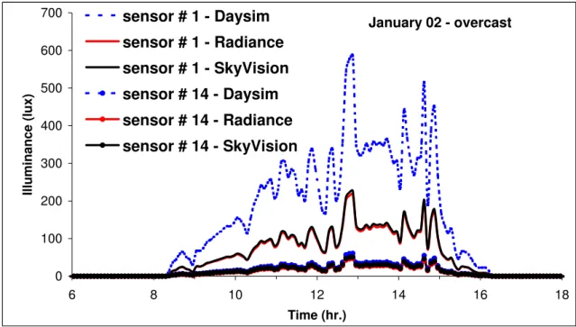
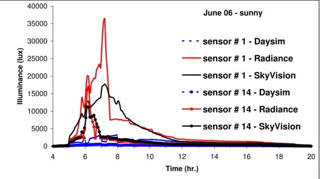
Figures 5 and 6 show a comparison of indoor illuminance at the front (#1) and back (#14) sensors as predicted using the optical models of Venetian blinds of the three programs: Daylight 1-2-3 (named “SkyVision”), "Radiance" and “Daysim” when the blinds are closed (slat angle = 45o down) during typical winter overcast and summer sunny days, respectively. The average sensor illuminances are also plotted in figure 7 for a typical summer sunny day. Under winter overcast days, the present model compares very well with Radiance. Daysim, however, produces indoor illuminances 165% higher than Radiance, particularly at the front sensor. This difference is due to the fact that the fixed diffuse blinds transmittance of 25% is significantly higher than the actual one, which is 5% (for sky light). Under summer sunny days, again the present model produces indoor illuminances very close to Radiance with a maximum difference less than 25%, particularly when sunbeam light hits the window during the morning hours. When the window is shaded from the sunbeam light during the afternoon hours, the present model overestimates indoor illuminance by up to 50% at

the back sensor (#14). The Daysim model underestimates the indoor illuminance by up to 60% during the morning hours, but produces comparable results during the afternoon hours. As for the average sensor illuminance (figure 7), the present model produces results very close to Radiance with a maximum difference less than 20% occurring during the afternoon hours. The model of Daysim still, however, underestimates illuminance by up to 60%, particularly during the morning hours.

0 100 200 300 400 500 600 700 6 8 10 12 14 16 18 Time (hr.) Illuminance (lux) sensor # 1 - Daysim sensor # 1 - Radiance sensor # 1 - SkyVision sensor # 14 - Daysim sensor # 14 - Radiance sensor # 14 - SkyVision January 02 - overcast

Figure 5 Indoor illuminance from an east-facing window under a winter overcast day: closed blinds– front (#1) and back (#14) sensors

0 500 1000 1500 2000 2500 3000 3500 4000 4 6 8 10 12 14 16 18 2 Time (hr.) Illuminance (lux) 0 sensor # 1 - Daysim sensor # 1 - Radiance sensor # 1 - SkyVision sensor # 14 - Daysim sensor # 14 - Radiance sensor # 14 - SkyVision June 06 - sunny

Figure 6 Indoor illuminance from an east-facing window under a summer sunny day: closed blinds– front (#1) and back (#14) sensors

0 200 400 600 800 1000 1200 1400 1600 1800 4 6 8 10 12 14 16 18 2 Time (hr.) Illuminance (lux) 0 Average - Daysim Average - Radiance Average - SkyVision June 06 - sunny

Figure 7 Sensor average illuminance from an east-facing window under a summer sunny day: closed blinds

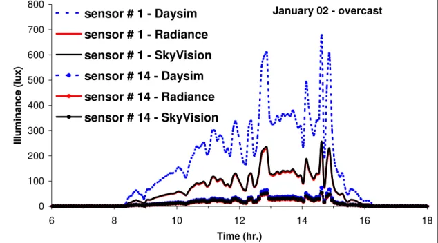
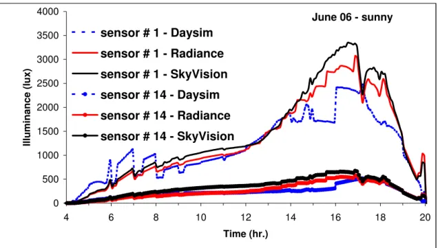
Figures 8 and 9 show a comparison of indoor illuminance at the front and back sensors when the blinds are open (slat angle = 0o) during typical winter overcast and

summer sunny days, respectively. The average sensor illuminances are also plotted in figure 10 for a typical summer sunny day. Under winter overcast days, the present model again compares very well with Radiance at all sensor positions. Daysim produces comparable results at the front sensors, but underestimates indoor illuminances by up to 60% at the back sensor when compared with Radiance. This is because Daysim uses a fixed blinds transmittance of 25%, which is significantly lower than the actual value when blinds are open. Under summer sunny days, the present model produces indoor illuminances 66% lower than Radiance when the sun shines on the window during the early morning hours (around 7:00 AM). When the window is shaded from sunlight during the late morning hours and on-wards (time > 8:00 AM), predictions from the present model are in good agreement with Radiance. The Daysim model greatly underestimates illuminance at all sensor positions, particularly during the morning hours (time < 12:00 PM). As for the average sensor illuminance (figure 10), the present model produces results close to Radiance with a maximum difference less than 25% occurring at illuminance peaks during the morning hours. The Daysim model underestimates the average illuminance by up to 95% during the morning hours. 0 100 200 300 400 500 600 700 6 8 10 12 14 16 18 Time (hr.) Illuminance (lux) sensor # 1 - Daysim sensor # 1 - Radiance sensor # 1 - SkyVision sensor # 14 - Daysim sensor # 14 - Radiance sensor # 14 - SkyVision January 02 - overcast

Figure 8 Indoor illuminance from an east-facing window under an overcast winter day: open blinds– front (#1) and back (#14) sensors

0 5000 10000 15000 20000 25000 30000 35000 40000 4 6 8 10 12 14 16 18 20 Time (hr.) Illuminance (lux) sensor # 1 - Daysim sensor # 1 - Radiance sensor # 1 - SkyVision sensor # 14 - Daysim sensor # 14 - Radiance sensor # 14 - SkyVision June 06 - sunny

Figure 9 Indoor illuminance from an east-facing window under a summer sunny day: open blinds– front (#1) and back (#14) sensors

0 2000 4000 6000 8000 10000 12000 14000 16000 18000 4 6 8 10 12 14 16 18 20 Time (hr.) Illuminance (lux) Average - Daysim Average - Radiance Average - SkyVision June 06 - sunny

Figure 10 Sensor average illuminance from an east-facing window under a summer sunny day: open blinds

West-Facing Window

Figures 11 and 12 show a comparison of indoor illuminance at the front and back sensors when the blinds are closed during typical winter overcast and summer sunny days, respectively. The average sensor illuminances are also plotted in figure 13 for

a typical summer sunny day. Under winter overcast days, the present model again compares very well with Radiance. Daysim, however, produces indoor illuminances 160% higher than Radiance, particularly at the front sensor. Under summer sunny days, the present model produces indoor illuminances close to Radiance at the front sensor with an error less than 20% occurring at the peak illuminance during the afternoon hours. It, however, overestimates illuminance by up 55% at the back sensor during the morning hours when the window is shaded from sunbeam light. The Daysim model underestimates indoor illuminance by up to 40% during the afternoon hours, but produces comparable results during morning hours. As for the average sensor illuminance (figure 13), the present model produces results very close to Radiance with a maximum difference less than 20% occurring during the morning hours. The model of Daysim still, however, underestimates illuminance by up to 40%, particularly during the afternoon hours.

0 100 200 300 400 500 600 700 800 6 8 10 12 14 16 18 Time (hr.) Illuminance (lux) sensor # 1 - Daysim sensor # 1 - Radiance sensor # 1 - SkyVision sensor # 14 - Daysim sensor # 14 - Radiance sensor # 14 - SkyVision January 02 - overcast

Figure 11 Indoor illuminance from a west-facing window under a winter overcast day: closed blinds– front (#1) and back (#14) sensors

0 500 1000 1500 2000 2500 3000 3500 4000 4 6 8 10 12 14 16 18 2 Time (hr.) Illuminance (lux) 0 sensor # 1 - Daysim sensor # 1 - Radiance sensor # 1 - SkyVision sensor # 14 - Daysim sensor # 14 - Radiance sensor # 14 - SkyVision June 06 - sunny

Figure 12 Indoor illuminance from a west-facing window under a summer sunny day: closed blinds– front (#1) and back (#14) sensors

0 200 400 600 800 1000 1200 1400 1600 4 6 8 10 12 14 16 18 2 Time (hr.) Illuminance (lux) 0 Average - Daysim Average - Radiance Average - SkyVision June 06 - sunny

Figure 13 Sensor average illuminance from a west-facing window under a summer sunny day: closed blinds

Figures 14 and 15 show a comparison of indoor illuminance at the front and back sensors when the blinds are open during typical winter overcast and summer sunny

days, respectively. The average sensor illuminances are also plotted in figure 16 for a typical summer sunny day. Under winter overcast days, the present model again compares very well with Radiance at all sensor positions. Daysim produces comparable results at the front sensor, but underestimates indoor illuminances by up to 60% at the back sensor when compared with Radiance. Under summer sunny days, the present model produces indoor illuminances lower than Radiance by up to 40% at the illuminance peaks when the sun shines on the window during the afternoon hours (around 5:00 PM). When the window is shaded from sunlight during the morning hours and early afternoon (time < 4:00 AM), predictions from the present model are in good agreement with Radiance. The Daysim model seems not suitable for illuminance prediction under sunny days as it greatly underestimates illuminance at all sensor positions, particularly during the afternoon hours. As for the average sensor illuminance (figure 16), the present model produces results close to Radiance with a maximum difference less than 25% occurring at the illuminance peaks during the afternoon hours. The model of Daysim underestimates the average illuminance by up to 95% during the afternoon hours.

0 100 200 300 400 500 600 700 800 6 8 10 12 14 16 18 Time (hr.) Illuminance (lux) sensor # 1 - Daysim sensor # 1 - Radiance sensor # 1 - SkyVision sensor # 14 - Daysim sensor # 14 - Radiance sensor # 14 - SkyVision January 02 - overcast

Figure 14 Indoor illuminance from a west-facing window under an overcast winter day: open blinds– front (#1) and back (#14) sensors

0 5000 10000 15000 20000 25000 4 6 8 10 12 14 16 18 20 Time (hr.) Illuminance (lux) sensor # 1 - Daysim sensor # 1 - Radiance sensor # 1 - SkyVision sensor # 14 - Daysim sensor # 14 - Radiance sensor # 14 - SkyVision June 06 - sunny

Figure 15 Indoor illuminance from a west-facing window under a summer sunny day: open blinds– front (#1) and back (#14) sensors

0 2000 4000 6000 8000 10000 12000 14000 4 6 8 10 12 14 16 18 20 Time (hr.) Illuminance (lux) Average - Daysim Average - Radiance Average - SkyVision June 06 - sunny

Figure 16 Sensor average illuminance from a west-facing window under a summer sunny day: open blinds

North-Facing Window

Figures 17 and 18 show a comparison of indoor illuminance at the front and back sensors when the blinds are closed during typical winter overcast and summer sunny days, respectively. The average sensor illuminances are also plotted in figure 19 for a typical summer sunny day. Under winter overcast days, the present model again compares very well with Radiance. Daysim, however, produces indoor illuminances 150% higher than Radiance, particularly at the front sensor. Under summer sunny days, the present model produces indoor illuminances close to Radiance at the front sensor with an error less than 15% occurring at noontime, but overestimates illuminance by up 60% at the back sensor. The Daysim model overestimates indoor illuminance at the front sensor by up to 150%, particularly during early morning or the afternoon hours when sunlight hits the window. Far from the window plane, the Daysim model provides comparable results to Radiance. As for the average sensor illuminance (figure 19), the present model produces results very close to Radiance with a maximum difference less than 20% occurring at noontime. The Daysim model also produces results close to Radiance with an error less than 25%.

0 100 200 300 400 500 600 6 8 10 12 14 16 18 Time (hr.) Illuminance (lux) sensor # 1 - Daysim sensor # 1 - Radiance sensor # 1 - SkyVision sensor # 14 - Daysim sensor # 14 - Radiance sensor # 14 - SkyVision January 02 - overcast

Figure 17 Indoor illuminance from a north-facing window under a winter overcast day: closed blinds– front (#1) and back (#14) sensors

0 500 1000 1500 2000 2500 4 6 8 10 12 14 16 18 2 Time (hr.) Illuminance (lux) 0 sensor # 1 - Daysim sensor # 1 - Radiance sensor # 1 - SkyVision sensor # 14 - Daysim sensor # 14 - Radiance sensor # 14 - SkyVision June 06 - sunny

Figure 18 Indoor illuminance from a north-facing window under a summer sunny day: closed blinds– front (#1) and back (#14) sensors

0 100 200 300 400 500 600 700 800 4 6 8 10 12 14 16 18 2 Time (hr.) Illuminance (lux) 0 Average - Daysim Average - Radiance Average - SkyVision June 06 - sunny

Figure 19 Sensor average illuminance from a north-facing window under a summer sunny day: closed blinds

Figures 20 and 21 show a comparison of indoor illuminance at the front and back sensors when the blinds are open during typical winter overcast and summer sunny days, respectively. The average sensor illuminances are also plotted in figure 22 for

a typical summer sunny day. Under winter overcast days, the present model again compares very well with Radiance at all sensor positions. Daysim produces comparable results at the front sensor, but underestimates indoor illuminances by up to 60% at the back sensor when compared with Radiance. Under summer sunny days, the present model produces indoor illuminances lower than Radiance by up to 30% occuring at noontime. The Daysim model underestimates illuminance at all sensor positions by up to 65%. As for the average sensor illuminance (figure 22), the present model produces results lower than Radiance by up to 25% occurring at noontime. The Daysim model also underestimates the average illuminance by up to 55%. 0 100 200 300 400 500 600 6 8 10 12 14 16 18 Time (hr.) Illuminance (lux) sensor # 1 - Daysim sensor # 1 - Radiance sensor # 1 - SkyVision sensor # 14 - Daysim sensor # 14 - Radiance sensor # 14 - SkyVision January 02 - overcast

Figure 20 Indoor illuminance from a north-facing window under an overcast winter day: open blinds– front (#1) and back (#14) sensors

0 500 1000 1500 2000 2500 3000 3500 4 6 8 10 12 14 16 18 2 Time (hr.) Illuminance (lux) 0 sensor # 1 - Daysim sensor # 1 - Radiance sensor # 1 - SkyVision sensor # 14 - Daysim sensor # 14 - Radiance sensor # 14 - SkyVision June 06 - sunny

Figure 21 Indoor illuminance from a north-facing window under a summer sunny day: open blinds– front (#1) and back (#14) sensors

0 200 400 600 800 1000 1200 4 6 8 10 12 14 16 18 2 Time (hr.) Illuminance (lux) 0 Average - Daysim Average - Radiance Average - SkyVision June 06 - sunny

Figure 22 Sensor average illuminance from a north-facing window under a summer sunny day: open blinds

DISCUSSION

In view of the comparison results between Radiance as a benchmark model and the present model, it was found that the present model yields accurate results under

overcast sky conditions for any blinds position and window orientation. When sunbeam light is dominant during sunny days, the present model results in some spatial illuminance discrepancies within the room space, particulary when blinds are open. However, the present model is in relatively good agreement with the benchmark model for the prediction of the average sensor illuminance (maximum error less than 25%). Two major causes may explain this discrepancy:

1. Light transmission through the blinds as modelled by Radiance is two dimensional (varies with height and width of window) as compared to the SkyVision model, which treats the blinds as a homogeneous layer. This means that if the distance between two consecutive blind slats is larger than the visual size of a point light source (such as the sun disk) the source image can be fully projected on particular points in a room, resuting in aletrnating bright and dark spots. The illuminance values of the bright spots will consequently increase substantially. This may explain the presence of illuminance peaks during sunny days when blinds are open (see figures 9 and 15). However, the spatial variation of illuminance may be smoothed out when light transmits through a homogeneous blind layer, resuting in gradual illuminance spatial variation rather than alternating bright and dark spots. To capture the effect of blind slat positions on point illuminance, a few sensors covering a larger area than the projected source image should be used. The latter may explain the good agreement between Radiance and the present model when the average sensor illuminances are compared. 2. Light scattering through the blinds system is not isotropic diffuse (as assumed in

SkyVision). Depending on the slat angle, light scattering may take the form of a narrow (when blinds are closed) or wide (when blinds are open) scattering. As a result of this scattering, sensors placed near the window may be illuminated by light inter-refection only. This explains why the illuminances as measured by the front sensor compared better than the illuminances measured by the back sensor when blinds are closed (see figure 6 during early afternoon hours, or figure 12 during late morning hours). When the blinds are open, the diffrence between both models is significantly reduced, supporting the argument that the wide scatter can be regarded as isotropic diffuse (see figure 9 during early afternoon hours, or figure 15 during late morning hours).

It should be added that the illuminance difference between the two models observed for the north-facing window may be attributed to both the effects of the point source size and blinds light scattering since the sky luminance exhibits high spacial variability during sunny days.

CONCLUSION

This paper presents a general methodology to compute daylight coefficient sets for rooms employing multiple dissimilar components of dynamic complex fenestration systems whose optical behaviour may change over time. DC set calculations may be performed prior to simulation start, resulting in substantial computational time saving for annual simulation. A validation study is carried out, in which daylight illuminances in an office space equipped with a clear window and internal Venetian blinds are compared using predictions from the present model as implemented in Daylight 1-2-3, Radiance, as a benchmark model employing detailed optical model of Venetian blinds, and Daysim employing a simple engineering blinds model.

The present model treats the room fenestration systems component by component. The DC set is calculated for each fenestration component, and the resulting room DC set is obtained by simple addition of component DC sets. With this component approach, provision for any optical changes of a fenestration component may be accounted for. Furthermore, any arithmetic operations (adding/subtracting a new fenestration component to existing system) or geometrical transformation (rotation of fenestration plane) may be performed on the component DC sets. To account for the optical changes of dynamic complex fenestration systems, an optical model based on splitting the transmittance and reflectance into two components – beam-beam and beam-diffuse – is adopted. Consequently the component DC set is split into two components: one beam-beam component for the beam-beam transmitted light and the second beam-diffuse component for the beam-diffuse transmitted light. Algorithms to compute these DC components are presented. The beam-beam component of DC depends on the daylight coefficient of a reference clear fenestration system and the beam-beam transmittance ratio of the actual and reference fenestration system. However, the beam-diffuse component of DC depends not only on the beam-diffuse transmittance ratio, but also on the average DC set of a hypothetical hemisphere surrounding the fenestration plane.

Findings from the validation study are that the present model yields accurate results for any window orientation under overcast sky conditions. Under sunny sky conditions, overall the present model compares well with the benchmark model, but with some local illuminance differences in areas under direct sunlight exposure. When the space average illuminances are compared, the present model yields better results with an error less than 25%. Results for the simple blinds model of Daysim show that the model is not accurate for daylighting simulation, particularly where sunlight is dominant.

ACKNOWLEDGMENT

The work was supported by the Panel on Energy Research and Development (PERD), Britsh Columbia Hydro, the National Research Council of Canada, and Natural Resources Canada. The authors are grateful for their contributions and continuous support to the project.

REFERENCES

Bourgeois D, Reinhart C F, Ward G. 2007. “A Standard Daylight Coefficient Model for Dynamic Daylighting Simulations”. Accepted for publication in Building Research & Information.

ISO. 2003. Standard ISO-15099. Thermal performance of windows, doors and shading devices - detailed calculations. International Standard Organisation; Geneva: Switzerland.

Laouadi, A. and Parekh, A. 2007. Optical model of complex fenestration systems. Lighting Research and Technology. 39(2): 123-145.

Laouadi A., Reinhart C., and Bourgeois D. 2007. Daylight coefficient and complex fenestration systems. Proc. of the 11th IBPSA Buildings Simulation Conference in Beijing, China.

Mardaljevic J. 2000a. “Simulation of annual daylighting profiles for internal illuminance”. Lighting Research and Technology. 32(2): 111-118.

Mardaljevic J. 2000b. Beyond Daylight Factors: An example study using daylight coefficients. Proc. CIBSE National Lighting Conference, York, UK, 2000, 177-186. NRC. 2006. SkyVision v1.2.1 National Research Council of Canada:

http://irc.nrc-cnrc.gc.ca/ie/lighting/daylight/skyvision_e.html

NRC. 2007. Daysim. National Research Council of Canada: www.daysim.com.

Reinhart C., Bourgeois D., Dubrous F., Laouadi A., Lopez P., and Stelescu O. 2007. Daylight 1-2-3 – a state-of-the-art daylighting/energy analysis software for initial design investigations. Proc. of the 11th IBPSA Buildings Simulation Conference in Beijing, China.

Reinhart C. F., Andersen M. 2006. “Development and validation of a Radiance model for a translucent panel. Energy & Buildings: 38(7):890-904.

Reinhart C. F., Walkenhorst O. 2001. “Dynamic Radiance-based Daylight Simulations for a full-scale Test Office with outer Venetian Blinds”. Energy & Buildings: 33(7):683-697.

Reinhart C., and Herkel S. 2000. The simulation of annual daylight illuminance distributions- a state of the art comparison of six RADIANCE-based methods. Energy & Buildings: 32:167-187.

Tregenza P.R. 1987. Subdivision of the sky hemisphere for luminance measurements. Lighting Research and Technology. 19, 13-14.

Tregenza P.R. and Waters I.M. 1983. “Daylight Coefficient”. Lighting Research and Technology. 15(2), 65-71.

Vartiainen E. 2000. Daylight Modeling and Optimization of Solar Facades. Ph.D. Thesis From the Faculty of Engineering Physics at the Helsinki University of Technology. http://lib.tkk.fi/Diss/2001/isbn9512253372/

Ward G, Shakespeare R. 1998. “Rendering with Radiance. The Art and Science of Lighting Visualization.” Morgan Kaufmann Publishers.