Publisher’s version / Version de l'éditeur:
BioMed Research International, 2015, pp. 1-18, 2015
READ THESE TERMS AND CONDITIONS CAREFULLY BEFORE USING THIS WEBSITE. https://nrc-publications.canada.ca/eng/copyright
Vous avez des questions? Nous pouvons vous aider. Pour communiquer directement avec un auteur, consultez la
première page de la revue dans laquelle son article a été publié afin de trouver ses coordonnées. Si vous n’arrivez pas à les repérer, communiquez avec nous à [email protected].
Questions? Contact the NRC Publications Archive team at
[email protected]. If you wish to email the authors directly, please see the first page of the publication for their contact information.
Archives des publications du CNRC
This publication could be one of several versions: author’s original, accepted manuscript or the publisher’s version. / La version de cette publication peut être l’une des suivantes : la version prépublication de l’auteur, la version acceptée du manuscrit ou la version de l’éditeur.
For the publisher’s version, please access the DOI link below./ Pour consulter la version de l’éditeur, utilisez le lien DOI ci-dessous.
https://doi.org/10.1155/2015/183918
Access and use of this website and the material on it are subject to the Terms and Conditions set forth at
Molecular dynamics, Monte Carlo simulations, and langevin dynamics:
a computational review
Paquet, Eric; Viktor, Herna L.
https://publications-cnrc.canada.ca/fra/droits
L’accès à ce site Web et l’utilisation de son contenu sont assujettis aux conditions présentées dans le site LISEZ CES CONDITIONS ATTENTIVEMENT AVANT D’UTILISER CE SITE WEB.
NRC Publications Record / Notice d'Archives des publications de CNRC:
https://nrc-publications.canada.ca/eng/view/object/?id=3d35879a-c4d3-4c24-a06c-7e67a97bf7df https://publications-cnrc.canada.ca/fra/voir/objet/?id=3d35879a-c4d3-4c24-a06c-7e67a97bf7dfReview Article
Molecular Dynamics, Monte Carlo Simulations,
and Langevin Dynamics: A Computational Review
Eric Paquet
1,2and Herna L. Viktor
21Vaccine Program, National Research Council, 1200 Montreal Road, Ottawa, ON, Canada K1A 0R6 2School of Electrical Engineering and Computer Science, University of Ottawa, 800 King Edward Road,
Ottawa, ON, Canada K1N 6N5
Correspondence should be addressed to Eric Paquet; [email protected] Received 28 August 2014; Accepted 5 November 2014
Academic Editor: Xuguang Li
Copyright © 2015 E. Paquet and H. L. Viktor. his is an open access article distributed under the Creative Commons Attribution License, which permits unrestricted use, distribution, and reproduction in any medium, provided the original work is properly cited.
Macromolecular structures, such as neuraminidases, hemagglutinins, and monoclonal antibodies, are not rigid entities. Rather, they are characterised by their lexibility, which is the result of the interaction and collective motion of their constituent atoms. his conformational diversity has a signiicant impact on their physicochemical and biological properties. Among these are their structural stability, the transport of ions through the M2 channel, drug resistance, macromolecular docking, binding energy, and rational epitope design. To assess these properties and to calculate the associated thermodynamical observables, the conformational space must be eiciently sampled and the dynamic of the constituent atoms must be simulated. his paper presents algorithms and techniques that address the abovementioned issues. To this end, a computational review of molecular dynamics, Monte Carlo simulations, Langevin dynamics, and free energy calculation is presented. he exposition is made from irst principles to promote a better understanding of the potentialities, limitations, applications, and interrelations of these computational methods.
1. Introduction
he ability to properly sample conigurational and confor-mational properties and to subsequently describe at the atomic level the dynamical evolution of complex macro-molecular systems has wide application. his research is of paramount importance in the study of macromolecu-lar stability of mutant proteins [1], molecular recognition, ions, and small molecule transportation of the inluenza M2 channel [2, 3], protein association, the role of protein lexibility for inluenza A RNA binding [4, 5], folding and hydration, inluenza neuraminidase inhibitor [6–9], drug resistance [10], enzymatic reactions, folding transitions [11,
12], screening [13], accessibility assessment (see Figure 1), and hemagglutinin fusion peptide [14]. One should also mention multivalent binding mode [15], docking [16], drug (e.g., Oseltamivir and Zanamivir) eiciency against mutants [17, 18], structural biochemistry [19], biophysics, molecu-lar biology, inluenza multiple dynamics interactions [20], enzymology, pharmaceutical chemistry [21], biotechnology, rational epitope design [22], computation vaccinology [23],
binding [24], and free energy [25,26]. For instance, one may wish to calculate the free energy to assess the strength and the stability of the bond in between a monoclonal antibody (mAb) and an antigen, such as the viral hemagglutinin, to quantify the eiciency of the neutralisation process.
his paper presents an algorithmic review from the irst principles of Monte Carlo simulation, molecular dynamics, and Langevin dynamics (i.e., techniques that have been shown to address the abovementioned scenario). We focus our attention on the algorithmic aspect, which, within the context of a review, has not received suicient attention. Our objective is not only to explain the algorithms but also to highlight their potential, limitations, applicability, interrelations, and generalisation in the context of molecular dynamics. To this end, a number of algorithmic approaches are presented in detail, and the pros and cons of each are highlighted. he algorithms are illustrated with examples related to the inluenza virus.
his paper is organised as follows. Monte Carlo simula-tions are reviewed inSection 2.Section 3is concerned with molecular dynamics in the microcanonical ensemble, that is, Volume 2015, Article ID 183918, 18 pages
Figure 1: Accessibility assessment of a region of the inluenza A virus (A/swine/Iowa/15/1930 (H1N1)).
at constant energy.Section 4extends molecular dynamics to the canonical and the isobaric-isothermal ensemble. Con-strained molecular dynamics, hybrid molecular dynamics, and steered molecular dynamics are also presented.Section 5
introduces Langevin and self-guided Langevin dynamics, and
Section 6is concerned with the calculation of the free energy.
he application of molecular dynamics to macromolecular docking is addressed inSection 7. Finally, the connection in between molecular dynamics and quantum mechanics (ab initio simulations) is outlined inSection 8. his is followed by a short conclusion.
2. Monte Carlo Simulations
he objective of a Monte Carlo (MC) simulation is to generate an ensemble of representative conigurations under speciic thermodynamics conditions for a complex macromolecular system [27]. Applying random perturbations to the sys-tem generates these conigurations. To properly sample the representative space, the perturbations must be suiciently large, energetically feasible and highly probable. Monte Carlo simulations do not provide information about time evolution. Rather, they provide an ensemble of representative conigu-rations, and, consequently, conformations from which prob-abilities and relevant thermodynamic observables, such as the free energy, may be calculated. Monte Carlo simulations are not only important on their own right, but they also play a fundamental role when designing complex and hybrid molecular dynamic (MD) algorithms [28].
his section is dedicated to Monte Carlo simulations.
In Section 2.1 we review some important notions about
Lagrangian and Hamiltonian dynamics, which are pervasive for both Monte Carlo simulations and molecular dynamics.
InSection 2.2 we introduce the partition function and the
probability density function, as well as the calculation of ther-modynamics observable associated with a macromolecule such as the hemagglutinin or the neuraminidase. he parti-tion funcparti-tion is instrumental in computing such observables.
InSection 2.3we explain how to eiciently sample the
repre-sentative space. For that, we introduce the notions of emission probability, transition probability, acceptance probability, and detailed balance.
Sampling is useful only when performed in realistic experimental conditions. For this reason we explain how to
sample in the canonical ensemble (with a constant number of particles, volume, and temperature) and also in the isothermal-isobaric ensemble (with a constant number of particles, pressure, and volume) in Sections 2.4 and 2.5, respectively. Finally, inSection 2.6we address the problem of sampling in the presence of numerous minima. his is a problem particularly acute when studying inluenza macromolecular structures such as the hemagglutinin and the neuraminidase.
2.1. Lagrangian and Hamiltonian Dynamics or How to For-mulate Our Problem. his section presents some important notions about Lagrangian and Hamiltonian dynamics, which are pervasive and recurrent for both MC and MD. Lagrangian and Hamiltonian dynamics provide an ideal framework for the description of complex macromolecular systems, both in Cartesian and generalised coordinates [29]. he Lagrangian is deined as the diference in between the kinetic and the potential energy:
L(�3�, ̇�3�) = K ( ̇�3�) − U (�3�) , (1) where the kinetic energy is given by
K= 3� ∑ �=1 1 2�� 2�̇� , (2)
and potential energy U(�3�) is a function of the posi-tions of the constituent atoms. he�3� are the generalised coordinates, and the 3�̇� are the generalised velocities. For instance, a generalised coordinate may be a bound length, a bound angle, or a dihedral angle. he space of all generalised coordinates and velocities is called the coniguration space. If one introduces the generalised momentum:
��≡ �� ̇�L
�, (3)
one may deine the Hamiltonian, which is the Legendre transformation of the Lagrangian:
H(�3�, �3�) = 3� ∑ �=1� �� �− L (�3�, ̇�3�(�3�, �3�)) . (4)
he Hamiltonian obeys the so-called Hamilton’s equations, which is just another formulation of Newton’s equations:
�H �� = 0; �̇� = � H ���; ̇��= −� H ���. (5)
hroughout the text, we will use both generalised and Cartesian coordinates: the Cartesian coordinates of the � constituent atom are noted r� ≡ [��, ��, ��]�. he set of all Cartesian coordinates is noted as
r�≡ r1, . . . , r�, (6) and the associated diferential volume element is expressed as �r�≡ �r1. . . �r�. (7)
In the next section, we introduce the notions of partition function and probability density function.
2.2. Partition Functions, Probability Density Functions, and Expectation or How to Compute Observables. Partition func-tions are pervasive to all Monte Carlo simulafunc-tions. hey are required to determine the number of microstates associated with a macromolecule, the probability of occurrence of a spe-ciic conformation, and the ensemble averages of observables, such as the enthalpy or thermodynamical quantities like the free energy from which the strength of a bound between a drug, such as Oseltamivir [30], and a viral neuraminidase may be asserted.
he number of microstates may be obtained by
Ω (�, �, �) ≡ �0�{�}∫ �p��r�� (H (r�, p�) − �) , (8)
where
�{�}= ℎ3�(�1
�!��! ⋅ ⋅ ⋅ ) (9)
is a quantum factor, which accounts for the indiscernibility of the various atomic species�, �, and so forth, ℎ is the Planck constant, and �(�) is Dirac delta function. he function Ω(�, �, �) counts the number of states of constant energy � in a system. It is directly related to the entropy
� (�, �, �) = ��ln٠(�, �, �) , (10) where��is the Boltzmann constant. he canonical partition function is deined as
� (�, �, �) ≡ ∫ �p��r�exp[−�H (r�, p�)] , (11)
where
� ≡ 1�
�� (12)
and � is the temperature. he canonical partition func-tion is a funcfunc-tional, which is uniquely determined by the Hamiltonian of the corresponding macromolecular system. If the indiscernibility factor is included in the deinition, the microcanonical partition function is noted as
� (�, �, �) ≡ �{�}� (�, �, �) . (13)
he probability that the macromolecule is in a state charac-terised by atomic positions r�, and atomic momenta p� is given by
Pr(r�, p�) �p��r�= exp[−�H (r
�, p�)] �p��r�
� (�, �, �) . (14) Consequently, the ensemble average of an observable� (such as the enthalpy) is obtained by weighting the various realisa-tions of the observable by their corresponding probability:
⟨�⟩ = ∫ �p��r�� (r�, p�) Pr (r�, p�) . (15)
he uncertainty (standard deviation) associated with the observable is given by
� (�) = √⟨�2⟩ − ⟨�⟩2. (16)
Unfortunately, it is not possible to integrate the partition function or to compute the probability directly. his is due to the large number of degrees of freedom. For instance, the Homo sapiens inluenza hemagglutinin is formed of approximately 23.000 atoms, which means that the partition function must be integrated in a 138.000-dimensional space. In the next section, we explain how to perform such integration eiciently.
2.3. Stochastic Sampling or How to Sample Eiciently hermo-dynamical Quantities. he multidimensional integrals asso-ciated with the probability and the partition function may be eiciently calculated with a procedure called Monte Carlo integration. In this approach the integration space is sampled according to a Markovian process and the integral is approximated by the average of the corresponding sampled states. Such an approach is eicient if the sampled states have a high probability of occurrence.
A suicient, but not necessary, condition for such an eicient sampling to hold is called detailed balance:
Pr(I) � (I �→ J) � (I �→ J)
= Pr (J) � (J �→ I) � (J �→ I) , (17) where Pr(I) is the probability (emission probability) that the system is in the state I ≡ {r�, p�}, �(I → J) is the transition probability from state I to state J, and�(I → J) is the acceptance probability of such a transition. If we assume that the transition probability is symmetrical
� (I �→ J) = � (J �→ I) , (18) then the detailed balance equation reduces to
� (I �→ J)
� (J �→ I) = PrPr(I) =(J) exp[−� (U (J) − U (I))] . (19) A possible solution for this equation is
� (I �→ J) = min {1, exp [−� (U (J) − U (I))]} . (20) his equation is the celebrated Metropolis algorithm [31]. Consequently, each state is deined from the previous one (Markovian process). A transition to a lower energy is always accepted, while a transition to a higher energy is accepted with probability exp[−�(U(J) − U(I))].
Numerous variations have been designed based on this algorithm [32,33]. For instance, the local elevation method enhances sampling by adding penalty potential to any state previously sampled (also known as a taboo search algorithm). Although useful, the microcanonical partition function is not realistic from an experimental point of view. Indeed, most observations are performed either at constant volume and temperature (canonical ensemble) or at constant pressure and temperature (isobaric-isothermal ensemble). hese distribu-tions are introduced in the next two secdistribu-tions.
2.4. Canonical Ensemble (NVT) Sampling or How to Sample in Realistic Experimental Conditions. he canonical ensemble is the ensemble associated with the observations made at constant volume and constant temperature. he conigura-tional canonical partition function associated with such an ensemble is obtained by marginalising the momenta in(11):
� (�, �, �) ≡ ∫ �r�exp[−�U (r�)] . (21)
It may also be deined as
� (�, �, �) ≡ �{�}� (�, �, �) , (22)
where the constant
�{�} = 1
(√ℎ2�/2���)3����! (√ℎ2�/2���)3����! ⋅ ⋅ ⋅
(23) takes into account the indiscernibility of the constituent atoms. Like in the microcanonical ensemble, the probability of occurrence of a given state{r�} is equal to
Pr���(r�) �r�= exp[−�U (r
�)] �r�
� (�, �, �) . (24) Consequently, the average value of an observable is given by
⟨�⟩ = � (�, �, �) ∫ �1 r�exp[−�U (r�)] � (r�) . (25) In the case of the canonical partition function, the acceptance probability associated with Monte Carlo method reduces to
����(r��→ r��)
= min {1, exp [−� (U (r��) − U (r�))]} . (26) From the canonical partition function, it is possible to obtain various thermodynamical quantities such as the Helmholtz free energy:
� (�, �, �) = −��� ln � (�, �, �) . (27)
Still, most observations are performed at constant pressure and temperature. To address this limitation, the isobaric-isothermal ensemble, as presented in the next section, is introduced.
2.5. Isobaric-Isothermal Ensemble (NPT) Sampling or How to Sample in Even More Realistic Experimental Conditions. he isobaric-isothermal ensemble is representative of many experimental conditions. From the microcanonical formal-ism, it is possible to demonstrate that the isobaric-isothermal conigurational partition function is equal to
� (�, �, �) ≡ ∫ �� exp [−���] ∫ �r�exp[−�U (r�)] . (28)
As usual, if the indiscernibility of the constituent atoms is taken into account, the partition function becomes
� (�, �, �) =��{�}
0 � (�, �, �) . (29)
Such a partition function assumes that the deformations of the macromolecular structure are isotropic (the same in all directions). hese deformations occur to maintain the pressure constant. If the deformations are anisotropic, the partition function must be modiied as follows:
� (�, �, �) = ∫ �H��(�, �, �, H) � (det H − �) , (30) where H is the tensor associated with an elementary paral-lelepiped volume, which must be integrated (marginalised) over all possible variations of the elementary shape. he probability that a macromolecular system is in a state r� is given by
Pr���(r�) �r�= exp[−���] exp [−�U (r
�)] �r�
� (�, �, �) . (31) Again, various thermodynamical quantities may be deined from the partition function such as the Gibbs free energy:
� (�, �, �) = −��� ln � (�, �, �) . (32)
he isobaric-isothermal acceptance probability associated with the Monte Carlo method is
����(r�, � �→ r��, ��)
= min {1, exp [−� (U (r��, ��) − U (r�, �))] × exp [−�� (��− �) + � ln �� ]} .�
(33)
Irrelevant of the ensemble in which the calculations are per-formed, the Metropolis algorithm may be impaired by local minima [27]. Indeed, the acceptance probability may become trapped in a local minimum of the potential energy, which may result in an inadequate sampling of the macromolecular states, as seen in the conformational states [32,33]. his issue is addressed in the following section.
2.6. Sampling and Local Minima or When Temperature May Help to Escape Local Minima. Many biomolecular processes associated with inluenza involve activated processes in which a high-energy barrier exists in between the initial and the inal state [34]. In order to eiciently sample the macromolecular states, this type of barrier must be overcome.
An eicient, although computationally expensive, approach to overcome such a barrier is called replica exchange (refer to [34] and, in the same spirit, [35]). hese methods involve a certain number of noninteracting simulations, called replicas, which are performed in parallel. Each simulation is characterised by its own temperature:
low temperature simulations tend to explore local minima, while high temperature simulations may overcome energy barriers and consequently move in between local minima. To favour a better exploration of the macromolecular states, the replicas are periodically exchanged (swapped) according to the following acceptance probability:
��(I �→ J)
= min {I, exp [− (�J− �I)
× (U (J)|�J− U (I)|�I)]} , (34) where �I≡ 1� ��I . (35)
his acceptance probability is similar to the ones introduced before, except for the fact that each state is characterised by its own temperature. Once the exchange is completed, the simulations resume normally until another exchange is performed. he whole procedure allows for a better sampling of the macromolecular states. For instance, this approach has been utilised recently, in conjunction with simulated annealing, for creating the infectious disease model of the H1N1 inluenza pandemic [36].
Until now, we have restricted ourselves to symmetri-cal transition functions. Oten, a better sampling may be obtained if a nonsymmetrical sampling function is employed. Let us consider the particular case in which the nonsymmet-rical function depends uniquely on the inal conformation:
� (I �→ J) = � (U (J)) . (36) hen, the acceptance probability becomes
� (I �→ J)
= min {1, � (� (U (J))U(I))exp[−� (U (J) − U (I))]} . (37) his is the so-called bias sampling algorithm [37], which con-siderably increases the conformational sampling eiciency of large macromolecular chains [38].
Although MC simulations allow us to sample the most probable macromolecular states, they do not provide us with their temporal evolution. he study of the temporal evolution of a macromolecular state is called molecular dynamics and is the subject of the next section.
3. Molecular Dynamics or When Time Matters
Molecular dynamics studies the temporal evolution of the coordinates and the momenta (the state) of a given macro-molecular structure. Such an evolution is called a trajectory. A typical trajectory is obtained by solving Newton’s equations. he trajectory is important in assessing numerous time-dependent observables [39] such as the accessibility of a given molecular surface [40], the interaction in between
a small molecule (e.g., a drug) and the hemagglutinin or the neuraminidase of a given inluenza strain, the interaction epitope-paratope in between an antigen (e.g., hemagglutinin) and an antibody (e.g., CR8020), the appearance and disap-pearance of a particular channel or cavity, and the fusion of the hemagglutinin with a cell membrane (fusion peptide), amongst others.
From an MD trajectory, it is possible to compute a tem-poral average of an observable by averaging this observable over time along the trajectory:
� = lim� → ∞1� ∫�
0��� (� (�) , ̇�(�)) . (38)
Although it has never been formally proven (and that it is not always applicable: for instance, when the trajectory is periodic or when the phase space is constituted of disconnected regions), the ergodicity principle is oten invoked [41]. he ergodicity principle states that the average over periods of time along a given trajectory of an observable is, at the limit, identical to the ensemble average of this observable as obtained, for instance, from Monte Carlo simulations:
� ≈ ⟨�⟩ . (39) As we will see later, ergodicity is instrumental in performing MD simulations in the canonical and isobaric-isothermal ensemble. he next section is devoted to the potential or force ield.
3.1. Potential or How to Approximate the Force Field. he choice of a proper potential is of the utmost importance in obtaining accurate molecular dynamics simulations [42]. he potential must be physically sound as well as computation-ally tractable. An approximate potential may be calculated from quantum mechanics and from the Born-Oppenheimer approximation in which only the positions of the atomic nucleus bonding are considered [42]. he potentials may be divided into bonding potentials and long-range potentials. he bonding potentials involve interaction with two atoms (bound lengths), three atoms (bound angles), and four atoms (dihedral angles). Long-range interactions are associated with the Lennard-Jones potential (van der Waal) and the Columbic potential. he harmonic approximation is utilised for the bonding potentials, which means that solely small displacements are accurately represented. he general form of the potential is U(r�) = ∑ ���(� − �0) 2+ ∑ � ��(� − �0) 2 + ∑ ���(� − �0) 2 + ∑ ���(1 + cos (�� − �))
+ ∑ ���(� − �0) 2 + ∑ �,����(( �0 �� ���) 12 − (� 0 �� ���) 6 +����� ����) , (40) where� is the bound length, � is the Urey-Bradley bound length,� is the bound angle, � is the dihedral angle, � is the improper dihedral angle,���is the distance in between atom� and�, ��,��,��,��, and��are constants,�0,�0,�0,�0, and�0�� are equilibrium positions,���is related to the Lennard-Jones well depth, and��is the efective dielectric constant. Finally, �� is the partial atomic charge associated with atom�: the
partial charge comes from the asymmetrical distribution of the electrons in the chemical bounds. he irst term on the last line is the van der Waal interaction (or Lennard-Jones potential), and the last term on the last line is the Columbic interaction. he parameters of the model are determined experimentally and from quantum mechanics. Among the most popular potentials are CHARMM and AMBER [42,43]. he two difer mostly in the manner in which the parameters are estimated. hese potentials may model proteins, lipids, ethers, and carbohydrates, as well as small molecules (e.g., drugs).
he number of interactions involved in long-range inter-actions rapidly becomes prohibitive. For instance, for the Columbic potential, there are potentially �!/2!(� − 2)! interactions, which correspond to approximately a quarter of billon interactions for an inluenza hemagglutinin. To reduce the computational burden, their action range is truncated. he truncation should be performed in such a way as not to introduce artiicial discontinuities, which may result in computational artefacts.
he next section is concerned with the reinement of experimentally determined macrostructures.
3.2. How to Minimize the Energy of the Conformation or How to Reine Experimentally Determined Structures. he position of the constituent atoms of a macromolecular structure is usually determined either through X-ray crystallography for the larger structure or through nuclear magnetic resonance (NMR) for the smaller molecules. If only the amino acid sequence is available, the three-dimensional structure may be inferred either from methods based on homology, such as threading, or from ab initio methods, which predict the structure from the sequence alone [44]. Among the larger structures associated with inluenza are the hemag-glutinin and the neuraminidase. Because a protein has to be crystallised to apply X-ray crystallography, the position of its constituent atoms may be distorted from their natural positions by the crystallisation process. Consequently, bond lengths and bond angles may be distorted and steric clashes in between atoms may occur. herefore, it is recommended to minimise the potential energy of the macromolecular structure to remediate this deiciency and to create a more realistic structure [45].
he global optimisation of nonlinear functions, such as the potential, is a notoriously diicult problem because of the complexity of the energy landscape and the profusion of local minima [46]. Usually, only local optimisation is performed. Such a minimisation may be achieved through various algorithms [46] such as the steepest descent algo-rithm, the conjugate gradient algoalgo-rithm, and the Newton-Raphson method. he irst two are based on the gradient, while the latter is based on the Hessian. In most cases a local optimisation is suicient to reine the structure.
If a global optimisation is suited or required, an approach such as simulated annealing must be utilised [47]. Simulated annealing is an MC method. he position of the atoms is subjected to small random displacements. he acceptance probability of such a displacement is given by
� (I �→ J)
= min {1, exp [−��(U (J)|��− U (I)|��)]} ,
(41)
where
��∈ {�1, . . . , ��} | ��+1< ��. (42)
his means that the temperature acts as a control parameter. Initially, the temperature is high, which implies that tran-sitions from lower to higher energy are allowed with non-negligible probability in being able to escape local minima. Subsequently, the temperature is gradually reduced (cooling) to decrease the occurrence of such a transition. Transitions to lower energy are always accepted. With a proper choice of temperatures, a global optimisation may be achieved. he position of the global minimum associated with the energy landscape may be further reined with local optimisation.
he next section is devoted to the solvation of macro-molecules.
3.3. Implicit and Explicit Solvation, Ions, and Poisson-Boltzmann Equation or How to Obtain Realistic Experimental Conditions. Macromolecules do not exist in isolation. Water molecules and ions surround them. Oten, to obtain a realistic simulation, the structure of interest must be solvated. Solvation is a vast and complex subject and we refer the reader to the literature for technical details [4,44, 45, 48]. his section is devoted to some aspects of solvation, which are particularly relevant to MD.
he solvation may be either implicit or explicit. In the case of an implicit solvation [11], the water molecules are replaced by a potential, which describe their average action while, in the case of an explicit solvation, the macromolecule is surrounded by a solvation box constituted of water molecules. It follows that computers have a limited amount of memory, and thus, the size of this box cannot be ininite. To reduce the number of water molecules, various shapes may be utilised such as cubic, rhombic, dodecahedron truncated octahedron, and sphere. he shape of the solvation box is chosen to minimise the number of molecules required for solvation while maintaining at all times a minimum bufer of solvent. Because of its inite dimensions, the solvation box presents
unnatural boundary efects, which should be minimised. his may be partially achieved with a larger solvation box or with periodic boundary conditions (PBC). For a rectangular solvation box, periodic boundary conditions are deined as
� (��) = � (��+ ��)�����=1,...,�,
� (��) = � (��+ ��)������=1,...,�,
� (��) = � (��+ ��)�����=1,...,�.
(43)
Much care must be taken when using periodic boundary conditions to avoid unphysical artefacts. For instance, if the boundary box is too small, the head of a macromolecule, such as the hemagglutinin, may interact with its own tail, which is extremely unrealistic. Also, if Columbic interactions are involved, the system must be electrostatically neutral; otherwise, the total charge becomes ininite due to the endless replication of the system associated with the PBC. Ions could be added to the solvation box to neutralise the system. Even if the latter is neutral, ions, such as sodium and chloride, may be added to reproduce the ionic strength of the solvent in which the macromolecule evolves. Due to the periodic nature of the boundary conditions, duplicate interactions may appear. It is customary to apply the minimum image convention in which such duplicate interactions are not allowed. If the structure is too large, the solvation may be limited to a speciic region of interest: for example, a binding site or a channel while implicit solvation may be utilised for the remaining part of the macromolecule. here are various solvation models [49–
52]. Generally, their parameters are adjusted to reproduce the enthalpy of vaporisation and density of water.
he solvation box increases the complexity of the simulation. Indeed, most of the computational efort is directed toward simulating the solvent. Nevertheless, dielec-tric screening, electrostatic efects, and free energy, among others, may only be simulated through explicit solvation, which, consequently, is amply justiied [53] though one should notice that explicit solvation does not allow for the simulation of the solvent viscosity.
If the macromolecule is solvated in an ionic solution, the electrostatic potential� may be obtained with a greater accuracy by solving the Poisson-Boltzmann equation:
� �r ⋅ (� (r) �� ( r) �r ) = −� (r) −∑� �=1��� ∞ � � (r) exp (−���� (r)) , (44)
where�(r) represents the charge density of the solute (the macromolecule),�� is the ionic charge,��∞is the ionic con-centration far from the solute,�(r) is the dielectric permittiv-ity, and�(r) is an accessibility factor. he Poisson-Boltzmann equation is oten used in modelling implicit solvation. It may be solved eiciently with inite element methods (FEM) [54]. In the next section, we show how to solve Newton’s equation to obtain the trajectory of a macromolecule.
3.4. Integration of Newton’s Equations: When Technical Details Matter. To obtain the trajectory associated with a given macromolecule, one should solve the corresponding New-ton’s equations. his is appropriate, since the trajectories are assumed to follow the laws of classical mechanics [55]. In this section we present a completely general approach from which most inite diference algorithms may be derived.
Newton’s equation and their generalisation, Hamilton’s equations, present two important characteristic: they are time-reversible and any ininitesimal volume in phase space (space of all coordinates and momenta) is conserved with time. he latter property is known as the Liouville theorem [56]:
�3�� (0) �3�� (0) = �3�� (�) �3�� (�) . (45)
his is another formulation of the conservation of the total energy of the system. Any numerical algorithm must enforce these two properties at all times to be physically realistic and consequently relevant. When aiming to derive a inite diferent algorithm that complies with these requirements, we start with the Liouville operator deined as
�� ≡ 3�∑ �=1[� H ������ � − � H ��� � ���] , (46)
where� = √−1. his operator allows recasting Hamilton’s equations in the form:
�3�(�) = exp [���] �3�(0) , (47)
which is known as the Liouville equation. In Cartesian coordinates the Liouville operator becomes
�� = ��1+ ��2, ��1≡ � ∑ �=1 p� �� ⋅ ��r�; ��2≡ � ∑ �=1(− �U (r�) �r� ) ⋅ ��p�. (48)
Because the two parts of the Liouville operator do not commute�1�2 ̸= �2�1, one must rely on the Trotter theorem [5] to develop the argument of the exponential:
exp[���]
= exp [� (�1+ �2) Δ�]
≈ exp [��2Δ�2 ]exp[��1Δ�] exp [��2Δ�2 ]
+ O (Δ�3) .
(49)
hen, if each exponential is approximated in terms of a truncated Taylor expansion, the Liouville equation becomes
r�(� + Δ�) = 2r�(�) − r�(� − Δ�) − 1� � �U (r�(�)) �r� Δ� 2+ O (Δ�4)����� ����� ��=1,...,� , (50)
which is the well-known Verlet algorithm [1]. Note that other common algorithms, such as the Leap Frog algorithm and the reference system propagator algorithm (RESPA), may be derived following a similar approach [6, 7]. he Liouville operator may be partitioned in more than one way. For instance, the potential may be divided into short- and long-range potentials (e.g., Coulombs and van der Waal). Since long-range potentials tend to change more slowly than short-range potentials, a larger time increment may be used for the former. If this procedure is repeated, a multiple time-step algorithm may be designed. Once the trajectory has been calculated, the functional important motions may be separated from the random thermal motion by performing a principal component analysis (PCA), which expresses the dominant modes as linear combinations of the underlying motion [57].
he algorithms described in this section are only valid when the total energy is conserved, that is, in the micro-canonical ensemble. In next section we show how to extend this approach to the experimentally more realistic canonical and isobaric-isothermal ensembles.
4. Non-Hamiltonian Molecular
Dynamics or How to Reproduce Realistic
Experimental Conditions during Molecular
Dynamics Simulations
To simulate realistic experimental conditions, the MD sim-ulations must be performed either at constant volume and temperature or at constant pressure and temperature. Unfor-tunately, the canonical and the isobaric-isothermal ensembles do not conserve the total energy. he conservation of a quantity, such as the volume or the pressure, requires a constant exchange of energy in between the macromolecular system and the surrounding heat bath. Such a process, in which the Liouville theorem is not valid, may be described in terms of non-Hamiltonian molecular dynamics [58], as will be detailed here. Firstly, we describe the general approach, which is subsequently applied to the canonical ensemble. 4.1. General Approach. To apply the abovementioned general method, we must complement the � Cartesian positions and momenta associated with the constituent atoms with� additional generalised coordinates and momenta. he set of all coordinates is collectively denoted by
� = [r�| p�| ��| ��
� ]�. (51)
It follows that the original Hamiltonian must be modiied to include the generalised coordinates as well as an adjustable parameterℓ:
H(r�, p�) �→ H�(r�, p�, ��, ��� ; ℓ) . (52) Unfortunately, the theory does not specify a particular form for the modiied Hamiltonian. Because of the non-Hamiltonian nature of the dynamics, the Liouville theorem does not apply, which means that elementary volume ele-ments are not conserved in phase space. he reason for this
is that the modiied dynamics have altered the geometry of the phase space from an Euclidean (lat) geometry to a Riemannian (curved) geometry. In Riemannian geometry, the Liouville theorem becomes [59]
√����detG(�(�))������(�) = √����detG(�(0))������(0), (53) where G(�) is the metric associated with the Riemannian space, and det is the determinant of the matrix. We are only interested in the determinant of this matrix since only the latter is involved in the microcanonical partition function associated with the non-Hamiltonian system. he latter may be obtained directly from
√����detG(�(�))���� = exp[−∫0��� (�) ⋅� ̇� (�) ��] . (54) he number of microstates associated with the non-Hamiltonian system may be written as
Ω (r�, p�, ��, �� � ; ℓ) = Ω0∫ ��√����detG(�)���� � ∏ �=1� (Λ�(�) − ��) , (55)
where ��√| det G(�)| is the invariant volume element in extended phase space andΛ�(�)−��is a function associated with a conservation law (for instance, the total energy, or the momentum associated with the barycentre of the system). If we integrate or marginalise the additional coordinates and momenta, we obtain a function that depends solely on the coordinates and momenta of the constituent atoms
Ω (r�, p�, ��, ��� ; ℓ) �������→∫ ������ �
Ω�(r�, p�; ℓ) . (56) he adjustable parameter is chosen in such a way that the marginalised microcanonical partition function is equal to the partition function of interest (for instance, the canonical (constant volume) partition function)
Ω (r�, p�, ��, ���; ℓ) �������→∫ ������
� Ω
�(r�, p�; ℓ) .
(57) In the next section, we further clarify these notions by applying the general approach to the canonical ensemble. 4.2. Molecular Dynamics at NVT. In this section we outline the method to obtain the Hamiltonian that describes the canonical ensemble. his Hamiltonian may be substituted in the Liouville operator to obtain a inite diference equation. he modiied Hamiltonian, called the Nos´e-Hoover chain Hamiltonian [29,60–62], is deined as HNHC= H (r�, p�) + � ∑ �=1 �2 �� 2��� + ℓ�1 � + � ∑ �=2 �� � , (58) where H(r�, p�) = �−1 ∑ �=1 ��2 � 2�� � + �2 ⊙ 2�⊙ + U (r ��) (59)
is the Hamiltonian of the macromolecule in barycentric coor-dinates, the primed variables are the barycentric coordinates (relative to the centre of mass), and⊙ refers to the barycentre. If we assume that the energy of the modiied Hamiltonian and the barycentre momentum are conserved (isolated system), we have, for the microcanonical partition function,
ΩNHC = Ω0∫ ���� ����p��−1��⊙�r��−1 × exp [(3� − 2) �1+ � ∑ �=2��] � (HNHC− �1) × � (��1� Ω− �2) . (60)
If we marginalise the additional coordinate and momenta and chooseℓ = 3�, the marginalised microcanonical partition function becomes equal to the canonical partition function, which means that the modiied Hamiltonian describes the dynamics of the canonical ensemble
Ω�(r�, p�)NHC�����ℓ=3�≡ � (�, �, �) . (61) In the next section we focus on the constrained molecular dynamics.
4.3. Constrained Molecular Dynamics or How to Reduce the Computational Complexity. Macromolecules, such as the inluenza hemagglutinin, possess many degrees of freedom. A typical inluenza hemagglutinin is constituted of approxi-mately 23.000 atoms, which means the macromolecules have typically 138.000 degrees of freedom in phase space (atomic positions and momenta). Unsurprisingly, the number of degrees of freedom increases dramatically if the structure is solvated. To reduce the computational complexity, it may be advantageous to impose constraints on certain degrees of freedom. Since the hydrogen atoms are light, they tend to follow the motion of heavier atoms quasi-instantaneously. Consequently, it is customary to ix their bonding length to reduce the computational burden. Let us assume that we have � holonomic (that depends only on time and coordinates) constraints:
��(�) = �����r�(�) − r�(�)�����2− �2�≡ 0. (62)
he constraints are enforced in the equations of motion with the method of Lagrange multipliers. Each constraint becomes a potential to which a variable is attached called a Lagrange multiplier��: �� ̈r�(�) = −�U (r �(�)) �r� + � ∑ �=1�� ��� �r� ����� ����� ��=1,...,� . (63) Since the constraints are holonomic, they must be enforced at all times:
��(� + Δ�) ≡ 0. (64)
If we perform a truncated Taylor development of the previous equation, we may demonstrate that such a condition remains valid if a correction is applied to the Lagrange multiplier at each time step:
̃��(� + Δ�) = ̃��(�) + �̃��, (65)
where ̃��(�) = (Δ�2/2)�� is the value of the Lagrange multiplier at time�, �̃�� is the correction, ̃��(� + Δ�) is the value of the Lagrange multiplier at time� + Δ�, and
A�̃� ≈ −� (r�(� + Δ�)) , (66) which are deined as
A= [A��] = [ � ∑ �=1 1 �� ���(r�(� + Δ�)) �r� ⋅ ���(r�(�)) �r� ] , �̃� = [�̃��] ; � = [��] . (67) In this the linear equation governing the corrections to the Lagrange multipliers in which r�(�) are the constrained atomic coordinates at time �. Consequently, to obtain the correction, one must solve the linear equation associated with the correction.
Algorithms distinguish themselves by the approach they use to solve this equation. For the RATTLE algorithm, this equation is solved analytically [63]. For the SHAKE algorithm [64], only the diagonal elements of the A matrix are considered to reduce the complexity of the calculation, while for the MSHAKE algorithm [65] the whole matrix is solved with the LU decomposition. If the constraints are periodical, they must be expressed in terms of quaternions in which case the algorithm becomes QSHAKE [66].
In the next section, we consider a hybrid approach based on both molecular dynamics and Monte Carlo simulations. 4.4. Hybrid Monte Carlo Dynamics or How to Wisely Accel-erate the Dynamics. In order to obtain realistic molecular dynamics simulations, the time increment must be kept small. Usually, the value of the time increment is chosen around 1 femtosecond (10−15 seconds), which is typically one to two orders of magnitude smaller than the time scale associated with the fastest molecular event, the bound-length vibration [48]. If one desires to explore slow molecular events, the time required to run the simulation may become rapidly prohibitive. For instance, the rotation of buried side chains takes about 10−4 to 1 second to complete, while an helix-coil transition may take as long as 104 seconds. he situation might be even worse with macromolecular docking. Naturally, the time increment could be increased but the corresponding trajectory becomes rapidly unphysical.
his problem may be partially solved with an approach called hybrid Monte Carlo (HMC) simulation [28, 67]. As indicated by its name, HMC is a combination of MD and MC. he time evolution of the macromolecule is calculated with standard MD but with larger time increments. he outcome
of a time iteration is accepted only if it is physically feasible. he feasibility of the outcome is assessed with a standard MC acceptance probability rule:
� (r�(�) , p�(�) �→ r�(� + Δ�) , p�(� + Δ�))
= min {1, exp [−� (H (r�(� + Δ�) , p�(� + Δ�))
− H (r�(�) , p�(�)))]} .
(68)
Note that there is an importance subtlety associated with HMC. Because Newton’s equations are time reversible (any trajectory may be reversed by inverting the direction of the motion), the transition probability must also be so [68]. hat implies that the transition probability must be chosen so that
� (r�(�) , p�(�) �→ r�(� + Δ�) , p�(� + Δ�))
= � (r�(� + Δ�) , −p�(� + Δ�) �→ r�(�) , −p�(�)) . (69) Otherwise, the HMC may generate unphysical results.
In the next section, we explore other ways that may be used to assess slow processes.
4.5. Computational Alchemy or How to Virtually Explore Experimentally Hidden Processes. Molecular dynamics is not limited to real physical potentials and equilibrium processes. Introducing an external, nonphysical, time-dependent, and possibly position-dependent potential may accelerate the dynamics of a slow process. his is called steered molecular dynamics or computational alchemy [69]. For instance, a force may be applied to a hemagglutinin to study potential conformational changes or to a drug (ligand) to analyse the docking process in between a drug and a neuraminidase. An example of how this could be achieved is by applying a random force (both in terms of amplitude and direction) to the barycentre of the ligand [70]. If the displacement of the ligand is above a certain threshold, the force is reapplied without modiication. Otherwise, a new random force is generated. he whole process is repeated until the desired outcome is obtained. Such an approach is oten combined with an immersive virtual environment to better visualise the outcome of the simulation [69]. In the next section, we explore an alternative to molecular dynamics and Monte Carlo simulations, namely, stochastic dynamics.
4.6. Molecular Dynamics and Inluenza. here have been numerous applications of molecular dynamics in studies related to the inluenza virus. For instance, molecular dynam-ics has been utilised for rational drug design for the inluenza neuraminidase [7]. It has been instrumental to illustrate that the electrostatic funnel directs binding of Tamilu to the inluenza N1 neuraminidase [8]. Using molecular dynamics, it has been revealed that HR1039 is a potent inhibitor of the 2009 A (H1N1) inluenza neuraminidase [9]. In addition, molecular dynamics has been valuable to show the role played by the BM2 channel in proton conductance and drug resistance for the inluenza virus B [10]. Using molecular
dynamics has made possible the design of inhibitor tar-geting drug-resistant mutants of the inluenza A virus M2. Finally, conformational analysis of peptides and lipids of the inluenza hemagglutinin fusion peptide in micelles and bilayer would not have been possible without the aid of molecular dynamics [14].
5. Langevin Dynamics, Self-Guide Langevin
Dynamics, and Self-Guided Molecular
Dynamics: Toward a Better Sampling of
the Conformational Space
he dynamics of a macromolecular system is entirely deter-mined by the potential U(r�) associated with the process. For computational and practical reasons, this potential is virtually always an approximation of the real physical potential. Stochastic (random) dynamics attempts to bridge the gap in between the real and the approximate potential. Stochastic dynamics does not attempt to deine the real potential but a general correction, which is independent on the particular details of the real potential. In other words, stochastic dynamics attempt to take into account the neglected degrees of freedom to obtain more realistic simulations, especially in the case of conformational sampling [71].
In this framework, it is assumed that each particle is under the inluence of the potential U(r�) and of a heat bath formed by the remaining� − 1 particles. Under general conditions using the Mori-Zwanzig theory [72] (one may obtain the same result by assuming that each particle is minimally coupled to a harmonic heat bath formed from the other particles), it is possible to demonstrate that the particles obey the generalised Langevin equation (GLE) [73]:
�� ̈r�(�) = −�U (r �(�)) �r� − ∫� 0�� ̇r�(�) ��(� − �) + ��(�)���������=1,...,�, (70)
where��(� − �) is the memory kernel or dynamic friction and
��(�) is a stochastic term with mean:
⟨��(�)⟩ = 0 (71)
and covariance:
⟨��(0) ��(�)⟩ = 2�������� (�) ���I. (72)
Consequently, the correction is formed of two terms: a friction term, which introduces an artiicial viscosity, and a stochastic term, which takes into account the unknown nature of the correction. One should notice that the frictional term depends on the previous history of the trajectory (Markovian process). he friction term is important in obtaining realistic simulations, as it takes into account the viscosity of the solvent (a feature, which is absent from both MD and MC). If one assumes that the frictional term is
constant (no history), one obtains the celebrated Langevin equation (LE): ̇p�(�) = −�U (r �(�)) �r� − �� ̇p�(�) + ��(�) ����� ����� ��=1,...,� . (73) In that particular case,�� is simply called the frictional or damping term. he Langevin equation improves conforma-tional sampling over standard molecular dynamics.
Conformational sampling may still be further improved if the trajectory history is reintroduced into the model [71]. To take history into account, a history-dependent guiding term
Γ�(�) is added to the Langevin equation: ̇p�(�) = −�U (r �(�)) �r� − �� ̇p�(�) + ��(�) + ��Γ�(�) ����� ����� ��=1,...,� . (74) his term could be deined in various manners. In self-guided Langevin dynamics (SGLD), the history-dependent guiding term is deined as the time average of the momentum over the lastℓ iterations:
SGLD�(�)
= ��p�(�)������∈[�−ℓΔ�,�]
= (1 − Δ�ℓΔ�) Γ�(� − Δ�) + Δ�ℓΔ����� ̇r�(� − Δ�2 ) .
(75)
When, for self-guided molecular dynamics (SGMD), the history-dependent guiding term is deined as the time aver-age of the potential plus its self-time averaver-age,
SGMDΓ�(�) = −�U (r�r�(�)) � + ��Γ�(�) ����� ����� ���∈[�−ℓΔ�,�] = (1 − Δ�ℓΔ�) Γ�(� − Δ�) + Δ�ℓΔ� (−�U (r�r�(�)) � + ��Γ�(�)) . (76)
he guiding term is unphysical (as opposed to the memory kernel) and does not conserve energy. To reestablish energy conservation, an additional term �(�)p�(�), proportional to the momentum, must be added to the SGLD equation:
̇p�(�) = −�U (r
�(�))
�r� − �� ̇p�(�)
+ ��(�) + ��Γ�(�) − � (�) p�(�)�����=1,...,�.
(77)
his term ensures the conservation of energy, providing that the running constant�(�) obeys
� (�) = ∑��=1��Γ�(�) ⋅ ̇r�(�)
∑��=1p�(�) ⋅ ̇r�(�) .
(78)
hese equations may be easily integrated if they are recast under the form of Wiener processes [74]. he integration requires two independent Gaussian random variables.
Langevin dynamics has been used in many applications. For instance it has been instrumental to unravel the bilayer conformation of the fusion peptide of the inluenza virus hemagglutinin [75]. Further, the use of Langevin dynamics aided researchers to characterise the loop dynamics and ligand recognition in human- and avian-type inluenza neu-raminidase [76].
In the next section, we address complexes stability such as an interaction between a drug and neuraminidase or that between monoclonal antibodies and hemagglutinin.
6. Free Energy, Binding, and Complexes or
a Measure of Stability
he interaction in between a small molecule (drug) or an antibody with an antigen (hemagglutinin or neuraminidase) may result in a complex. It follows that, oten, the stability of such a complex must be assessed. Indeed, if the complex is stable, the small molecule or the antibody may eiciently neutralise the corresponding antigen. Free energy [53] is a measure of such stability. Consequently, the calculation of free energy is addressed in the next section.
6.1. hermodynamic Integration. he thermodynamics inte-gration method [77] requires two states to determine the free energy: an unbound state I and a bound state J. From them, a parametric potential is deined as a linear superposition of the two potentials:
U(r�; �) = (1 − �) UI(r�) + �UJ(r�) . (79) A corresponding parametric partition function is also deined as follows:
� (�, �, �; �) = ∫ �r�exp[−�U (r�; �)] . (80) Such a procedure is called adiabatic switching. he paramet-ric derivative of the free energy may be obtained from the deinition of the free energy:
�� (�, �, �; �)
�� = − 1���� ln� (�, �, �; �) . (81) It follows that the diference of free energy in between the bound and the unbound state may be evaluated from
�J− �I= ∫ 1 0 �� ⟨ �U (r�; �) �� ⟩U(r�;�). (82) In the next section, we introduce a method based on irre-versible work.
6.2. Nonequilibrium Method. In this section we describe an approach inspired from steered molecular dynamics
the nonequilibrium method does not require the bound state. his state is reached as a result of the irreversible work efectuated by the synthetic time-dependent Hamiltonian. he nonequilibrium method is based on Jarzinski’s equality and irreversible work [78]. Jarzinski’s equality may be derived from a time-dependent Hamiltonian ensemble average and the Liouville theorem. From this equality, the diference in free energy in between a bound and an unbound state may be calculated from the ensemble average of the irreversible work applied to the system to bring the unbound state into a bound state:
�J− �I = −�� ln ⟨exp [−�WIJ(r�, p�)]⟩I, (83)
where WIJ(r�, p�), the irreversible work, is given by
WIJ(r�, p�) = ∫ �J
�I ��
�HIJ(r�, p�, �)
�� , (84) and where the time-dependent Hamiltonian HIJ(r�, p�, �)
is equal to the sum of the unbound macromolecular Hamil-tonian HI(r�, p�) and of an external arbitrary
time-dependent potential UIJ(r�; �), which brings the
macro-molecular system from an unbound state I to a bound state J:
HIJ(r�, p�, �) = HI(r�, p�) + UIJ(r�; �) . (85) he ensemble average of the irreversible work is performed with the unbound Hamiltonian:
⟨exp [−�WIJ(r�, p�)]⟩I = (∫ �p��r�exp[−�WIJ(r�, p�)] × exp [−�HI(r�, p�)]) × (�I(�, �, �)) −1. (86)
he next two sections present methods, which evaluate the free energy based on a subset of their generalised coordinates.
6.3. Blue Moon Ensemble Approach. hermodynamic inte-gration and the nonequilibrium method both exploit all the coordinates and momenta associated with the macromolec-ular system to evaluate the free energy. Correspondingly, one may evaluate the free energy from a subset called the reaction coordinates (e.g., bound length and bound angle) of the generalised coordinates such as the generalised coordinates directly associated with the binding process. his consider-ably reduces the complexity of the calculation but introduces a certain level of approximation, as most coordinates are neglected. In order not to clutter the notation, we will use only one reaction coordinate while keeping in mind that the generalisation of more than one coordinates is immediate.
he probability that a reaction coordinate��has a value � is Pr(�) =∫ �p ��r�exp[−�H] � (� �(r�) − �) � (�, �, �) , (87) where ��= ��(r�) (88)
is the representation of the reaction coordinates in terms of the Cartesian coordinates. he free energy associated with this coordinate is by deinition
� (�) = −���lnPr (�) . (89) If we marginalise (integrate) the momenta and if we express the potential in terms of the generalised coordinates, we obtain for the free energy [79]
� (�) = � (��) + ∫� ��⟨ �U (r�(�3�)) ��� − ���� ln det J ��� ⟩���, (90) where ⟨�⟩�= � (�, �, �) ⟨� (�1 �− �)⟩ × ∫ ��3�� × exp [−� (U (r�(�3�)) − ���ln det J)] � (��− �) , (91)
and where the Jacobian matrix of the transformation is
J= �r
�
��3�. (92)
he main disadvantage of this approach is that all Cartesian coordinates must be converted into generalised coordinates, although only a subset of them (the reactions coordinates) are efectively exploited in the calculation of the free energy. his ineiciency is addressed in the next section.
6.4. Umbrella Sampling and Weighted Histogram Methods. When using umbrella sampling [80,81] and the weighted his-togram method [82] for the blue moon ensemble approach, the free energy is estimated from the reaction coordinates. he range (codomain and image) associated with the reaction coordinates is divided into a set of windows or intervals. A reaction coordinate distribution is associated with each win-dow. he unbiased estimator for the probability of occurrence of a reaction coordinate within a given window is assumed to be the product of a biased Gaussian probability distribution and a biased correction based on an umbrella potential:
Pr(�) ≈ 1 √2��2 � exp[−(� − ��) 2 2�2 � ] exp [−�� (�, � (�))] , (93)
where
� (�, �(�)) = 12�(� − �(�))2 (94) is the harmonic umbrella potential and �(�) is the centre of a given window, while �� and �2� are, respectively, the average and the variance of all the realisations of the reaction coordinates within window�. By deinition, the derivative of the free energy associated with a particular window is equal to ��� �� = −Pr��(�)� � Pr (�) �� =���2� � (� − ��) − � (� − � (�)) . (95) It is assumed that the derivative of the total free energy is a combination of the derivatives of the windows’ free energy:
�� �� = � ∑ �=1��(�) �� � �� , (96)
and that the weighting coeicients are normalised
�
∑
�=1��(�) = 1.
(97) he full free energy proile may be extracted with numerical integration. In the next section, we describe another approach for the calculation of the free energy, which introduces a bias potential to better sample the reaction coordinates.
6.5. Metadynamics. As opposed to the previous methods, which were based on a single molecular dynamics simulation, the metadynamics approach involved two molecular dynam-ics simulations: the usual one in Cartesian coordinates under the inluence of the real physical potential and a second one, the meta-simulation, which is performed under the inluence of a biased potential. he bias potential is deined as
U�(r�) = � ∑ �=��,2��,... exp [ [− � ∑ �=1 (��(r�(�)) − ��(r��(�)))2 2Δ�2 ] ], (98) where � is a constant, �� is a time interval; r�(�) is the time evolution (trajectory) of the complete set of Cartesian coordinates up to time� under the action of the real physical potential U(r�), and r��(�) is the trajectory of the system under the inluence of both the physical potential and the biased potential U(r�) + U�(r�). From an analysis based on the Langevin equation, it is possible to demonstrate that the free energy may be obtained from
� (��) ≈ � ∑ �=��,2��,...exp [[− � ∑ �=1 (��− ��(r��(�)))2 2Δ�2 ] ], (99)
in which the reaction coordinates are expressed in a function of the metacoordinates. he proof of this equation is beyond the scope of this review and may be found in [83]. As for umbrella sampling, only the reaction coordinates need to be expressed in terms of the Cartesian coordinates.
he use of free energy calculations has provided insights into the susceptibility of antiviral drugs against the E119G mutant of the 2009 inluenza A (H1N1) neuraminidase [26]. It has also been utilized to show the impact of calcium on the N1 inluenza neuraminidase [25].
In the next section, we explain how molecular dynamics may be combined with macromolecular docking to assert the dynamics of a macromolecular complex, such as a viral hemagglutinin, when interacting with a broadly neutralizing monoclonal antibody.
7. Binding and Docking or Computational
Pharmacology and Vaccinology
From the outset, one may assume that the relative pose of the constituent of a complex may be obtained through molecular dynamics without resorting to macromolecular docking. Although this is, in principle, feasible, it is usually not realistic in practice. Indeed, the time scale associated with macromolecular docking is usually out of reach for most molecular dynamics simulations [48]. Larger time steps may be taken if a hybrid Monte Carlo approach is followed
(Section 4.4), but most of the time, the increase is
insui-cient. For this reason macromolecular docking remains the favourite method to determine the relative pose in between a receptor and a ligand. (Note that macromolecular docking is beyond the scope of this paper, but a comprehensive algorithmic review may be found in [84]).
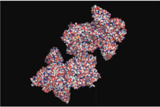
he abovementioned observation does not imply that MD is irrelevant for macromolecular docking. On the con-trary, once the pose in between the receptor and the ligand has been determined through macromolecular docking, the dynamics of the resulting complex may be explored with MD simulations. Various dynamical aspects of the complex may be studied. hese include the study of the conformational space associated with the receptor [85], binding path anal-ysis [56], examining the structural changes associated with induced it, studying the lexibility of the docking region, analysing transient binding, and aiding in structural reine-ment of the complex [86] as well as the design of drugs [87] and antibodies (seeFigure 2) with optimal kinetic properties. MD may also be employed prior to macromolecular docking to generate conformations, which become the initial point for static docking. his is particularly beneicial if the ligand binds to conformations that rarely occur (relax complex method). Nevertheless, standard MD should not be utilised to explore low frequency motions associated with large conformational transformations. his is due to its limited ability to explore conformational change. Langevin dynamics may be more suited in that particular case. Also, from a computational point of view, multiple copies of the ligand may simultaneously interact with the receptor to search, in parallel, for the best docking region. here should be no
Figure 2: Molecular surface of inluenza hemagglutinin (A/Viet Nam/1203/2004 (H5N1)) in complex with a broadly neutralizing antibody F10.
interaction in between the copies. Molecular dynamics may also be utilised to evaluate the structural accessibility of a highly conserved epitope [4].
In the next section, we briely explore the relationship in between quantum mechanics and molecular dynamics.
8. Path Integral or When Quantum Mechanics
Meets Molecular Dynamics
he calculations that we have performed so far are based on classical and semiclassical approximations of quantum mechanics. hough being valid, these approximations are not as accurate as their quantum-mechanical counterpart [88]. However, quantum-mechanical (QM) methods are oten computationally prohibitive. For that reason, quantum-mechanical methods are restricted to a small number of coordinates of interest (reaction coordinates) and the residual coordinates are analysed with molecular dynamics (the so-called hybrid quantum-mechanical molecular dynamics). Quantum mechanical methods are outside the scope of this review. More details may be found in [88]. Here, we limit ourselves to the connection in between quantum-mechanical methods and molecular dynamics. Quantum-mechanical methods are also based on the partition function formalism, which in the quantum case takes the form:
� (�, �, �) = tr exp [−�̂H] , (100) where tr is the trace operator and ̂His the quantum Hamil-tonian operator, which may be obtained from the classical Hamiltonian as follows:
H(r�, ℏ� �
�r�) �→ ̂H. (101)
By extensively using the following identities: ∫ �� |�⟩ ⟨�| = ̂�; ∫ �� �����⟩⟨����� = ̂�;
⟨� | �⟩ = exp [ℏ���],
(102)
and by making a certain number of approximations (Born-Oppenheimer approximation, Boltzmann statistics, and adi-abatic approximation [83], etc.), it may be demonstrated that the partition function
� (�, �, �) = ∮ Dr1(�) ⋅ ⋅ ⋅ Dr�(�) × exp [−1ℎ ∫0�ℎ��12 � ∑ �=1�� ̇r 2 �(�) + U (r�(�))] (103)
is equal to the path integral over all possible closed paths of the exponential of the classical Hamiltonian. he notation Dr�(�) means that we must integrate r�(�) over all possible
paths or trajectories. he resulting approach is known as path integral molecular dynamics [89]. Equation (103) involves only the atomics coordinates, but it is possible to introduce the conjugate momenta without altering the partition func-tion by adding a harmonic potential to the Hamiltonian:
� (�, �, �) = ∮ Dr1(�) ⋅ ⋅ ⋅ Dr�(�) Dp1(�) Dp�(�) × exp [−1ℎ ∫0�ℎ�� � ∑ �=1 p2� 2�� � (�)] × exp [−1ℎ ∫0�ℎ � ∑ �=1 1 2����2r2�(�) + U (r�(�))] , (104) where �� � = �(2�ℎ)��2; ��=√��ℎ ; � �→ ∞. (105)
he two equations are entirely equivalent. If we develop the notation, we obtain � (�, �, �) ≈ ∫∏� �=1�r (1) � ⋅ ⋅ ⋅ �r(�)� �p(1)� ⋅ ⋅ ⋅ �p(�)� × exp [−�∑� �=1 � ∑ �=1 (p(�)� )2 2�� � + 12��� 2 �(r(�+1)� − r(�)� )2 + 1�U(r(�) 1 ⋅ ⋅ ⋅ r(�)�)]���������� r(�+1) � =r(1)� ∀� . (106)