Publisher’s version / Version de l'éditeur:
Thermochimica Acta, 436, October, pp. 35-42, 2005-10-01
READ THESE TERMS AND CONDITIONS CAREFULLY BEFORE USING THIS WEBSITE.
https://nrc-publications.canada.ca/eng/copyright
Vous avez des questions? Nous pouvons vous aider. Pour communiquer directement avec un auteur, consultez la
première page de la revue dans laquelle son article a été publié afin de trouver ses coordonnées. Si vous n’arrivez pas à les repérer, communiquez avec nous à PublicationsArchive-ArchivesPublications@nrc-cnrc.gc.ca.
Questions? Contact the NRC Publications Archive team at
PublicationsArchive-ArchivesPublications@nrc-cnrc.gc.ca. If you wish to email the authors directly, please see the first page of the publication for their contact information.
NRC Publications Archive
Archives des publications du CNRC
This publication could be one of several versions: author’s original, accepted manuscript or the publisher’s version. / La version de cette publication peut être l’une des suivantes : la version prépublication de l’auteur, la version acceptée du manuscrit ou la version de l’éditeur.
For the publisher’s version, please access the DOI link below./ Pour consulter la version de l’éditeur, utilisez le lien DOI ci-dessous.
https://doi.org/10.1016/j.tca.2005.06.025
Access and use of this website and the material on it are subject to the Terms and Conditions set forth at
Solventless fingerprinting of bituminous materials: a high-resolution thermogravimetric method
Masson, J-F.; Bundalo-Perc, S.
https://publications-cnrc.canada.ca/fra/droits
L’accès à ce site Web et l’utilisation de son contenu sont assujettis aux conditions présentées dans le site LISEZ CES CONDITIONS ATTENTIVEMENT AVANT D’UTILISER CE SITE WEB.
NRC Publications Record / Notice d'Archives des publications de CNRC:
https://nrc-publications.canada.ca/eng/view/object/?id=1c3ef008-8345-480b-978b-3dcb9d850263 https://publications-cnrc.canada.ca/fra/voir/objet/?id=1c3ef008-8345-480b-978b-3dcb9d850263
Solventless fingerprinting of bituminous materials: a high-resolution thermogravimetric method
Masson, J-F., Bundalo-Perc, S.
NRCC-47735
A version of this document is published in / Une version de ce document se trouve dans: Thermochimica Acta, v. 436, nos. 1-2, Oct. 2005, pp. 35-42
Doi: 10.1016/j.tca.2005.06.025
Solventless Fingerprinting of Bituminous Materials: A High-Resolution Thermogravimetric Method
J-F. Masson* and Slađana Bundalo-Perc
Institute for Research in Construction, National Research Council of Canada Ottawa, Ontario, Canada, K1A 0R6
*Corresponding author. Phone: (613) 993-2144. Fax (613) 952-8102. e-mail: jean-francois.masson@nrc.gc.ca
Abstract
The thermogravimetric analysis (TGA) of bituminous materials by means of a constant heat rate is often plagued by low resolution and poor reproducibility of the degradation or mass loss temperatures. The TGA curve, or the associated differential TGA (DTGA) signal, is thus an unreliable quality control or quality assurance (QC/QA) method. A 2- and 3-step high-resolution TGA/DTGA method was developed for these materials for analysis between 150°C and 800°C. The DTGA results, obtained within 2h, show about ten discrete mass peaks, the profile being material dependant. The reproducibility of the results indicate that the methods may be used for rapid QC/QA and material fingerprinting. The development of the method is detailed and its application is illustrated with the analysis of several bitumens and polymer-modified bituminous sealants.
1. Introduction
Bitumen is the basis of products that find numerous applications in civil engineering, including water-based coatings, roadway binders, and polymer-modified bituminous waterproofing membranes and sealants. For the industrial production of materials with consistent properties, it is often desirable to use raw materials of a constant composition or grade. Products of identical grades can have different compositions [1], however, as indicated in Table 1. A constant chemical composition may be required for some applications, an important one being the production of stable bitumen-polymer mixtures [2].
The composition of bitumen is often controlled by means of chromatography (for various methods see Table 1 in [3]). This approach requires the separation of bitumen into several fractions. The composition as indicated in Table 1, for instance, is unique and serves to control the identity of a raw material. It is a fingerprint tedious to obtain, however, and it requires that several organic solvents be used and later discarded.
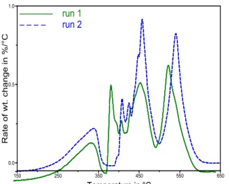
In contrast to chromatography, thermogravimetric analysis (TGA)/differential TGA (DTGA) is a solventless method. In standard TGA, a sample is heated at a constant rate. The method, which provides information about thermal stability and weight loss with rising temperature, has long been used to characterize petroleum products [4, 5]. Despite some success, the method shows poor resolution and reproducibility, especially in the 350-450°C region, where uncontrolled combustion (auto-ignition) occurs [6]. Fig. 1 shows an example with bitumen duplicates. Due to poor reproducibility, the DTGA profile has not permitted successful fingerprinting of bitumen [7]. Alternative methods used to overcome this difficulty have consisted of the measurement of weight loss at
fixed temperatures, e.g. 2 min at 350°C, 500°C and 750°C [8], and the quantification of the heaviest bitumen fraction after heating at rapid rates [9].
In this paper, it is shown that a 3-step high-resolution TGA/DTGA method can be used to improve both the resolution and the reproducibility of the results to a level that allows for rapid QC/QA and true fingerprinting of bituminous products at all temperatures between 150°C and 800°C. Fig. 2 shows an example of the type of
improvement that can be obtained. The aim of this paper is to show how such improvements were made possible and to describe some applications of the method by showing results for bitumens and bituminous sealants. It is best, however, to begin with a brief review of the basis for TGA/DTGA where samples are not heated at a constant rate. To be concise, the following abbreviations are used: dp/dt, rate of pressure change; dm/dt, rate of mass loss; dT/dt, heat rate; dT/dt(max), maximum heat rate; dT/dt(min), minimum heat rate; R, resolution setting; and S, sensitivity setting.
2. Varying rate TGA/DTGA
2.1 Early methods
To increase the resolution of TGA over what is possible with a linear rate of heating, Rouquerol [10, 11] and Paulik and Paulik [12, 13] independently developed the idea of using the thermal characteristics of the sample to control its heat rate and achieve quasi-equilibrium conditions. Under such conditions, a pre-determined temperature program no longer exists. Methods based on this guiding principle have received close to twenty names over time [11]. In the current state of the technology, the thermal characteristics are not limited to mass, but also include length, heat flow and evolved gas flow [11]. In TGA, the sample mass is monitored.
To achieve a non-linear heat rate, Rouquerol [10] evacuated a sample bulb linked to a pressure gauge connected to a temperature controller. As the sample was heated and the vapour pressure increased, the heating was reduced. The effect was thermal decomposition at a constant rate. With the use of an electro-balance and feedback loop, Paulik and Paulik [12] demonstrated that a linear heat rate (0.5-5°C/min) could be reduced when a weight loss was detected. The result was a very slow heat rate, i.e. quasi-isothermal conditions, that led to sample decomposition rates in the range of 0.1 to 0.5 %/min [13].
Rouquerol and the Pauliks obtained very slow heat rates by measuring dp/dt and dm/dt, respectively. In such quasi-equilibrium conditions, sample decomposition occurs within a narrow temperature interval, which improves resolution. Sorensen later developed a similar control [14], whereupon a sample was heated at a constant rate until a predetermined rate of mass change was detected. The isotherm was then held until the mass loss rate dropped below another predetermined threshold. This approach, useful for measuring decomposition kinetics, is known as stepwise isothermal analysis [15, 16].
2.2 Control algorithms
The increase in resolution that follows a reduced rate of heating comes at the expense of experimental time. To shorten experimental times while maintaining high resolution, Crowe and Sauerbrunn developed algorithms [17, 18] that, amongst other things, allow for very high heat rates, e.g. >50°C/min, while avoiding overshoot of the temperature where mass loss occurs. One algorithm provides for two experimental
methods: the dynamic rate and the constant decomposition rate. Both of these methods were used in this work, consequently details about the methods are warranted.
2.2.1 Dynamic rate. With this method, dT/dt is continuously tuned to dm/dt such
that dT/dt approaches a set maximum when dm/dt is small, and dT/dt tends to zero when dm/dt is large. As expected, the lower is dT/dt, the longer is the experimental time. It is thus left to the experimentalist to select the minimum allowed dT/dt based on the input of a resolution factor (R) and the maximum heat rate, with 0.1 ≤ R ≤ 8. The minimum allowed rate is calculated as [18]:
dT/dt(min) = 0.001 · exp(6.3 – R) · dT/dt(max)
The allowed dT/dt(min) is thus reduced by a lower dT/dt(max) and a rising R. The range between dT/dt(max) and dT/dt(min) during the heating of a sample can be fairly wide. With dT/dt(max) at 50°C/min and R-values of 1 and 7, for example, dT/dt(min) is 10
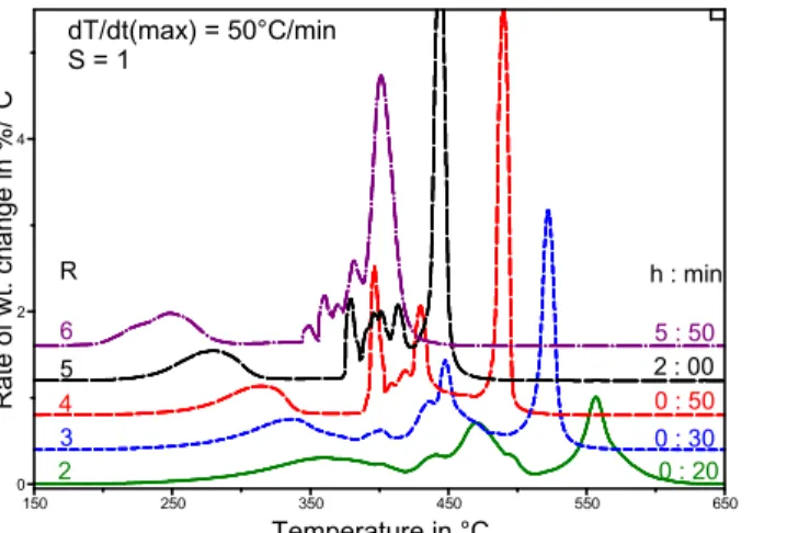
°C/min and 0.025 °C/min, respectively (Table 2). For any given heat rate, the minimum allowed rate may be expressed as a percentage of the maximum heat rate for any given R (Table 2). The effect of R, in the analysis of bitumen, for example, is well demonstrated in Fig. 3. As R increases, the response to a change in mass loss is faster and the allowed dT/dt(min) is reduced.
With any R value, the algorithm allows for the difference between dT/dt (max) and dT/dt(min) to be reduced with a sensitivity setting (S), which varies from 1 to 8. The default value of S=1 admits the full range of heat rates. Values of 2 and 3 reduce this range to about 50 % and 30 %, and higher S values reduce it further [19]. The effect of S is most easily understood by looking at the heat rate curves in Fig. 4. Below 350°C, a rising S provides for faster heating before a mass loss is detected and a faster drop in dT/dt once it is detected. After a mass loss, a rising S also leads to a more rapid increase in dT/dt, e.g. beyond 500 °C in Fig. 4. Consequently, a rise in S provides for conditions increasingly close to stepwise isothermal heating.
2.2.2 Constant decomposition rate. The other experimental approach provided
by the algorithms of Crowe and Sauerbrunn [17, 18] allows for maintaining a heat rate such that sample decomposition occurs at a constant rate. In this case, the dT/dt(max) is typically set at 5 °C/min in the absence of mass loss and possible R-values vary from – 0.1 to –8, and S-values vary from 1 to 8. When a mass loss is measured, the dT/dt varies so that dm/dt is constant until no more mass loss is detected. The value of this constant is set through R. Table 3 shows some values for R and the associated dm/dt in percent wt loss per min [19]: the lower the value of R, the lower the allowed sample decomposition rate and the longer the experimental time.
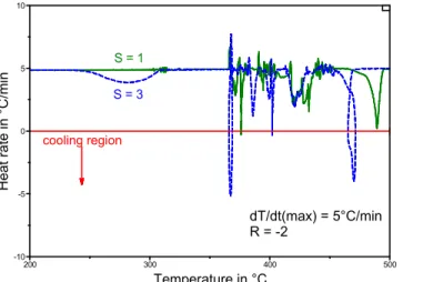
In the case of a reactive material where oxidation and decomposition may be rapid, S > 1 may help increase the resolution of the mass loss temperatures. An increase in S in the constant reaction rate experiment lowers the dm/dt threshold that will bring about a decrease in dT/dt, thus minimizing a possible overshoot of the decomposition temperature [TA manual 19]. Increases in S may thus lead to cooling, as most clearly illustrated for S=3 near 375°C and 475 °C in Fig. 5.
3. Experimental
3.1 Materials
Six bitumens and three polymer-modified bituminous sealants were used. One bitumen was an 85/100 penetration grade product from Petro-Canada. It served to develop the method. The other bitumens were obtained from the Materials Reference Library (MRL) of the Strategic Highway Research Program (SHRP) in the USA. They served to highlight the fingerprinting capability of the method. The bitumens were selected for their performance grade (PG) and for the difference in the origin of the crude oils from which they were obtained. Bitumens AAA, AAK and AAS were graded PG58-28, whereas bitumens AAG and AAM were respectively graded PG 58-10 and PG64-16 [1].
The bituminous sealants A, D, and E were amongst several used before [20, 21, 22]. They contained a styrene-butadiene type copolymer and a filler, most often calcium carbonate [20].
3.2 Methods
Masses of about 5 mg, unless otherwise indicated, were heated in a Q500 thermogravimetic analyzer from TA Instruments. The samples were heated in air, the flow being 60 mL/min. The heating conditions were controlled via the Advantage software for the Q Series, v2.0. For standard TGA, the linear heat rates varied from 1°C/min to 20 °C/min. In the varying heat rate experiments, the inputs were the resolution (R) and sensitivity (S) settings, and the maximum heat rate (dT/dt(max)). In the dynamic heat rate experiment, the maximum rate was 50°C/min. In the constant rate experiments, the maximum heat rate was 5°C/min. The results were analyzed with a Universal Analysis 2000 software, v3.9a from TA Instruments.
4. Results and discussion
4.1 Standard TGA
For the benefit of comparison, bitumen was first analyzed by means of standard TGA, in which the sample is heated at a constant rate. Fig. 6 shows results for rates of 1, 5, 10 and 20 °C/min. The DTGA profile generally shows three regions or peaks typical of heavy hydrocarbon mixtures [7=Herrington, 23]. At 20°C/min, for instance, a broad first peak of low intensity shows a maximum near 350°C; the most intense peak shows a maximum near 530°C; and between these limits is a series of poorly resolved and overlapping peaks. The first peak has been attributed to the distillation of low molecular weight material, and the others to thermal cracking and the loss of volatile fragments [24]. When it is resolved, the highest temperature peak has been used to quantify heavy bitumen fractions [4,9].
Fig. 6 shows that a reduction in the linear heat rate leads to a greater resolution of the low molecular weight material as it moves down in temperature, but it also leads to an increasingly poor resolution of the other peaks. Consequently, it is difficult to get a proper resolution of all the peaks with standard TGA.
4.1 Dynamic rates
The Petro-Canada bitumen was first analyzed in a series of experiments during which the effects of the R and S settings on the resolution of the various mass losses as
seen on the DTGA curve were compared. S and R were respectively varied from 1 to 5, and 2 to 6. The effect of some of these settings on the heat rate was shown earlier in Figs. 3 and 4. DTGA results for S=1 and R = 2 to 6 are shown in Fig. 7. For convenience, the first mass loss peak, which showed as a broad peak of low intensity, was labelled “light fraction”, the last mass loss peak was labelled “heavy fraction”, and the group of mass losses between the light and heavy fractions, was called the “middle fraction”, as initially illustrated in Fig. 2.
With R = 2 and 6, experimental times were respectively 20 min and ~6h (Fig. 7), in accordance with the effect of R on dT/dt (Table 2). With R=1 (not shown) or 2, the DTGA was much like standard TGA after heating at 20°C/min (Fig. 6). As R increased, the light fraction shifted to lower temperatures and resolved itself from the middle fraction starting at R = 4. In contrast, the heavy fraction was best resolved from the middle fraction with R ≤ 4. Hence, with S = 1, the separation of the light, middle and heavy fractions was best with R = 3 or 4.
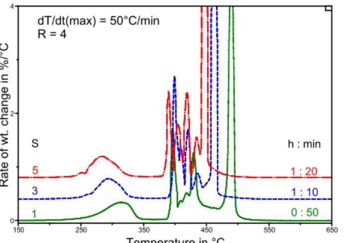
Building on the results with R=3 and 4, the effect of an increase in S was investigated. With R=3 and S=1, 3, and 5, the light fraction showed as a broad peak centered near 325°C, whereas the heavy fraction showed as a sharp and intense peak above 500°C (Fig. 8). The middle fraction showed multiple peaks between 375°C and 500°C that were best resolved at the higher sensitivity setting of S=5. In the experiments with R=4, an increase in S from 1 to 5 brought the light fraction to lower temperatures, but it decreased the resolution of the middle and heavy fractions as they came closer together (Fig. 9). The effect is much like that after a decrease in a linear rate of heating (Fig. 6). Consequently, the best conditions for bitumen analysis by means of the dynamic rate method were with R=3 and S=5 (Fig. 8). These settings gave the greatest resolution of the various fractions.
4.2 Constant reaction rate
The dynamic rate method only led to a broad and often unsymetrical peak for the light fraction. The shape suggested the overlap of at least two mass loss steps. In an effort to improve the sharpness of the signal from the light fraction, or deconvolute the underlying processes, the experimental conditions were changed to allow for a constant rate of volatile gas evolution. This required negative R-values and a low maximum heat rate, selected at 5°C/min. Fig. 10 shows the results for bitumen analyzed with S = 1 and R = –2 to –5. There was not much improvement in the profile of the light fraction with R at –2 and –3, but with R = –4 and –5, two partially resolved peaks were evident rather than a single broad one. Above 350°C, the DTGA profile was a succession of heating and cooling steps applied in an attempt to keep the rate of gas evolution constant at temperatures where bitumen is in its auto-ignition range [4]. The greatest control over the evolution of gases above 350°C was obtained when R was –2, conditions under which no cooling was applied.
Building again on these results, the effect of a varying S and a constant R of –2 on the resolution of the middle and heavy fractions was investigated. Fig. 11 shows the results when S was 1 and 3. With S = 3, the middle fraction, between 350°C and 450°C, showed 4 peaks with relatively good resolution of the various signals. Poor resolution was obtained with S=1.
4.3 Customized Methods
In reviewing the conditions investigated, it is obvious that one set of R and S values does not allow for the resolution of all bitumen fractions at all temperatures. The light fractions, with a mass loss peak below 350°C are best resolved under the conditions of a constant decomposition rate when R is –4 and S is 1 (Fig. 10). The middle fraction also shows a good resolution of its multiple peaks in this mode when R = –2 and S = 3 (Fig. 11), and in the dynamic rate mode when R is 3 and S is 5 (Fig. 8). In this latter mode, the heavy fractions were well resolved with an R of 3, regardless of the S value (Fig. 8).
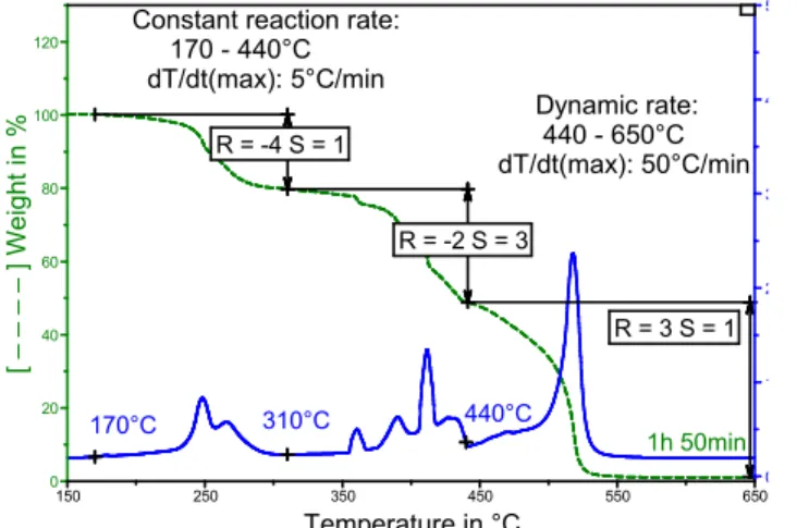
Given the above results, bitumen could be analyzed with a good resolution of its fractions under two sets of conditions (or two methods), both of which combine the constant reaction rate and dynamic rate conditions. With method-1 shown in Fig. 12, the conditions for a constant rate of reaction prevail from 170°C to 440°C, with a change in R and S at 310 °C. After 440 °C, the dynamic rate conditions are used. With method-2 shown in Fig. 13, the conditions for a constant rate of reaction only prevail up to 310°C, after which dynamic rate conditions are used.
The analysis of bitumen by means of these methods provides a fingerprint in less than 2h. The difference between bitumens of various sources will be shown later. With both methods, the light fraction shows as a doublet of peaks not completely resolved, with a less intense peak being on the high temperature side, and the heavy fraction shows as an intense peak near 500°C. The difference between the methods is mainly in the resolution of the middle fraction, which is heated under the conditions of a constant reaction with method 1, but heated under a dynamic rate in method 2. Given the extended temperature range where a constant reaction rate is found, method 1 might find an interesting application in the study of hydrocarbon degradation, especially as it relates to cracking and associated activation energies [25].
4.4 Reproducibility
To ascertain that reproducibility in the results is achieved, it is best that the sample in the TGA pan be of the same shape run after run. This is most easily achieved when the film is thin and flat. To get such a film, bitumen is pretreated so that it melts and flows to the bottom of the pan. For 5 mg of bitumen, 15 s at 170°C achieves the sought after results without a significant volatilization of material. Larger masses of about 12 mg and 22 mg led to a loss of resolution from the light fraction, as a single mass loss peak was obtained rather than two (Fig 14).
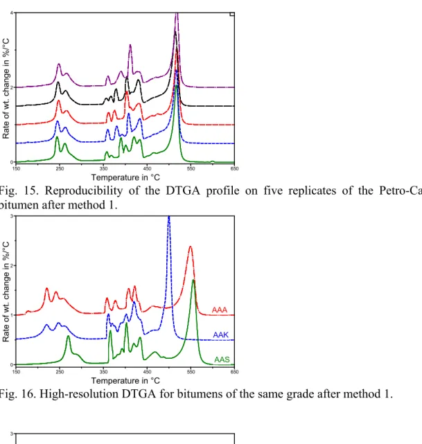
With a constant use of 5 mg of bitumen, the reproducibility in the profile of the light and heavy oils is excellent, with that between 350°C and 450°C showing a slight variation, most likely because of imperfect control of bitumen auto-ignition at these temperatures (Fig. 15). The peak temperature for the heaviest fraction varied within about 5°C, less than the difference between the peaks from different bitumens as will be seen shortly. The reproducibility in the mass loss at 325°C, 440°C and 700°C allows for the quantification of light, middle and heavy fractions in bitumen (Table 4). The standard deviation in the weight of the three fractions is better than 2%. Both the DTGA profile and the content of the various fractions may be used to fingerprint the material.
4.5 Applications
As stated in the introduction, it is often necessary to repeatedly use the same bitumen for the production of a bituminous product of consistent characteristics. In practice, this is often done by the purchase of a given bitumen grade from a single supplier. QC/QA upon reception of the raw material may be done with method-1 or -2 detailed above and the results compared with those from previous shipments. A positive identification is easily done given that bitumens of the same grade, but of different crude sources, show different DTGA profiles (Fig 16). As expected, bitumens of different grades also show different profiles (Fig. 17). Hence, a bank of TGA profiles may be built-up for the positive identification of any bitumen from a given process or source.
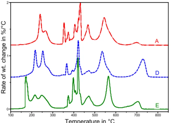
The methods can also be applied to the analysis of end products. The case of bituminous crack sealants is illustrated in Fig 18. Sealants contain a polymer, processing oils and a filler, in addition to bitumen [20]. The oils contribute to the light fraction and the polymer to the middle fraction. The filler shows as a weight loss beyond the heavy fraction, near 700°C. The results of detailed work on sealants will be provided in another publication.
5. Conclusion
Two high-resolution TGA/DTGA methods were developed by combining dynamic and constant reaction rate experiments. By applying the method, excellent resolution and reproducibility of about ten mass loss steps were achieved with bitumen and bituminous sealants. These results indicate that the TGA/DTGA method may be used for QC/QA applications and for the fingerprinting of such materials. The method shows potential for other applications, some examples being the quantification of bitumen fractions and that of components in end-products, and the study of cracking processes in heavy hydrocarbons.
Acknowledgements
The authors would like to thank Mr. Peter Collins for comments and suggestions during the preparation of the manuscript.
References
[1] D. R. Jones IV, SHRP Materials Reference Library for Asphalt Cements: A Concise Data Compilation. Report SHRP-A-645, Strategic Highway Research Program, National Research Council, Washington, D.C. 1993.
[2] J-F. Masson, P. Collins, G. Robertson, J. R.Woods, J. Margeson, Energy Fuels 17 (2003) 714.
[3] J-F. Masson, T. Price, P. Collins, Energy Fuels 15 (2001) 955.
[4] H. J. Völker, H. Fisher, Conf. Chem. Chem. Process Petrol. Natur. Gas, Budapest, 1965, p650-656 (in German).
[5] M. Wesołowski, Thermochim. Acta 46 (1981), 21.
[6] Anonymous, Hazardous Materials 6th edition, National Fire Protection Agency, 1975.
[7] P. R. Herrington, G. F. A. Ball, J. E. Patrick, Thermochim. Acta 202 (1992) 201. [8] S. M. Dyszel, Thermochim. Acta 38 (1980) 299.
[9] M. Václav, Hutn. Listy 23 (1968) 43 (in Slovak). [10] J. Rouquerol, Bull. Soc. Chim. (1964) 31.
[11] J. Rouquerol, Thermochim. Acta 144 (1989) 209. [12] J. Paulik, F. Paulik, Anal. Chim. Acta 56 (1971) 328. [13] F. Paulik, J. Paulik, Thermochim. Acta 100 (1986) 23. [14] O. T. Sorensen, Thermochim. Acta 13 (1978) 429.
[15] O. T. Sorensen, Proc. 5th Meeting of AICAT, AICAT, Trieste, 1983, p. 25. [16] W.J Sichina, American Laboratory 25 (1993) 45.
[17] B. S. Crowe and R. S. Sauerbruun, United States Patent 5,165,792, 1992. [18] B. S. Crowe and R. S. Sauerbruun, United States Patent 5,368,391, 1994.
[19] Anonymous, TA Instrument Operators Manual for Thermogravimetric Analyzer Q500, p. 30, 2001.
[20] J-F. Masson, P. Collins, J. Margeson, G. Polomark, Transportation Research Record 1795 (2002) 33.
[21] J-F. Masson, L. Pelletier, P. Collins, J. Appl. Polym. Sci. 79 (2001) 1034. [22] J-F. Masson, P. Collins, P-P. Légaré, Can. J. Civ. Eng. 26 (1999) 395. [23] B. Verkoczy, K. N. Jha, J. Can. Petrol. Technol. 25 (1986) 47.
[24] M. V. Kok, Thermochim. Acta 214 (1993), 315.
Table 1
Composition in percent wt of PG58-28 bitumens from different sources*
Bitumen AAA-1 AAK-2 AAS-2
Source Lloydminster Boscan Arab Heavy
Saturates 11 8 6 Naphtene Aromatics 32 31 46 Polar Aromatics 37 39 30 Asphaltenes (n-heptane) 16 19 17 * From [1]. Table 2
Effect of R on dT/dt(min) in dynamic rate experiments at specific dT/dt(max)
dT/dt(max),°C/mina R 50 20 10 5 1 % of dT/dt 1 10.02 4.01 2.00 1.00 0.20 20.03 2 3.68 1.47 0.74 0.37 0.07 7.37 3 1.36 0.54 0.27 0.14 0.03 2.71 4 0.50 0.20 0.10 0.05 0.01 1.00 5 0.18 0.07 0.04 0.02 0.01 0.37 6 0.07 0.03 0.01 0.01 0.01 0.13 7 0.02 0.01 0.01 0.01 0.01 0.05 8 0.01 0.01 0.01 0.01 0.01 0.02 a
experimental limit is 0.01 °C/min.
Table 3
Resolution settings and associated mass loss rates in the constant decomposition rate experiment. R dm/dt, %/min –1 10.000 –2 3.160 –3 1.000 –4 0.316 –5 0.100 –6 0.032 –7 0.010 –8 0.003
Table 4
Weight of the various fractions in the Petro-Canada bitumen as per method 1.
Replicate Light Middle Heavy
1 21.6 31.6 46.0 2 21.6 31.1 46.3 3 21.2 31.7 46.2 4 21.7 31.6 45.6 5 21.0 30.5 47.6 Av. Wt. (σ) 21.4 (0.3) 31.3 (0.5) 46.3 (0.8) % deviation 1.4 1.6 1.7
0.0 0.5 1.0 R a te of w t. c h a nge i n % /°C 150 250 350 450 550 650 Temperature in °C ––––––– run 1 – – – – run 2
Fig. 1. DTGA results from duplicate runs on bitumen heated at 20°C/min.
light fraction middle fraction heavy fraction 0 1 2 R a te of w t. c h a nge i n % /°C 150 250 350 450 550 650 Temperature in °C ––––––– High-resolution – – – – Standard
Fig. 2. Standard and high resolution DTGA for bitumen (dotted curve was shifted up for improved clarity).
dT/dt(max) = 50°C/min S = 1 3 R 14°C/min 4 6°C/min 0 10 20 30 40 50 Hea t rate i n °C/mi n 150 250 350 450 550 650 Temperature in °C 5 2°C/min 5 cooling region
Fig. 3. Effect of R on dT/dt in a dynamic rate experiment applied to bitumen. S 1 3 dT/dt(max) = 50°C/min R = 3 0 10 20 30 40 50 He at rate in °C/m in 150 250 350 450 550 650 Temperature in °C
Fig. 4. Effect of S on dT/dt in a dynamic rate experiment applied to bitumen.
dT/dt(max) = 5°C/min R = -2 S = 1 S = 3 -10 -5 0 5 10 Hea t rate i n °C/mi n 200 300 400 500 Temperature in °C
1 : 10 h : min 1 2 : 15 5 0 : 35 20 °C/min 0 1 2 Rate of wt. ch ang e in %/°C 150 250 350 450 550 650 Temperature in °C 1 : 10 10 4 0 : 50 5 0 : 30
Fig. 6. Standard DTGA on bitumen after heating at different rates. All the curves, except the bottom one, were shifted up for improved clarity.
dT/dt(max) = 50°C/min S = 1 2 0 3 0 : 30 5 2 : 00 R h : min 6 5 : 50 0 2 4 Rate of wt. ch ang e in %/°C 150 250 350 450 550 650 Temperature in °C : 20
Fig. 7. Effect of R on the bitumen DTGA profile after a dynamic rate experiment.
dT/dt(max) = 50°C/min R = 3 1 0 : 30 S h : min 3 0 : 30 0 2 4 Rate of wt. ch ang e in %/°C 150 250 350 450 550 650 Temperature in °C
1 0 : 50 S 3 1 : 10 dT/dt(max) = 50°C/min R = 4 h : min 0 2 4 Rate of wt. ch ang e in %/°C 150 250 350 450 550 650 Temperature in °C 5 1 : 20 -4 6 : 40
Fig. 9. Effect of S on the bitumen DTGA profile after a dynamic rate experiment.
dT/dt(max) = 5°C/min S = 1 -2 2 : 30 -3 3 : 20 -5 15 : 20 h : min R 0 2 4 Rate of wt. ch ang e in %/°C 150 250 350 450 550 650 Temperature in °C
Fig. 10. Effect of R on the bitumen DTGA profile after a constant reaction rate experiment. dT/dt(max) = 5°C/min R = -2 1 2 : 30 h : min S 3 2 : 10 0 2 4 Rate of wt. ch ang e in %/°C 150 250 350 450 550 650 Temperature in °C
Fig. 11. Effect of S on the bitumen DTGA profile after a constant reaction rate experiment.
1h 50min
170°C 310°C 440°C
Constant reaction rate: 170 - 440°C dT/dt(max): 5°C/min Dynamic rate: 440 - 650°C dT/dt(max): 50°C/min R = -4 S = 1 R = -2 S = 3 R = 3 S = 1 0 1 2 3 4 5 0 20 40 60 80 100 120 [ – – – – ] Weigh t in % 150 250 350 450 550 650 Temperature in °C
Fig. 12. Bitumen DTGA profile after the application of method 1, the R and S settings being as indicated. 1h 30min R = -4 S = 1 Dynamic rate: 310 - 650°C dT/dt(max): 50°C/min 170.00°C 310.00°C
Constant reaction rate: 170 - 310°C dT/dt(max): 5°C/min R = 3 S = 5 0 1 2 3 4 5 0 20 40 60 80 100 120 [ – – – – ] Weigh t in % 150 250 350 450 550 650 Temperature in°C
Fig. 13. Bitumen DTGA profile after the application of method 2, the R and S settings being as indicated. 12 mg 22 mg 0 1 Deri v. Weight (%/°C) 200 250 300 350 Temperature (°C) 5 mg
Fig. 14. Effect of the sample size on the DTGA profile of the light fraction of the Petro-Canada bitumen.
0 2 4 Rate of wt. ch ang e in %/°C 150 250 350 450 550 650 Temperature in °C
Fig. 15. Reproducibility of the DTGA profile on five replicates of the Petro-Canada bitumen after method 1.
AAK AAS 0 1 2 3 Rate of wt. ch ang e in %/°C 150 250 350 450 550 650 Temperature in °C AAA AAA
Fig. 16. High-resolution DTGA for bitumens of the same grade after method 1.
AAG AAM 0 1 2 3 Rate of wt. ch ang e in %/°C 150 250 350 450 550 650 Temperature in °C
D E 0 1 2 Rate of wt. chan ge i n % /° C 100 200 300 400 500 600 700 800 Temperature in °C A