Basic Spline Wavelet Transform
and Pitch Detection of a Speech Signal
by
Ken Wenchian Lee
Submitted to the Department of Electrical Engineering and Computer Science
in Partial Fulfillment of the Requirements for the Degrees of
Bachelor of Science
and
Master of Science
at theMassachusetts Institute of Technology
May 1994© 1994 Ken Wenchian Lee.
All rights reserved.
The author hereby grants to MIT permission to reproduce and to distribute
publicly paper and electronic copies of this thesis document in whole or in part.
//
of Author
by
. . .... . ... .. o d ;... .. . .. V1~ 4'.7 o.
Department of Electrical Engineering and Computer Science
... ... r...L.
Yr...
...
...-Professor Peter Elias
Department of Electrical Engineering and Computer Science
Thesis Supervisor (Academic)
by ...
;... ...
... ...
Dr. Forrest Tzeng
o-\
C
Supervisor
(COMSAT
Laboratories)
I .
by ...
·J... ...
deric R. Morgenthaleron Graduate Students
Signature
Certified
Certified
Accepted
Basic Spline Wavelet Transform and Pitch Detection of a Speech Signal
by
Ken Wenchian Lee
Submitted to the Department of Electrical Engineering and Computer Science
on January 28, 1994, in Partial Fulfillment of the Requirements for the Degrees of
Bachelor of Science
and
Master of Science
Abstract
In recent years the wavelet transform and its applications have gained tremendous interest
and have come under intense investigation. Successful applications of the transform are
inherently dependent on the wavelets themselves, whose properties necessary for a specific
application are not well known. In this thesis, besides examining wavelet theory, we study
the wavelet issues important in the accurate pitch detection of a speech signal in no noise,
low noise, and high noise environments.
To have control over the properties of the wavelets, we employ a transform based on
wavelets built from a sum of shifted B-spline functions. With these designed wavelets, the
transform is used to clarify the issues of support, smoothness, and viewing scale and their
importance. Performance in pitch detection is judged by how well the non-stationary
events of glottal closure are translated into local maxima in the transform coefficients and
how well these local maxima coincide with the actual instants of glottal closure.
Of all the experimental designs, the minimally supported, antisymmetric wavelet provides
the best performance in a no noise environment; in a low noise environment, the
performance is satisfactory; in a high noise environment, performance is satisfactory when
the wavelet shape is slightly altered. Performance of the wavelet in multi-speaker speech is also evaluated and is found to be very similar to that in noise.Thesis Supervisors:
Professor Peter Elias
Department of Electrical Engineering and Computer Science
Dr. Forrest Tzeng
Scientist, Voiceband Processing Department
COMSAT Laboratories
Acknowledgment
Very special thanks go to Dr. Tzeng, whose guidance and patience in not only this work but also previous assignments have made my VI-A experience at COMSAT
Laboratories enjoyable, memorable, and highly educational. I also would like to thank
Professor Elias at MIT and Dr. Unser at NIH for their guidance, comments, and advice.
Financial and technical support from COMSAT Laboratories, particularly the Voiceband Processing Department of the Communications Technology Division, is gratefullyacknowledged.
Table of Contents
A bstract ...
2
A cknow ledgm ent ...
3
Table of C ontents ...
4
List of Figures
...
List of Tables ...
14
Chapter 1
Introduction ...
15
Chapter 2
Fourier Analysis ...
17
2.1
Introduction ...
17
2.2
Fourier Series ...
17
2.3
Fourier Transform ...
18
2.4
Short-Time Fourier Analysis
...
20
2.4.1 Signal Analysis ...
20
2.4.2 Signal Expansion ...
25
2.4.3 Limitations of Short-Time Fourier Analysis ... 26
Chapter 3
Wavelet Analysis ...
28
3.1
Introduction ...
28
3.2
Historical Background ...
28
3.3
Wavelet Transform ...
30
3.3.1 Continuous Wavelet Transform ... 30
3.3.2 Discrete Wavelet Transform ...
34
3.3.3 Dyadic Wavelet Transform ...
36
3.3.4 Multiresolution Analysis, Dyadic Wavelet Basis, and Dyadic
Wavelet Transform ...
36
3.3.5 Dyadic Wavelet Transform via Filter Banks ... 40
3.3.6 Dyadic Wavelet Basis Construction ... 46
3.4
Wavelet Analysis vs. Fourier Analysis ... 49
3.5
Why the Dyadic Wavelet Transform? ... 51
Chapter 4
Basic Spline Wavelet Transform ... 54
4.1
Introduction ...
54
4.2
Historical Background ...
54
4.3
Basic Spline Functions and Polynomial Spline Interpolation ...56
4.4
Basic Spline Wavelet Transform ...
59
Chapter 5
Pitch Detection with the Basic Spline Wavelet Transform ...63
5.1
Introduction ...
63
5.2
The Pitch Detection Problem ...
63
5.3
Pitch Detection with Basic Spline Wavelet Transform ...74
5.4
Experimental Results and Discussion ... 76
5.4.1 Wavelet Shape ...
...
76
5.4.2 Approximating Spline Order and Viewing Scale ...88
5.4.3 Wavelet Support ...
94
5.4.4 Noisy Speech ...
102
5.4.5 Multi-speaker speech ...
108
5.4.6 Unvoiced Speech ...
113
Chapter 6
Conclusion ...
116
Appendix
A
...
.
... 18
A ppendix B ...
120
Appendix C ...
122
References
.. ...
125
List of Figures
Figure 2.4.1-1:
Figure 2.4.1-2:
Figure 2.4.1-3:
Figure 3.3.4-1:
Figure 3.3.4-2:
Figure 3.3.5-1:
Figure 3.3.5-2:
Figure 3.3.6-1:
Figure 3.3.6-2:
Figure 3.3.6-3:
Figure 3.3.6-4:
Figure 3.4-1: Figure 3.5-1:Figure 4.3-1:
Windowing operation of the STFT ...
20
STFT via filter banks ...
22
(a)
Implementing STFT with a bandpass filter ... 22
(b)
Implementing STFT with a lowpass filter ... 22
STFT basis functions; windowing and filter bank interpretations..24
(a)
STFT basis functions ... 24
(b)
Time-frequency plane illustrating both windowing and
filter bank views of the STFT ... 24
Decomposition of a signal into lower resolution components ...37
Reconstruction of higher resolution components of a signal ...38
Generation of lower resolution components with filter banks ...42
Generation of higher resolution components with filter banks ...43
Box function, scaling function for the Haar wavelet ...46
Haar wavelet ...
47
Daubechies scaling function ... 48
Daubechies wavelet function ... 48
Wavelet transform basis functions and time-frequency resolution
cells ...
50
(a)
Basis Functions ...
50
(b)
Time-frequency resolution cells ... 50
Octave-band filter banks of the dyadic wavelet transform ...52
B-spline construction ...
58
Figure 5.2-1: Figure 5.2-2: Figure 5.2-3: Figure 5.2-4: Figure 5.2-5:
(b)
First-order B-spline, 3 (t) ...
58
(c)
Second-order B-spline,
p 2(t) ...
58
Human speech production system ...
65
Opening and closing of the human vocal cords ... 66
Word and voiced speech frame ...
67
(a)
Time plot of the word "appetite" sampled at 8 kHz ...67
(b) 320 samples (40 ms) of the voiced sound \a\ at the front
of "appetite" ...
67
Clean and noisy test speech data ...
70
(a)
Clean ...
...
70
(b)
30 dB SNR ...
70
(c)
25 dB SNR ...
70
(d)
20 dB SNR ...
70
(e)
15 dB SNR ...
70
(f)
10 dB SNR ...
70
(g)
5 dB SNR ...
70
(h)
4 dB SNR ...
70
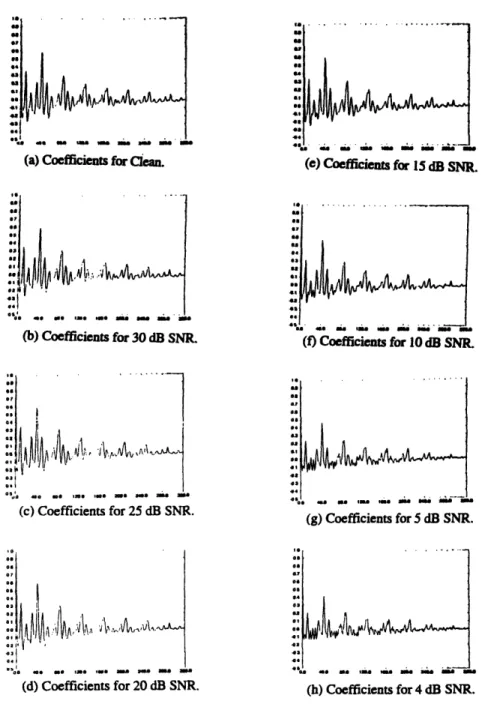
Normalized autocorrelation coefficients for clean and noisy test
speech samples.
For: ...
71
(a)
Clean ...
71
(b)
30 dB SNR ...
71
(c)
25 dB SNR ...
71
(d)
20 dB SNR ...
71
(e)
15 dB SNR ...
71
(f)
10 dB SNR ...
71
(g)
5 dB SNR ...
71
(h)
4 dB SNR ...
71
Figure 5.2-6: Figure 5.2-7: Figure 5.3-1: Figure 5.4.1-1: Figure 5.4.1-2: Figure 5.4.1-3: Figure 5.4.1-4: Figure 5.4.1-5:
Center clipping operation, C[] ...
72
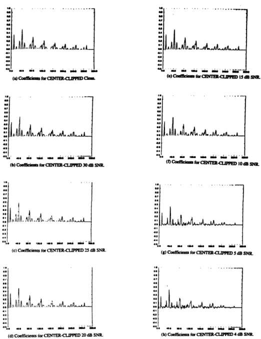
Normalized autocorrelation coefficients for CENTER-CLIPPED
clean and noisy test samples.
For: ...
73
(a)
Clean ...
73
(b)
30 dB SNR ...
73
(c)
25 dB SNR ...
73
(d)
20 dB SNR ...
73
(e) 15 dB SNR ... 73(f)
10 dB SNR ...
73
(g) 5 dB SNR ... 73(h)
4 dB SNR ...
73
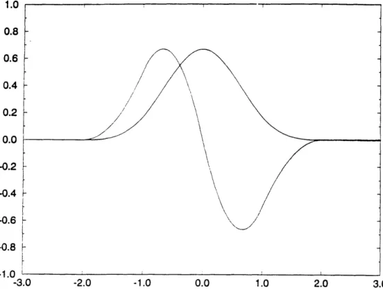
The smoothing cubic B-spline function and its first derivative, the
quadratic spline ...
75
W avelet W 1 ...
80
(a)
Shape ...
80
(b)
BSWT coefficients ... ...
80
Wavelet W2 ...
81
(a)
Shape ...
81
(b)
BSWT coefficients ...
81
W avelet W 3 ...
82
(a)
Shape ...
82
(b)
BSWT coefficients ...
82
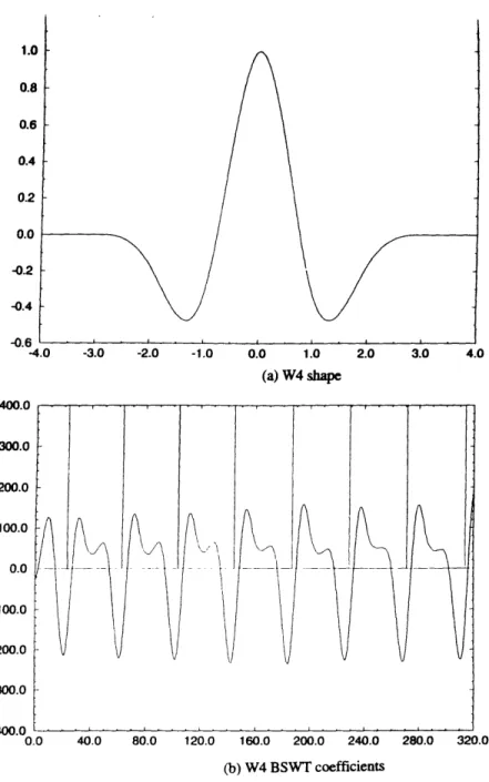
Wavelet W4 ...
83
(a)
Shape ...
83
(b)
BSWT coefficients ...
83
W avelet W 5 ...
84
(a)
Shape ...
84
Figure 5.4.1-6:
Figure 5.4.1-7: Figure 5.4.1-8:Figure. 5.4.2-1:
Figure. 5.4.2-2:
Figure. 5.4.2-3:
Figure. 5.4.2-4:
(b)
BSW T coefficients ...
84
Wavelet W6 ...
85
(a)
Shape ...
...
85
(b)
BSWT coefficients ...
85
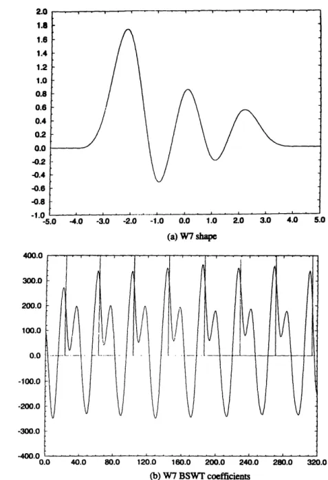
Wavelet W7 ...
86
(a)
Shape ...
... 86
(b)
BSWT coefficients .
...
86
Wavelet W8 ...
87
(a)
Shape ...
87
(b)
BSWT coefficients .
...
87
Wavelet W1 approximated with four different orders of
B-splines
...
89
BSWT coefficients based on WI approximated with st-order
B-splines and viewed at four different scales ... 90
(a)
m = 2 ...
90
(b)
m = 4 ...
90
(c)
m = 8 ...
90
(d)
m = 16 ...
90
BSWT coefficients based on WI approximated with 3rd-order
B-splines and viewed at four different scales ... 91
(a)
m = 2 ...
91
(b) m = 4 ... 91
(c) m = 8 ... 91
(d)
m = 16 ...
...
91
BSWT coefficients based on WI approximated with 5th-order
B-splines and viewed at four different scales ... 92
Figure. 5.4.2-5:
Figure. 5.4.3-1:
Figure. 5.4.3-2:
Figure. 5.4.3-3:
Figure. 5.4.3-4:
Figure. 5.4.3-5:
(b)
m = 4 ...
9
2
(c)
m = 8 ...
9
2
(d)
m = 16 ...
9
2
BSWT coefficients based on Wi approximated with 7th-order
B-splines and viewed at four different scales ... 93
(a)
m = 2 ...
93
(b)
m = 4 ...
93
(c)
m = 8 ...
93
(d)
m = 16 ...
93
Wavelet W 1 and its rescaled BSWT coefficients for clean
test data ...
96
(a)
Wavelet
W1 ...
96
(b)
Rescaled BSWT coefficients ...
96
Wavelet WA and its rescaled BSWT coefficients for clean
test data ...
97
(a)
Wavelet WA ...
97
(b)
BSWT coefficients ...
97
Wavelet WB and its rescaled BSWT coefficients for clean
test data ...
98
(a)
Wavelet WB ...
...
98
(b)
BSWT coefficients ...
98
Wavelet WC and its rescaled BSWT coefficients for clean
test data ...
99
(a)
Wavelet WC ...
99
(b)
BSWT coefficients ...
99
Wavelet WD and its rescaled BSWT coefficients for cleanFigure. 5.4.3-6:
Figure 5.4.4-1:
Figure 5.4.4-2:
Figure 5.4.4-3:
Figure 5.4.4-4:
(a)
Wavelet
WD ...
100
(b)
BSWT coefficients ...
100
Wavelet WE and its rescaled BSWT coefficients for clean
test data ...
101
(a)
Wavelet
WE ...
101
(b)
BSWT coefficients ...
101
Gaussian noise samples as test data and wavelet W1 BSWT
coefficients ...
104
(a)
320 samples of Gaussian noise ... 104
(b)
Wavelet W1 BSWT coefficients ... 104
Wavelet W 1 BSWT coefficients for eight different
test data SNR's ...
105
(a)
Clean ...
105
(b)
30 dB SNR ...
105
(c)
25 dB SNR ...
...
105
(d)
20 dB SNR ...
105
(e)
15 dB SNR ...
105
(f)
10 dB SNR ...
105
(g) 5 dB SNR ... 105(h)
4 dB SNR ...
105
Wavelet W a and its performance in high noise test data ...106
(a)
Wavelet W a q[k] parameters and shape ... 106
(b)
BSWT coefficients for 5 dB SNR test data ... 106
(c)
BSWT coefficients for 4 dB SNR test data ... 106
Wavelet W
3
and its performance in high noise test data ... 107
(a)
Wavelet WIP q[k] parameters and shape ... 107
Figure 5.4.5-1:
Figure 5.4.5-2:
Figure 5.4.5-3:
Figure 5.4.5-4:
(c)
BSW T coefficients for 4 dB SNR test data ... 107
Background speech ...
...
...
...
109
(a)
W ord ...
109
(b) Test data of 320 samples between the two vertical lines of
"destitute" ...
109
Dual-speaker speech test data at seven different SNR's ...110
(a)
30 dB SNR ...
110
(b)
25 dB SNR ...
110
(c)
20 dB SNR ...
110
(d)
15 dB SNR ...
110
(e)
10 dB SNR ...
110
(f)
5 dB SNR ...
...110
(g)
4 dB SNR ...
110
BSWT coefficients based on wavelet W1 for seven different
SNR dual-speaker test data ... 111
(a)
30 dB SNR ...
11
(b)
25 dB SNR ...
111
(c)
20 dB SNR ...
11
(d) 15 dB SNR ... 11 (e) 10 dB SNR ... 11(f)
5 dB SNR ...
11
(g) 4 dB SNR ... 111BSWT coefficients based on the wavelet W
Pfor dual-speaker
test data ...
112
(a) 10 dB SNR ... 112
(b)
5 dB SNR ...
112
Figure 5.4.6-1:
Figure 5.4.6-2:
Unvoiced speech test data .
... 114
(a)
Word ...
114
(b) 320 samples of unvoiced speech samples between the twovertical lines in (a) ...
114
BSWT coefficients based on wavelet W1 for 320 samples ofList of Tables
Table 5.4.1-1:
Table 5.4.3-1:
The q[k] coefficients of wavelets W1 -W8 ... 79
The q[k] coefficients of wavelets WA-WE
Chapter 1 Introduction
Recently, wavelet analysis and its applications have been under intense investigation in the scientific and engineering communities. A reason for this is that wavelet analysis elegantly unifies the seemingly disparate areas of wavelet series
expansions in applied mathematics, subband coding in speech and image processing, and multiresolution signal decomposition in computer vision [6]. In addition, the wavelet transform is potentially more useful in non-stationary signal analysis than traditional
Fourier methods.
A convenient way to view the wavelet transform is as a mathematical tool that decomposes a function onto a family of basis functions. But how well the transform fares in any application is inherently dependent on the choice of these functions. The objective of this work is a study of the factors and trade-offs involved in making these choices. The specific application under consideration is pitch detection of a speech signal, and the decision-making process learned from this application can be generalized for others.
Because our application deals with speech signals which are relatively smooth, we focus on wavelets built from smooth basic spline functions. But before we discuss the spline-based wavelet transform, some preliminary background information is presented. The thesis is organized as follows:
* Chapter 2 presents the methods and limitations of classical Fourier analysis, an important precursor of wavelet analysis. The presentation on the specific methods serves to preview the similarities and differences between the two analytical
frameworks. The limitations of Fourier analysis serve as a motivation to study and employ wavelet analysis.
· Chapter 3 deals with the wavelet transform: the continuous version, followed by the discrete and dyadic versions.
* Chapter 4 discusses the basic spline functions and the wavelet transform based on them.
* Chapter 5 furnishes the performances and evaluations of the basic spline wavelet transform in various pitch detection experiments.
* Chapter 6 concludes the experiments and the entire work.
Mathematical terminology used throughout the development of wavelet theory can be found in the Appendix A. Proofs are provided in Appendix B and C.
Chapter 2 Fourier Analysis
2.1 Introduction
In this chapter, the basics of classical Fourier analysis are presented so that their similarities and differences with wavelet analysis, which is discussed in the next chapter, will become more apparent. The first part (Sections 2.2 and 2.3) of the chapter is a brief review of the representation of periodic functions with the Fourier series and aperiodic functions with the Fourier transform. In the particular case of non-stationary signal analysis, short-time Fourier methods (Section 2.4) as an improvement over conventional Fourier methods are also included. The very last section of the chapter summarizes the limitations of the short-time Fourier transform in non-stationary signal analysis.
2.2 Fourier Series
The Fourier series is a convenient way to represent a finite-power periodic signal
f(t) in terms of a linear combination of complex exponentials,
f(t)
M
=
a
ne
- i"',
(2.2-1)
n=--o
where i =
1-7.
In other words, a T-periodic functionf(t) can be decomposed in terms ofmutually orthogonal basis functions, b(nt) = ein
', generated from integral dilations of the
prototypeb(t) = e',
(2.2-2)
I entmt
(b(nt), b(mt))
=ee'
dt
=,
for n m.
(2.2-3)
Here, (; ) denotes inner product.
Because the basis functions are mutually orthogonal, the series coefficients can be calculated as
To
In the signal processing literature, equations (2.2-1) and (2.2-4) are commonly referred to as the synthesis and analysis equations, respectively.
To further examine the series representation, let us substitute Euler's relation
e"' = cosnt
+
isinnt
(2.2-5)
into (2.2-1) yielding
f(t)= Zan cosnt + iZa
nsinnt,
(2.2-6)
n=--
n=--so that a periodic signal can aln=--so be represented as a sum of "sinun=--soidal waves" of distinct frequencies,
2r
In the case of aperiodic signals, an extension of the Fourier series effected by letting the period of the input signal approach infinity naturally leads to the Fourier transform.
2.3 Fourier Transform
Given a finite-energy aperiodic signalf(t), the Fourier transform (FT) analysis-synthesis pair are defined as
f(o) = f (t)e
idt
(analysis)
(2.3-1)
and
The transform maps a continuous-time signal onto the continuous-frequency domain. Signal energy is preserved according to the Parseval Relation,
Jlf(t)12 dt
=
]l
2do (2.3-3)However, in practice, the Fourier transform - also known as the natural "stationary transform"[6] - is rarely used. From the FT analysis equation, we see that the Fourier coefficient at frequency w tells us the prevalence of this frequency in the entire signal so that an integration over all time is required. When Euler's relation is substituted into (2.3-2), we see that an aperiodic signal is represented by sine waves localized in frequency but global in time. Such a representation is adequate only if the signal is made up of distinct stationary components. But such signals rarely exist. Furthermore, because any sudden change in time is reflected in the entire spectrum, the Fourier transform is inappropriate for signal analysis because it does not provide any information on the time location of
interesting spectral components.
The inadequacies of the FT can be summarized as
· Local changes in time are reflected in the entire frequency domain. · Lack of information on the time location of spectral components.
An extensively studied method devised to compensate somewhat for these inadequacies is the short-time Fourier transform, which is the topic of discussion of the next section. Chapter 3 discusses a better overall solution to these fundamental problems.
2.4 Short-Time Fourier Analysis
2.4.1
Signal Analysis
Instead of working with the entire signal, short-time Fourier analysis deals with a
windowed portion of it. For a window w(t), the short-time Fourier transform (STFT) of
f(t) is defined as
fsr(z,
o) = ff(t)w(t
-
r)e
-"
dt.
(analysis)
(2.4.1-1)
In the case of a discrete-time signalf(n) and a discrete-time window w(n), the STFT becomes
fsr(n, o) = Zf(m)w(n -m)e
-'",(analysis-discrete)
which says that the entire signal is windowed (Fig. 2.4.1-1) before the conventional
Fourier transform is taken.
Fgr W (n-rm)
m=n
Figure 2.4.1-1: Windowing operation of the STF1. (After Alien and Rabiner [2]).
While the FT furnishes an infinite-time spectrum of a signal, the STFT provides a short-time spectrum. And in contrast to the FT's need for signal stationarity, the STFT requires quasi-stationarity, i.e., the signal must be stationary within the time interval of interest. Hence, like a musical score, the STFT provides some information on the dependence of frequency on time [6].
The STFT analysis equation can also be viewed from a filter bank perspective. Rewriting the equation in terms of the Fourier transforms of the signal and window, f(o)
and iv(Wo), respectively, gives
jsTr(t,)
=
e
-Or
Jf()(w()e
idO
.
(2.4.1-3)
Thus, the coefficients can also be obtained by filtering f(t) with a bandpass filter and then demodulating the result back to the origin of the frequency axis (Fig. 2.4.1-2a). And if the order of the filtering and demodulation operations is reversed, a lowpass implementationresults (Fig. 2.4.1-2b).
f(t)
J ST L, W/J(a) Bandpass Filter
-iu
f(t)
(b) Lowpass Filter
Figure 2.4.1-2: STFT via filter banks. (a) Implementing STFT with a bandpass filter. (b) Implementing STFT with a lowpass filter.
Both the windowing and the filter bank interpretations of the STFT are illustrated in Fig. 2.4.1-3b. The horizontal axis corresponds to the time window interval, and the vertical axis to the filter bandwidth.
To examine the effectiveness of the STFT in signal analysis, we need to study its time-frequency resolution capabilities. Let a window and its Fourier transform be
represented as w(t) and w(o), respectively. The window's frequency bandwidth, Ao, is
defined asfST(',
CO)
A
fo 2¢(0) daco
A
co.-
=
(2.4.1-4)
Analogously, its time width At is
At =
(2.4.1-5)
For good time resolution, At should be as small as possible; for good frequency resolution, Aw should also be as small as possible. But since they must obey the uncertainty principle[8],
At AO 2
1,
(2.4.1-6)
2
a time-frequency resolution trade-off always exists. For maximum resolution, equality in
(2.4.1-6) must hold, which happens only when the window w(t) is Gaussian.
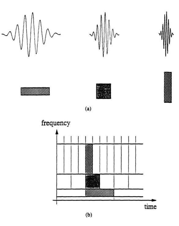
H
(a)
frequency
time
(b)
Figure 2.4.1-3: STFT basis functions; windowing and filter bank interpretations. (a) STFT basis functions.
(b) Time-frequency plane illustrating both windowing and filter bank views of the STFT. (After Vetterli and Herley [36]).
I. l i l II
E
. :i A I I2.4.2
Signal Expansion
The counterpart of the STFT analysis equation is the synthesis equation, or inverse short-time Fourier transform, which for a synthesis window g(t) is defined as ([4], [7])
f(t)
=
2r
I
.J.
ST('
r(o)[g(t-
)ei]drdo,
(synthesis)
(2.4.2-1)
where , o E 9?. Unlike the FT's basis functions which are infinite-duration complex exponentials, those of the STFT have finite duration (Fig. 2.4.1-3a).
Hlawatsch and Boudreaux-Bartels have interpreted the window g(t) as centered at
( r = 0, o = 0) in the time-frequency plane (Fig. 2.4.1-3b) [7]. The coefficient fsT(Z, w)
then corresponds to the contribution of the time-frequency point ( r = 0, o =
O0)to the
decomposition off(t). Each rectangle in the time-frequency plane (Fig. 2.4.1-3b) corresponds to a resolution cell for signal representation. For exact reconstruction, the analysis and synthesis windows must satisfy [4]fg(t)w(t)dt
=
1.
(2.4.2-2)
So far we have considered an expansion of a signal in terms of a continuous time-frequency plane, but a discrete time-time-frequency plane can also be used. The discretized
versions of the STFT analysis and synthesis equations, (2.4.1-1) and (2.4.2-1),
respectively, are ([4], [7])f (aT, bw) = f f(t)w(t -ar)e
-ib dt
(discrete-analysis) (2.4.2-3)
and
f(t)= .
fST(aT,bco)[g(t - a)eb
"]. (discrete-synthesis)
(2.4.2-4)
a=--
b=--where a, b E Z. The condition required to ensure exact reconstruction becomes [7]
-2
g(t
+-
-aT)w(t -aT)
=
3[b],
t 9'.
(2.4.2-5)
An interesting point to make here is that the signal expansion of equation (2.4.2-4) can be generalized as
f (t)
=
I
LCa,b
ha,b(t),(2.4.2-6)
a=-ob=-,
where hu,b(t)
=h(t
-aT)e
i bx,a, b E Z. Equation (2.4.2-6) is commonly known as the
Gabor expansion of a continuous-time signal into shifts of the window h(t) and scaled versions of the Fourier kernel e. Maximum time and frequency localization occurs only when h(t) is Gaussian. And if the window in the STFT is Gaussian, the resulting
transform is also known as the Gabor transform.
2.4.3
Limitations of Short-Time Fourier Analysis
Though short-time Fourier methods are an improvement over conventional Fourier methods for non-stationary signal analysis, they are still very inadequate. The efficacy of the STFT depends on the assumption that an input signal is stationary within the window of interest so that any non-stationarities within this window will only affect the short-time spectrum. Unlike the Fourier transform, in which any sudden change in time is reflected throughout the spectrum, the STFT has, in essence, localized the spectral disturbances. Hence, the effectiveness of this approach depends critically on the window's time width.
According to the definition of the STFT (equation (2.4.1-1)), only shifts of the window are used for analysis so that two pulses less than a window time width apart cannot be distinguished. Such inflexibility renders the STFT inappropriate for many signal analysis problems, e.g., pitch detection of a speech signal in which pitch pulses vary from
1.25 ms to 40 ms apart [85].
The limitations of the STFT can also be studied from a signal expansion perspective: that is, to study a signal, we decompose it with respect to a set of basis functions and hope the interesting parts of the signal will be more evident in this
decomposed form. In contrast to the infinite-duration basis functions of the Fourier transform, those of the STFT are finite. However, this duration is constant (Fig. 2.4.1-3a). Unless we know how fast the signal is changing, the STFT is highly inflexible - and perhaps even inappropriate. If we assume the signal is extremely fast-changing, and therefore, choose a window with an extremely small time width so that we do not lose any detail, the amount of computation involved will render the method impractical.
In summary, the constancy in both window width and basis function duration of the STFT makes it an unattractive tool for non-stationary signal analysis. The wavelet transform, discussed in the next chapter, is a generalization of the Gabor expansion, and by relaxing the constancy restrictions of the STFT, it is more attractive - and potentially more useful - in non-stationary signal analysis, although it still must obey the uncertainty principle.
Chapter 3 Wavelet Analysis
3.1 Introduction
While the basics of the Fourier methods are covered in Chapter 2, this chapter deals with the theoretical and interpretational aspects of the wavelet methods. Section 3.2 provides a brief historical background. Section 3.3 discusses various kinds of wavelet transforms: continuous, discrete, and dyadic. Also included are their properties and interpretations from multiresolution and filter bank perspectives. Section 3.4 delineates the differences in signal analysis capabilities between the Fourier and wavelet methods. The last section discusses some of the reasons for the great interest in the wavelet transform as a signal processing tool, especially in the areas of image and speech processing.
Note that some of the mathematical terminology used throughout this chapter are defined in Appendix A. Proofs are provided in Appendix B and C.
3.2 Historical Background
Although explicit wavelet analysis did not come into play until a decade or so ago, something very similar has existed since 1946 when Gabor proposed a method to study a signal more carefully by shifting an analyzing function along the time and frequency axes. The most popular function used in such a capacity is the Gaussian, in which case the Gabor transform results. As far as signal analysis is concerned, the Gabor transform is better than
the STFT because maximum time-frequency localization prevails. However, the Gabor transform still has the same fundamental limitations as the STFT.
About a decade ago a fundamentally better transform was introduced by Grossman and Morlet [26]. Their method deals with the decomposition of functions into "elementary wavelets," which arise from dilations and translations of a single basic wavelet. Early applications in seismic analysis have found it to be numerically stable. Unlike the Gabor transform which may cause numerical instability when a very high frequency transient signal is reconstructed from the Gaussian basis functions, the newly introduced transform does not possess this liability. The mathematical foundations presented in [26] has spurred theoretical studies and novel applications.
Daubechies et al. [25] investigates the transform from an applied mathematical point of view: that is , the expansion of a function in terms of a chosen set of basis functions. If the set constitutes an orthonormal basis, the functional expansion in terms of a linear combination of these functions converges. But to achieve orthonormality, the functions
themselves sacrifice smoothness (i.e., number of continuouse derivatives), or regularity.
If the function to be expanded happens to be smooth, the basis will most likely produce extraneous transform coefficients and may introduce false high-frequency components. Non-orthogonal, or quasi-orthogonal, basis functions have also been studied and they have been found to be very useful in some areas of signal analysis, in particular edge detection[35], zero-crossing determination [62], ventricular delayed potentials in the electrocardiogram [32], and seizure detection in the electroencephalogram [57].
Though very important, the issues and trade-offs among the properties of orthogonality, functional support, regularity, and complexity in the basis functions have
not been very well studied. For a specific application, a carefully considered compromise among the properties needs to be made. The following chapters of this thesis attempt to elucidate what such a compromise entails.
3.3 Wavelet Transform
3.3.1
Continuous Wavelet Transform
While the basis functions of the Fourier series and Fourier transform are infinite in duration and those of the STFT are windowed versions of the same kind of functions, we would like to do better. We would like the functions themselves to be "small waves," or
wavelets [12], which decay rapidly to zero, and thereby obviate any use of windows. In
addition, these functions must span L2( 9) space. And like the complex exponentials, they must have frequencies. In summary, the functions should possess:
* Fast decay.
* A span of the L (9r) space.
· Frequency.
To construct such a basis, we first need a starting function which we can
manipulate to create a family of functions. To obtain fast decay, one has to select a starting function that has this property. For the basis to span the entire L2(99) space, one can shift the original function so that the support of the basis covers the entire real axis. To obtain all frequencies, we can contract and dilate the original. For example, for a functionf(t) with a domain of [0, 1], the contracted version, f(2t), has twice as many variations within the same domain, while the dilated version,f(t/2), has half as many.
Let the original wavelet be
(t)
EL2(9), also called the mother wavelet. The
constructed basis becomes
fa.b(t)
=V(
-),
a,
b
E9.
(3.3.1-1)
Parameter b shifts, or translates, the motion wavelet along the time axis; parameter a scales the rapidity, which is the same kind of scale used in road maps and serves as an analogue of frequency w in Fourier analysis. For a function f(t) e L2(9') and a basis
!a,b(t) E L2(9i), the continuous wavelet transform (CWT) is defined as
(CWT7,
f)(b, a)
=
a
f(t) tl
) dt,
(3.3.1-2)
a
where a -Y2 is a normalization factor, and the overhead bar denotes complex conjugation.
In terms of an inner product, the definition can be expressed as
(CWT7,
f)(b,a)
= lal-2(f(t), ya,b(t)).
(3.3.1-3)
The CWT can also be expressed in terms of Fourier transforms:
(CWT
0f)(b,a)
=J(w)
eiboiO(aw) do,
(3.3.1-4)
where i = -'.
Not every function in L2(9i) can be a wavelet. The necessary conditions are:
V(t) E L(9
')(3.3.1-5)
and
j fli(O)I
dw
< 00*(3.3.1-6)
Iol
The latter condition is commonly known as the admissibility condition, and a function that obeys this condition is said to be admissible. Let us see where this condition originates.
Since the basis is built from a mother wavelet, it must be the case that the constructed family of functions can be projected back onto this "mother" function.
Working in Hardy space (see Appendix A), H2(9?), Grossman and Morlet [26] formulate
this requirement mathematically as
(e/2
Yr(et
- v),
l(t))
du dv
< o,
(3.3.1-7)
where u, v 9t, and
a
= eu and b -= are substituted into the CWT definition. Thederivation of the admissibility condition from equation (3.3.1-7) can be found in Appendix
B. In practical terms, for a function ty(t)to qualify as a wavelet,¢(ro=0) = o,
i.e., the function must have an average of zero:
f V(t)dt = 0.
(3.3.1-8)
Now to see how the CWT can be used to process signals, we look into some of its properties:
* Linearity: CWT is linear. N
Proof: Let f(t) =Z fn(t), where n, N
E
n=I(CWT, f )(b, a)
- lal 2 __ n=/Z, N> 1, and fn(t)
L
2(9i), then
f, n(t
)
t-b ) dt.
a
Interchanging the two linear operations, namely integration and
(CWT, f at
-)dt
(CWT,
f)(b,a) = Za
-
f
(- )dt.
'(t)
n=l _
a
summation, gives
According to the CWT definition, N
(CWT, f)(b,a) = Z(CWT, fn)(b,a).
n=l
* Shift in time: CWT is time-shift invariant.
Proof: Let
fT(t) =f(t
-
T)
EL2(W9),
where f(t)
EL(9t)
and T
E
9?, then
(CWT fT)(b, a)
=
la
-
2f (t
-
T) (t
-b
)dt.
a
Let v = t -T. Substitutingdt = dv
andt-b=v-(b-T)
into (CWT, fT)(b, a) yields(CWTv
fT)(b, a)
(CWT, fT)(b, a)
= lalY2
Jf(v)(v-(b-
T))dv,
a
= (CWT f)(b -T,a).
* Scale change: CWT is scale-change invariant.
Proof: Let fc(t)
=
Icl2
f (ct) E L
2(9), where f (t)
E
L2(9?),
c E 9, and c > 0, then(CWT, fc)(b, a)
= a Y2 c2f(ct)
(-)dt. Let v = ct. Substitutingdt =
dv
C andt-b
v -cb
a cainto the above equation, we obtain
(CWTv
fc)(b,a)
= al/2lcICl
2f(v)
v-cb)
dv
ca c
= (CWT, f )(cb, ca).
Energy preservation: The CWT preserves signal energy. Specifically, and V(t) is admissible, then
-
fl(CWT, f)(b, a)l
2dadb
=f
(t) dt,
Cu/
....
a'
-'if f(t)
L
2(97)
(3.3.1-9)
where
c, = |
)do.
(3.3.1-10)
A proof can be found in Appendix C.
* Inverse transform: For f(t) E L2 (9?) and (CWT, f )(b, a) E L2(9i), the inverse CWT
is defined as
I
-y t-b
1
f(t)
=-
j
ai
2
l(
)(CWT, f)(b, a) dadb, (3.3.1-11)
cy/
a-a
where c, is defined in (3.3.1-10). A proof can be found in [26].
Just by examining the definition, we see that the CWT can be a very flexible and useful signal analysis tool. There is much freedom in choosing, or designing, them for a specific application. An early application of the CWT was in transient signal analysis, in which Tuteur [32] used different dilation parameters, I/a, to pinpoint abnormalities in an electrocardiogram. The distinct parameters chosen were; /a = 11, 16, and 22. Hence, although the CWT is very useful, in most cases, the transform is not taken over all dilation
parameters because, in practice, a small number of parameters suffices. When the CWT is taken over all continuous parametric values, it is highly redundant; besides, such an undertaking is extremely computationally burdensome. In short, to be of practical use, the transform must be simplified.
A natural way to simplify the CWT is to discretize the dilation and translation parameters, a and b, which leads to the discrete wavelet transform (DWT).
3.3.2
Discrete Wavelet Transform
To discretize the parameters a and b in the CWT definition, let us choose a = Mi
and b = kM;N, where M, N E 9? and j, k E Z. Expressing the CWT in terms ofj and k
results in the definition of the discrete wavelet transform (DWT):(DWT, f)(k, j) = M
Jf(t)
f
(M-it -kN)dt.
(3.3.2-1)
An analogous formulation in terms of Fourier transforms is
(DWT, f)(k, j)
=
M/;
jf(o)
ir(MiJ)eilM'N° do.
(3.3.2-2)
Here, the wavelet basis functions are M V(M-it - kN). While the CWT maps a signal
onto a continuous a-b plane, the DWT projects it onto a discrete j-k grid.
Some of the properties of the DWT are very similar to those of the CWT, and so their proofs are omitted in the following list:
* Linearity: The DWT is linear.
* Energy preservation: The DWT preserves energy.
* Inverse transform: An original signal f(t) E L2(9W) can be reconstructed from its DWT
coefficients as
f(t) =
I
(DWT,f)(k,j)M
r(Mt-kN).
(3.3.2-3)
* Shift in time: The DWT is time-shift variant.
Proof. Let
fT(t) =f(t
-T), where
f(t)
EL
2(9i)
and T
E9?, then
(DWT, fT)(k,j) =
MA
Jf(t-T)yV(M-t-kN)dt.
(3.3.2-4)
Let v = t - T. Substituting
dt = dv
andt=v+T
into (3.3.2-4) yields(DWT,. fT)(k, j)
= M
ff(v) (M-ijv
-(k
)N)dv. (3.3.2-5)
M-_
Since in general, T • T, then
N
(DWT,
fr)(k,j) # (DWT,f)(k-T,j).
(3.3.2-6)
* Scale change: DWT is scale-change variant.
Prooff Let f(t)
=
Icly f(ct) E L
2(9W), where f(t) E L
2(9), c 9?, and c > 0, then
(DWT, fc)(k,j)
= MA
JfcIY2f(ct)
y(M
-t-kN)dt.
(3.3.2-7)
Let v = ct. Rewriting (3.3.2-7) in terms of v gives
MAwr~f,,ia~i
f-v)
I,(lfrWM'
dv
(DWT,
fc)(k,j)
= m
c|2
f(v)v(M
-i -kN)-. (3.3.2-8)
Further simplification leads to
(DWTt fc)(k, j)
•(DWT, f)(ck, cj).
(3.3.2-9)
The lack of time-shift invariance of the DWT means that for the transform to be
meaningful, the time location must be specified.3.3.3
Dyadic Wavelet Transform
1 Interesting interpretations and simple implementation arise when we choose M -
-2
and N = I in the definition of the discrete wavelet transform, in which case the dyadic wavelet transform results:
(WT, f)(k,j)
=
2J
f
ff(t)
y(2
't -k)dt,
(3.3.3-1)
where j, k E Z. Here, all scales, (2j), and all shifts, (2- i ), are dyadic. Unlike the DWT, the dyadic wavelet transform has properties which are very similar to those of the CWT. In
particular, it is time-shift invariant and scale-change invariant (Proofs of these properties are very similar to those of the CWT). But unlike the CWT, it is much less redundant.
The basis functions of the WT2, are 2i
rI(2'
t - k). An interpretation of thesefunctions from a multiresolution signal decomposition point of view and their relationship with filter banks are the topics of discussion of the following sections.
3.3.4
Multiresolution Analysis, Dyadic Wavelet Basis, and
Dyadic Wavelet Transform
A very interesting interpretation of the dyadic wavelet basis can be obtained from multiresolution analysis. To fully appreciate this point of view, let us review a signal processing technique that is often viewed as an important precursor of multiresolution
analysis.
The theory of multiresolution analysis, currently very popular in computer vision and image processing, is built upon the Laplacian pyramid algorithm introduced by Burt
and Adelson [60] in 1983. Since images tend to have high pixel-to-pixel correlation, the main goal of the pyramidal scheme is to remove as much correlation as possible to effect a net data compression. To simplify our review, let us assume that the original signal, So, is one-dimensional. The algorithm starts off by low-pass filtering So. If L[.] denotes the low-pass filtering operation and Lo denotes the low-pass filtered, or blurred, version of the signal, then
Lo = L[So],
and the residual component, R, can be represented as
R = So - Lo.
Now if we again apply the filtering operation to the already low-pass filtered signal Lo, we have
L, = L[Lo],
and another residual signal results,
R = Lo - L.
The alternating filtering and subtraction operations can be continued until the signal is decomposed satisfactorily, in which case we end up with the residual components,
Ro, RI, ..., R, and a most blurred remnant of the original signal, L,. Fig. (3.3.4-1)
summarizes the decomposition stage of the pyramidal algorithm. To reconstruct a signal, a complementary technique is used; Fig. (3.3.4-2) illustrates the reconstruction stage of the pyramidal algorithm.
So -- Lo, I
*--
-- L,Ro R R Rn
S
o+-
1o
'
+-
L.
-
L"
Ro R, R
Figure 3.3.4-2: Reconstruction of higher resolution components of a signal.
Because the residual components, Rn's, and the most blurred component, L, are decorrelated, only they will be encoded.
The idea of representing a signal at different resolutions (e.g., an original image as an order hierarchy of blurred images) serves as the foundation of Mallat's multiresolution approximation framework ([24], [27], [33]), which involves approximating a function,
f(t) E L2(9?), at different resolutions and is described in the rest of this section.
Let us form a basis made up of shifts of a certain function s(t) along the time axis
Sk(t)
= s(t-k),
k EZ,
such that the basis spans a subspace of L2(9?), V. In other words,
V
O= span[Sk(t)}.
Employed in such a capacity, s(t) is commonly known as the scaling function. Let us now generate a family of functions by scaling the set of shifted spanning functions, or
sj,(t) = 2
4
s(2Jt-k), j,k
Z.
(3.3.4-1)
For a given j, a certain subspace Vj is spanned by sj, k(t). As j increases the size of the spanned subspace also increases, and an ordered hierarchy of bigger and bigger subspaces can be built:
... cV
c
V
o
V
c...
c V
(3.3.4-2)
such that
Vj c Vj+. (3.3.4-3)
In addition, as j -- o, the entire
L
2(9) space is spanned; analogously, as j - - oo thenull space is spanned:
V_- = {o0.
The nesting of subspaces (implied in (3.3.4-3)) means that for any function f(t) e L2(9i),
f(t) E Vj
f(2t) E Vj,.
(3.3.4-4)
Now that we have seen that bigger and bigger subspaces can be spanned by scaling functions, let us investigate how the residual information between two consecutive
subspaces can be represented. Since this residual information is very similar to that briefly discussed in the Laplacian pyramidal algorithm, it can be represented in a similar way.
Hence, let Wj denote a subspace that is the orthogonal complement of Vj, or
Wj V = = V V. (3.3.4-5)
A projection of a signal onto Wj yields a representation of the residual information. Analogous to the generation of the basis that spans Vj, a basis built from dilations and translations of a wavelet, (t), can be used to span Wj. The resulting basis is
YIj.k(t)
= 2"2 (2jt- k),
j,
kZ,
(3.3.4-6)
which is same as that used in the definition of the dyadic wavelet transform (equation(3.3.3-1)).
From the nesting of the V subspaces and the orthogonal complementarity between the subspaces Wj and Vj, an important result arises. By repeatedly substituting Wj subspaces of lower resolution for the V+,, subspaces, we see that the entire L2(9?) space can be spanned by a sum of Wj subspaces, or
...
0
Wj
Wj,
Wj
,
I
...
= L
2.
(3.3.4-7)
Consequently, when an arbitrary function needs to be analyzed, the wavelet functions will
suffice.
3.3.5 Dyadic Wavelet Transform via Filter Banks
From the previous section, we see that the dyadic wavelet transform can be used as a way to carry out multiresolution analysis. But such a multiresolution decomposition, or mathematically, a projection onto the different subspaces, needs to be carried out
efficiently. A fast method based on filter banks does exactly this.
From the nesting of subspaces (equations (3.3.4-2) and (3.3.4-4)), a fundamental
relationship between the scaling functions of two consecutive scales exists:s(t) =
g(k)s(2t-k),
(3.3.5-1)
k=-o
which is known as a two-scale difference equation. From (3.3.4-5), we deduce that
Wi c V+, ,or
I(t) =
Zh(k)s(2t-k).
(3.3.5-2)
k=--Burrus and Gopinath [22] have shown how a filter bank interpretation of the dyadic
wavelet transform results from a manipulation of equations (3.3.5-1) and (3.3.5-2).
(Hereafter, for the purpose of clarity, the taking of the dyadic wavelet transform implies multiresolution decomposition and vice versa.)Now let us see how a signal decomposition can be carried out with filter banks. Since Wj 6 Vj = Vj,;, if f(t) E Vj+ then
f(t) =
a
j+,
2s(2i+'t - k),
(3.3.5-3)
k=--or
f(t) =
Zaj(k)2'
s(
2it-k) +
Zb(k)2)2/
y(2t-k).
(3.3.5-4)
k=--- k=-
s(2it-k)
= Zg(n-2k)s(2j+'t-n)
(3.3.5-5)
n=--and
1(2't-k)
=
h(n-2k)s(2j+'t-n).
(3.3.5-6)
To solve for the coefficients a(k) in (3.3.5-4), we need to multiply both sides of
(3.3.5-4) by 22
s(2i
t -
k)
and integrate with respect to t. If the bases s,
kand yj
,kare
orthonormal, then because they are also orthogonal complements of each other, we obtain
fj(t)2/
s(2it -k)dt = aj(k).
(3.3.5-7)
If s(2i t - k) is replaced with (3.3.5-5), the coefficients can be generated recursively as
aj(k) =
g(n - 2k)aj+,(n).
(3.3.5-8)
The coefficients b (k) can be solved for in a similar manner. After multiplying
(3.3.5-4) by
22(2 t - k) and integrating with respect to t, we have
jf(t)2
y(2Jt-k)dt
=
bj(k).
(3.3.5-9)
Further manipulation leads tobj(k) = Zh(n - 2k)aj,(n).
(3.3.5-10)
From the above derivation, we see that equations (3.3.5-8) and (3.3.5-10) provide us with a fast way to decompose a signal into a series of lower resolution components. In
fact, for a signal represented at resolution j+l, the lower resolution components can be
obtained by filtering and downsampling by a factor of two. This process can be repeated toobtain lower and lower resolution components (Fig. 3.3.5-1).
bj-,
Figure 3.3.5-1: Generation of lower resolution components with filter banks.
An equally attractive way to reconstruct a signal from its lower resolution
components also exists. Setting equation (3.3.5-3) equal to (3.3.5-4) yields
a aj+,(k)2
+
s(2
;
" t-
'
k) =
.a(k)2
s(2t- k) +
(3.3.5-11)
bj;(k)22
yf(2Jt-k).
k=--If we substitute equations (3.3.5-1) and (3.3.5-2) into the right side of (3.3.5-1 1), multiply
both sides of (3.3.5-1 1) by s(2
j+'t - k) before integrating with respect to t, we have
ajI,(k) =
a(n)g(k-2n) + b(n)h(k-2n).
(3.3.5-12)
n.--
n=--Hence, a signal represented at resolution j+l can be obtained by first upsampling by a
factor of two the coefficients at resolution j and then filtering with the same filters that are
used during the decomposition stage. The procedure can be repeated to rebuild the signal at
higher and higher resolutions (Fig. 3.3.5-2).
bj-,
Figure 3.3.5-2 : Generation of higher resolution components with filter banks.
This fast multiresolution decomposition-reconstruction algorithm is attributed to Mallat, and
a more detailed derivation can be found in [22], [24], and [36].To further study how the filter implications of equations (3.3.5-1) and (3.3.5-2) are
related to subband coding techniques, let us first take the Fourier transform of both sides of
(3.3.5-1) such that
s(co
=
g(e )5( 2),
(3.3.5-13)
2 2 where(ei
)-=
Zg(k)e
-"
~.
k=--If the family of functions, s(t - k), k
EZ, is orthogonal with respect to each other, then
according to the Poisson formula [18], equation (3.3.5-13) implies that the following holds
in the frequency domain:14S(co + 2k) 2 = 1, (3.3.5-14)
k=-which also means that
JS(2co
+ 2kr)l
= 1.
(3.3.5-15)
=-_
Let us now examine the implications of equations (3.3.5-14) and (3.3.5-15). First,
replace in (3.3.5-13) with 2 so thatS(2w)
=I(e")S((w).
(3.3.5-16)
2
Next, replace co in (3.3.5-16) with + kir to obtain
s(2wo
+
2kr)
I=
(e+i(+k))s(+ kr).
(3.3.5-17)
2After taking the absolute value, squaring, and summing over all k on both sides of (3.3.5-17), we have
1.(2o)
+
2kir)
2
=
g(e(+k
)2
S( + kTr)
+-
2.(3.3.5-18)
k=-oo 4k=--,
Substituting (3.3.5-15) into the left side of (3.3.5-18) yields
4 =
ZI
(ei('"+k')l
2[i(to
+ kr)12.
(3.3.5-19)
k=--Since (e'w) is a 2nr-periodic function, we can rewrite (3.3.5-19) in terms of even and
odd k's, so that
4 = (e
) '+
22klr)
+
(3.3.5-20)
ZV(ei+(2k+°)| 2
Is(w +
(2k
+ 1)2.
k=--When (3.3.5-14) and (3.3.5-15) are substituted into (3.3.5-20), we have
4 = + I(ei("+')+(e"Ol2 l, 2
(3.3.5-21)
which is the defining equation for a class of perfect reconstruction quadrature mirror filters (QMF), which have been extensively studied and applied in subband coding [30]. Since QMF's deal with one low-pass and one band-pass filter, we need to identify these filters.
Multiplication of both sides of (3.3.5-1) by dt followed by an integration with
respect to t gives2 =
Ig(k),(3.3.5-22)
k=--or
which says that (e' ) is actually the low-pass filter. A similar analysis shows that h(ei' ) is the band-pass filter. From the QMF relationship, the filter sequences, g(k) and h(k), are related by
h(k)
=
(-)k
g(-k
+
1).
(3.3.5-24)
So far we have seen that decomposing and reconstructing a signal involve simple filtering operations. An interesting filtering interpretation of the scaling and wavelet functions also exists. From the orthogonality of the scaling equation with its translates along the time axis, Mallat in [27] has shown that the scaling function is actually a low-pass filter. Likewise, due to the orthogonality of the mother wavelet with its translates, he has found that the wavelet function also represents a band-pass filter. Thus, because sjk (t)
spans Vj and 1
j.k (t) spans Wj, whenever we talk about mapping a function onto the V
and Wj subspaces, this simply corresponds to low-pass and band-pass filtering it,
respectively, in signal processing terminology.
3.3.6 Dyadic Wavelet Basis Construction
One of the simplest ways to construct a dyadic wavelet basis is to start with the coefficients, g(k), of the two-scale difference equation, (3.3.5-1). Having the coefficients, one needs to find a scaling function that satisfies (3.3.5-1). The overall heuristic approach is very similar to solving a differential equation.
Burrus and Gopinath [22] have developed a much more structured method. By using the fact that the scaling function and its integer translates are orthogonal. they imposed another constraint on the coefficients. They first select the number of non-zero values in g(k). From the number of coefficients supported by g(k) and the orthogonality
constraint, they solve a system of equations based on equation (3.3.5-1) for g(k).
Once g(k) and s(t) are determined, h(k) and the wavelet function, t t), can be
obtained by equations (3.3.5-24) and (3.3.5-2), respectively. To see if V(t) is a mother
wavelet, one needs to check whether f
(t) dt = 0 holds.
Let us now look at some popular wavelets. The simplest one is the Haar wavelet. The Haar scaling function is
SHaar(t) = o:henrwae (3.3.6-1)
which is also known as a box function (Fig. 3.3.6-1).
1.20 -1.00 0.80 0.60 0.40 0.20 -0.00- -.1.00 .0.50 0.00 0.50 1.00
![Figure 3.3.6-3: Daubechies scaling function. (After Daubechies [23])](https://thumb-eu.123doks.com/thumbv2/123doknet/14144728.470991/48.918.244.639.100.364/figure-daubechies-scaling-function-after-daubechies.webp)
![Figure 3.5-1: Octave-band filter banks of the dyadic wavelet transform. (After Rioul and Vetterli [6]).](https://thumb-eu.123doks.com/thumbv2/123doknet/14144728.470991/52.918.166.701.808.985/figure-octave-filter-dyadic-wavelet-transform-rioul-vetterli.webp)
![Figure 5.2-1: Human speech production system. (After Flanagan [88])](https://thumb-eu.123doks.com/thumbv2/123doknet/14144728.470991/65.918.280.635.237.824/figure-human-speech-production-flanagan.webp)