An automated reliable method for two-dimensional Reynolds-Averaged Navier-Stokes simulations

An Automated Reliable Method for

Two-Dimensional Reynolds-Averaged Navier-Stokes

Simulations

by

James M. Modisette

S.M., Massachusetts Institute of Technology (2008)

B.S., Massachusetts Institute of Technology (2005)

Submitted to the Department of Aeronautics and Astronautics

in partial fulfillment of the requirements for the degree of

Doctor of Philosophy

at the

MASSACHUSETTS INSTITUTE OF TECHNOLOGY

fS P9

ARCHIVES

September 2011

©

Massachusetts Institute of Technology 2011. All rights reserved.

Author... ... . . . . . . . .

Department of'Aeronautics and Astronautics

N

C ertified by ...

David A. armofal

Professor of Aeronautics and Astronautics

Thesis Supervisor

C ertified by ...

Robert Haimes

Principle Research Engineer

r

.Thesis Committee

Certified by ...

S

C/

Qiqi Wang

Assistant Professor of Aeronautics and Astronautics

If

Thesis Committee

Accepted by ...

Eytan H. Modiano

Professor of eronautics and Astronautics

Chair, Committee on Graduate Students

An Automated Reliable Method for

Two-Dimensional Reynolds-Averaged Navier-Stokes Simulations

by

James M. Modisette

Submitted to the Department of Aeronautics and Astronautics on August 18, 2011, in partial fulfillment of the

requirements for the degree of Doctor of Philosophy

Abstract

The development of computational fluid dynamics algorithms and increased computational resources have led to the ability to perform complex aerodynamic simulations. Obstacles remain which prevent autonomous and reliable simulations at accuracy levels required for engineering. To consider the solution strategy autonomous and reliable, high quality solu-tions must be provided without user interaction or detailed previous knowledge about the flow to facilitate either adaptation or solver robustness. One such solution strategy is pre-sented for two-dimensional Reynolds-averaged Navier-Stokes (RANS) flows and is based on: a higher-order discontinuous Galerkin finite element method which enables higher accuracy with fewer degrees of freedom than lower-order methods; an output-based error estimation and adaptation scheme which provides quantifiable measure of solution accuracy and au-tonomously drives toward an improved discretization; a non-linear solver technique based on pseudo-time continuation and line-search update limiting which improves the robust-ness for solutions to the RANS equations; and a simplex cut-cell mesh generation which autonomously provides higher-order meshes of complex geometries.

The simplex cut-cell mesh generation method presented here extends methods previously developed to improve robustness with the goal of RANS simulations. In particular, analysis is performed to expose the impact of small volume ratios between arbitrarily cut elements on linear system conditioning and solution quality. Merging of the small cut element into its larger neighbor is identified as a solution to alleviate the consequences of small volume ratios. For arbitrarily cut elements randomness in the algorithm for generating integration rules is identified as a limiting factor for accuracy and recognition of canonical element shapes are introduced to remove the randomness. The cut-cell method is linked with line-search based update limiting for improved non-linear solver robustness and Riemannian metric based anisotropic adaptation to efficiently resolve anisotropic features with arbitrary orientations in RANS flows. A fixed-fraction marking strategy is employed to redistribute element areas and steps toward meshes which equidistribute elemental errors at a fixed degree of freedom. The benefit of the higher spatial accuracy and the solution efficiency (defined as accuracy per degree of freedom) is exhibited for a wide range of RANS applications including subsonic through supersonic flows. The higher-order discretizations provide more accurate solutions than second-order methods at the same degree of freedom. Furthermore, the cut-cell meshes demonstrate comparable solution efficiency to boundary-conforming meshes while signifi-cantly decreasing the burden of mesh generation for a CFD user.

Thesis Supervisor: David L. Darmofal

Acknowledgments

I would like to express my gratitude to the many people who have made this thesis possible. First, I would like to thank my advisor, Professor David Darmofal, for giving me the oppor-tunity to work with him. I am grateful for his guidance, inspiration and encouragement.

In addition, I would like to thank my committee members, Bob Haimes and Professor Qiqi Wang, for their criticism and feedback, which led to many improvements in my research and this thesis. I am appreciative of my readers Professor Krzysztof Fidkowski and Dr. Mori Mani for providing comments and suggestions on this thesis. I am also grateful to Dr. Steve Allmaras for the time he devoted to the ProjectX team and his help with the non-linear solver modifications.

Of course, this work would not have been possible without the efforts of the entire ProjectX team past and present (Julie Andren, Garrett Barter, Laslo Diosady, Krzysztof Fidkowski, Bob Haimes, Josh Krakos, Eric Liu, Todd Oliver, Mike Park, Huafei Sun, David Walfisch, Masa Yano). There is no way this work would ever have been completed without their help. Special thanks goes to Laslo who has been my companion and office mate for our entire time in the ACDL, putting up with my habits and questions and being a good friend to me. I am indebted to Masa who has become a close friend always willing to listen whether I have a research topic to discuss, something to complain about, or a joke to tell.

I would like to thank my parents, Jim and Ruth, for their constant support, without which I am sure I would not have gotten this far. My extended family, Kerry and Bob, deserve recognition for the encouragements and positive distractions they provided me. I must also thank Mora, whose has been the pillar of support for my graduate studies. Her love and friendship propelled my progress and enabled this work.

I have sincerely enjoyed the many friendships I developed through both my undergraduate and graduate years at MIT. In particular, Chuck, Boshco, Dan, Jack, Jake, Kalin, Fran, Kozbi, and Moscow have all helped to make MIT more fun than it might otherwise have been.

Finally, I would like to acknowledge the financial support I have received throughout my graduate studies. This work was partially supported by funding from The Boeing Company with technical monitor Dr. Mori Mani. The guidance I received from weekly teleconferences with Boeing employees helped keep my work grounded to practical CFD applications.

Contents

1 Introduction 17

1.1 M otivation . . . . 17

1.2 O bjectives . . . . 19

1.3 Solution Strategy Background . . . . 20

1.3.1 Higher-Order Method . . . . 20

1.3.2 Output-Based Error Estimation and Adaptation . . . . 21

1.3.3 Cut-Cell Mesh Generation . . . . 24

1.4 Thesis Overview . . . . 27

2 Discretization of the RANS-SA Equations 31 2.1 The RANS Equations . . . . 31

2.2 The SA Turbulence Model . . . . 32

2.3 Spatial Discretization . . . . 35

2.4 Shock capturing . . . . 39

3 Non-Linear Solution Technique 43 3.1 Pseudo-Time Continuation . . . . 43

3.2 Pseudo-Time Solution Update . . . . 46

3.3 Line-Search Solution Update Limiting . . . . 47

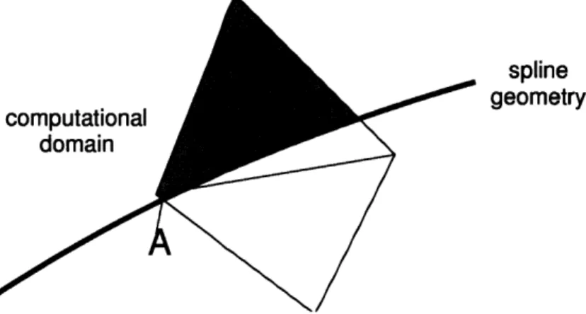
4 Cut-Cell Mesh Generation 51 4.1 Geometry Definition . . . . 51

4.2 Intersection Algorithm . . . . 53

4.3 Integration for Arbitrary Element Shape . . . . 58

4.4 Canonical Shape Recognition . . . . 63

4.5 Solution Basis Space . . . . 67

5 Small Volume Ratios 75 5.1 Boundary Derivative Outputs with Small Volume Ratios . . . . 81

5.2 Analysis of the Conditioning of a One Dimensional Problem with Small Vol-um e R atios . . . . 85

5.2.1 D efinitions . . . . 85

5.2.2 Bilinear form to linear operator . . . . 86

5.2.3 Restriction to finite element space . . . . 87

5.2.4 Condition number for operators between Hilbert spaces . . . . 88

5.3 5.4

5.2.6 Relate stiffness matrix to Hilbert space setting . . . . 5.2.7 Matrix condition number - quasi-uniform mesh . . . . 5.2.8 Matrix condition number - mesh with a small volume ratio 5.2.9 Implications of ,c(A) = !0(h- 2)0(VR-1) . . . . Modified Discretization Space c'...

Model Problem Results . . . .

6 Output-Based Error Estimation and Adaptation

6.1 Output-Based Error Estimation . . . . 6.2 Adaptation Strategy . . . . 6.2.1 Fixed-Fraction Marking . . . . 6.2.2 Anisotropy Detection . . . . 6.2.3 Limit Requested Element Metrics . . . . 6.2.4 Generation of Continuous Metric Field . . . . 6.2.5 6.2.6 6.2.7 . . . . 90 . . . . 92 . . . . 96

. .. . ..

103

. .. . ..

104

. .. . ..

116

. .. . ..

118

Metric Request Construction and Explicit Degree of Freedom Control Building Metric Request for Null Cut Elements . . . . DOF- "Optimal" Mesh . . . . 7 Results 7.1 Comparison of Boundary-Conforming and Cut-Cell Solution Efficiency 121 122 124 129 . . . 129

7.1.1 NACA0012 Subsonic Euler . . . . 7.1.2 RAE2822 Subsonic RANS-SA . . . . 7.1.3 RAE2822 Transonic RANS-SA . . . . 7.1.4 NACA0012 Supersonic RANS-SA . . . . 7.1.5 Multi-element Supercritical 8 Transonic RANS-SA . 7.1.6 Summary . . . . 7.2 Surface Quantity Distributions . . . . 7.3 DOF-Controlled Adaptation for Parameter Sweeps . . . . . 7.3.1 Fixed Mesh vs. Adaptive Mesh . . . . 7.3.2 Comparison of Boundary-Conforming and Cut-Cell . 7.4 Comparison of Boundary-Conforming and Cut-Cell Solution . . . 129 . . . 132 . . . 134 . . . 137 . . . 143 . . . 145 . . . 146 . . . 152 . . . 152 . . . 157 "Cost" . . . 157 8 Conclusions 8.1 Summary and Contributions. . . .. . .. . . . . .. . . . . 8.2 Future W ork . . . .. . . . . Bibliography 165 . . . 165 . . .. ... 167 170

List of Figures

1-1 Computed drag convergence for a wing-alone configuration at Moo = 0.76, a =

0.5*, and Re = 5 x 106 with global mesh refinement taken from Mavriplis [85]. Convergence of drag is plotted for the refinement of two mesh families of the same wing geometry. . . . . 18 1-2 Convergence history for p = 0 -+ 3 of RANS simulations of an RAE2822

airfoil (M,,, = 0.734, a = 2.79*, Rec = 6.5 x 106, 8,096 q = 3 quadrilateral elements) taken from Bassi et al.[18]. . . . . 19 1-3 Illustration of the autonomous output-based error estimation and adaptation

strategy. . . . . 22 1-4 Diagram of the options for converting a linear boundary conforming mesh to

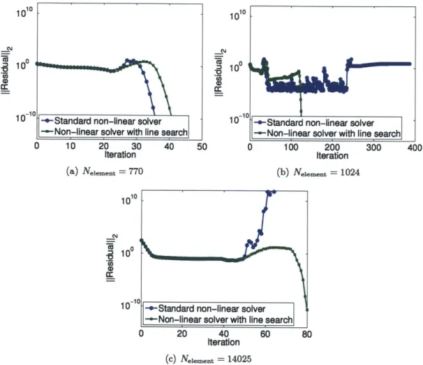
a mesh containing higher-order geometry information. . . . . 25 3-1 Residual convergence for three boundary-conforming meshes for a subsonic

simulation of the RANS-SA equations over the RAE2822 airfoil (M = 0.3, a = 2.31, Re = 6.5 x 106). . . . . 50 4-1 Example of spline geometry representation of a NACA0012 airfoil. The spline

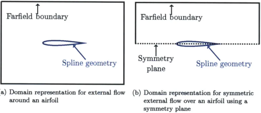
parameter, s, defines the computational domain to be external to the airfoil. . 52 4-2 Illustration of embedded and farfield domain representation for external flow

over an airfoil. . . . . 52 4-3 Illustration distinguishing different zerod, oned, and twod objects within a

cut grid. . . . . 53 4-4 Degenerate intersection cases. . . . . 54 4-5 Illustration of oned objects at the leading edge of an airfoil. . . . . 55 4-6 Illustration of typical cut elements at an airfoil trailing edge. The left

back-ground element straddling the airfoil is treated as two cut elements with each cut element defined by separate loops of oned objects. The arbitrarily cut element at the trailing edge is a single cut element with four neighbors. The direction of the Loop is shown for the element at the trailing edge. . . . . 57 4-7 Example of a cut-cell mesh for a NACA0012 airfoil. The spline geometry is

shown in red. . . . . 58 4-8 An example of the "speckled" 2D integration points for a cut-cell mesh. In

order to support p = 5 solutions, upwards of 484 points are suggested to adequately cover the interior of the element. . . . . 59 4-9 An example domain used with the two-dimensional scalar convection-diffusion

4-10 Example of a boundary-curved domain. The boundary-conforming domain is globally linear with a single curved boundary on the geometry surface. . . . . 60 4-11 Plot of the heat flux distribution along the inner radial boundary of the

com-putational dom ain. . . . . 61 4-12 Convergence history of the minimum and maximum heat flux distribution

error at solution orders 1 though 5, where 100 different sets of "speckled" points are used for integration rules at the four grid refinement levels. . . . . 62 4-13 Range of heat flux distribution error over a 100 sets of "speckled" points at

p = 5 for each grid refinement level. . . . . 62 4-14 Triangles and quadrilaterals are recognizable canonical element shapes and

improve the quality of the integration rules. The example elements are the canonical version of the cut elements shown in Figure 4-8 with their canonical

quadrature points. . . . . 63 4-15 Conversion of a three-sided cut element to a higher-order canonical triangle.

A q = 5 Lagrange basis is used for the illustration. . . . . 64 4-16 Maps for element and solution representation. . . . . 68 4-17 Two mesh families used to examine the effect of a Cartesian basis compared

to a parametric basis on solution accuracy . . . . 70 4-18 Comparison of the convergence in the heat flux distribution errors for cases

with parametric and Cartesian approximation functions on globally curved higher-order meshes and globally linear meshes with a single curved boundary. The plots indicate, although there is a small deterioration in the error and rates with the Cartesian functions, the Cartesian functions still perform well at higher order, even in boundary-curved meshes. . . . . 71 4-19 Illustration of linear shadow element options from typical cut elements at an

airfoil's trailing edge. The * indicates the preferred option given the element

type... ... 72

5-1 Example of a small volume ratio. Usually, small volume ratios occur when a grid node is just inside the computational domain. . . . . 75 5-2 Diagram of mesh when grid has uniform h except for the first element where

h= hVR... ... 77

5-3 Plot of solution and its derivative for the one-dimensional model problem. The exact solution is plotted along with computed solutions for Nelement = 16, p = 3 and VR = 1 and VR = 10-8. The inset figures show the solution at

the left boundary . . . . ... *. 78 5-4 Derivative of the solution for the one-dimensional model problem plotted in

the reference space of the leftmost element in the domain with a VR = 10-8,

Nelement = 16, p = 3. . . . . 78 5-5 The convergence of the L2 solution error with varying critical volume ratio.

Due to the tiny size of the element with the critical volume ratio, the small volume ratio has no impact on the L2 error. . . . . 79 5-6 The convergence of the broken H' solution error with varying critical volume

ratio. The critical volume ratio has no impact on the H1 error. . . . . 79 5-7 The convergence of the error in the output J(u) = v, 1 for a range of

5-8 Plot showing the variation of the condition number versus element size and

volume ratio for the one-dimensional model problem. . . . . 81

5-9 The convergence of the error in the output J(u) = vg for a range of volume ratios for the one-dimensional model problem, Equation (5.1). The selection of

p

e)

(f, )

#

5-10 Diagram relating the equivalence of the actions of the the interpretation op-erator, Ih, and the Hilbert space opop-erator, Ah, to the action of the matrix, A, and the functional interpretation operator, I4, on Euclidean space, R". (Taken from [73]) . . . . . .. . ... 92

5-11 The effect of nudging node 1 to eliminate the small volume ratio associated

with elem ent A. . . . 105

5-12 Illustration of the effect of merging element A into element B. The resulting element, C, maintains the solution basis of element B and the quadrature points are taken from both element A and B. . . . 106

5-13 Original and merged domains for the one-dimensional model problem. ei and e2 are merged to form em. . . . 106

5-14 The convergence of the error in the output

gd

I

#1)-(f,

#1)

5-15 Convergence of the heat flux distribution error for cut-cell meshes on the two-dimensional model problem. The errors in boundary-conforming cut cases are compared to the errors in cut meshes with small volume ratios that have either been merged out or remain. . . . 107

5-16 Boundary distributions of heat flux for the two-dimensional convection-diffusion problem using merged and non-merged cut grids. . . . 109

6-1 Mesh metric-field duality. . . . 115

6-2 Flow chart detailing a single adaptation step. . . . 116

6-3 Fixed fraction adaptation strategy . . . 117

6-4 An example of a limited metric which corresponds to the maximum element coarsening. . . . 121

6-5 Multiply-cut element where the requested metric for element A is passed to nodes 1 and 2 but not node 3... 122

6-6 Cut elements intersecting a viscous wall form a wake-like feature in the back-ground m esh. . . . 124 6-7 Example describing the process of forming requested metrics on null elements. 124 6-8 Example of the initial and DOF-"optimal" meshes for subsonic RAE2822

RANS-SA flow (Mo, = 0.3, Rec = 6.5 x 106, a = 2.31*, p = 3, DOF = 40k). . 125 6-9 The the error estimate, the error, the drag, and the degree of freedom

adap-tation history for a set of initial meshes applied to the subsonic RAE2822 RANS-SA flow (Moo = 0.3, Rec = 6.5 x 106, a = 2.31*, p = 3, DOF = 40, 000).126

7-1 Mach number distribution, initial mesh, and the DOF-"optimal" meshes for

subsonic NACA0012 Euler flow (Moo. = 0.5, a = 2.00). The Mach contour lines are in 0.05 increments. . . . 130 7-2 Envelopes of drag coefficients and cd error estimates for subsonic NACA0012

Euler flow (Moo = 0.5, a = 2.0*). . . . 131

7-3 Mach number distribution, initial mesh, and the DOF-"optimal" meshes for for subsonic RAE2822 RANS-SA flow (Moo = 0.3, Rec = 6.5 x 106, a = 2.31'). The Mach contour lines are in 0.05 increments. . . . 132 7-4 Envelopes of drag coefficients and cd error estimates for subsonic RAE2822

RANS-SA flow (Moo = 0.3, Rec = 6.5 x 106, a = 2.31*). _{. . . 133} 7-5 Mach number distribution, initial mesh, and the DOF-"optimal" meshes for

subsonic RAE2822 RANS-SA flow (Mo = 0.729, Rec = 6.5 x 106, a = 2.31*). The Mach contour lines are in 0.025 increments. . . . 134 7-6 Envelopes of drag coefficients and cd error estimates for transonic RAE2822

RANS-SA flow (Moo = 0.729, Rec = 6.5 x 106, a = 2.31'). . . . 136

7-7 The Mach number distribution for the supersonic NACA0006 RANS-SA flow (Moo =2.0, Rec = _{106, a = 2.00) and the DOF-"optimal" meshes obtained}

for p = 1 and p 3 at 80k degrees of freedom adapting to drag. The Mach contour lines are in 0.1 increments. . . . 138 7-8 Envelopes of drag coefficients and ca error estimates for supersonic NACA0006

RANS-SA flow (Moo = 2.0, Re_ = 106, a = 20). . . . 139

7-9 Envelopes of pressure signal and error estimates for supersonic NACA0006 RANS-SA flow (Moo = 2.0, Rec = 106 a = 2.0*). . . . 141

7-10 The pressure perturbation distribution, (p(u) - poo) /poo, for the supersonic NACA0006 RANS-SA flow (Moo = 2.0, Rec = 106, a = 2.5*) and the DOF-"optimal" meshes obtained for p = 1 and p = _{3 at 80k degrees of freedom}

adapting to the pressure signal 50 chords below the airfoil. . . . 142 7-11 Mach number distribution, initial mesh, and the DOF-"optimal" meshes for

transonic MSC8 RANS-SA flow (Moo = 0.775, Rec = 2.0 x 107, a = -0.7*). . 143 7-12 Envelopes of drag coefficients and Cd error estimates for transonic MSC8

RANS-SA flow (Moo = 0.775, Rec = 2.0 x 107, a = -0.7*). . . . 144 7-13 Coefficient of pressure surface distributions for cut-cell and boundary-conforming

meshes at DOF = 40k and DOF = 160k for subsonic RAE2822 RANS-SA flow (Mo = 0.3, Rec = 6.5 x 106, a = 2.31*). The drag error estimates associated with each distribution are in drag counts. . . . 147 7-14 Coefficient of skin friction distributions for cut-cell and boundary-conforming

meshes at DOF = 40k and DOF = 160k for subsonic RAE2822 RANS-SA

flow (Mo, = 0.3, Rec = 6.5 x 106, a = 2.310). The drag error estimates

associated with each distribution are in drag counts. . . . 149 7-15 Coefficient of pressure surface distributions for cut-cell and boundary-conforming

meshes at DOF = 40k and DOF = 160k for transonic RAE2822 RANS-SA flow (Moo = 0.729, Rec = 6.5 x 106, a = 2.310). The drag error estimates associated with each distribution are in drag counts. . . . 150

7-16 Coefficient of skin friction distributions for cut-cell and boundary-conforming meshes at DOF = 40k and DOF = 160k for transonic RAE2822 RANS-SA

flow (Moo = 0.729, Rec = 6.5 x 106, a = 2.310). The drag error estimates associated with each distribution are in drag counts. . . . 151 7-17 Comparison of skin friction distribution for boundary-conforming meshes and

cut-cell meshes using a critical volume ratio of VRcrit = 10-5 and VRcrit = 10-1 at p = 1, 2,3 and DOF = 160k. Transonic RAE2822 RANS-SA flow (Moo = 0.729, Rec = 6.5 x 106, a = 2.310). . . . 153 7-18 The lift curve and the c1 error obtained using the fixed mesh and adaptive

meshes for the three-element MDA airfoil. . . . 154 7-19 The error indicator distribution, logio(r7s), for the three-element MDA airfoil

at a = 23.28* obtained on the 8.10* optimized mesh and the 23.28* optimized

mesh. ... ... 155

7-20 The Mach number distribution for the three-element MDA airfoil at a = 23.280 obtained on the 8.100 optimized mesh and the 23.280 optimized mesh. The Mach contour lines are in 0.05 increments. . . . 155 7-21 The initial and lift-adapted grids for the three-element MDA airfoil at selected

angles of attack. . . . 156 7-22 Envelopes of drag coefficients and cd error estimates for a = 8.10 MDA

RANS-SA flow (Moo = 0.2, Rec = 9 x 106). . . . 158 7-23 Envelopes of drag coefficients and Cd error estimates for a = 16.21* MDA

RANS-SA flow (Moo =0.2, Rec = 9 x 106). . . . 159

7-24 Envelopes of drag coefficients and Cd error estimates for a = 21.34* MDA

RANS-SA flow (Moo = 0.2, Rec = 9 x 106). . . . 160 7-25 Envelopes of drag coefficients and Cd error estimates for a = 23.28* MDA

RANS-SA flow (Moo = 0.2, Rec = 9 x 106). . . . 161 7-26 cl error estimate convergence with adaptation iteration during generation of

lift curve for MDA RANS-SA flow (Moo = 0.2, Rec = 9 x 106) with boundary-conforming and cut-cell meshes. . . . 162

List of Tables

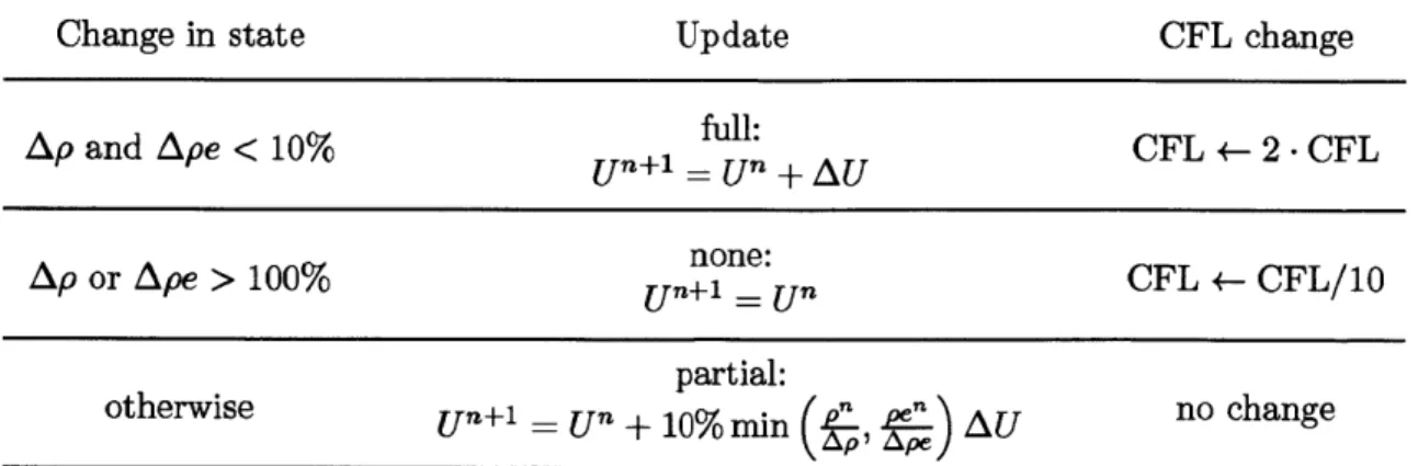
3.1 Summary of physicality check limits on the global CFL number. . . . . 46 3.2 Number of basis functions per element, nqf, for a given solution order and

reference element. . . . . 47 3.3 Summary of line-search limits on the global CFL number. . . . . 49 4.1 Table listing the information that is stored to define the different zerod objects. 54 4.2 Table listing the relevant information that is stored to define the different

oned objects. . . . . 55 4.3 Table comparing heat flux distribution errors calculated using sets of 484

randomly "speckled" points. All results are for p = 5. . . . . 63 4.4 Table comparing heat flux distribution errors calculated using sets of

ran-domly "speckled" points, distributed sampling points, and a canonical-cut grid. The Nquas for the "speckled" points is taken from the distributed sam-pling points to allow for the comparison between the methods. The results

areforp=5... ... 65

7.1 Summary of "cost" to generate the lift curve for the MDA airfoil using boundary-conforming and cut-cell meshes . . . .. . . . 163

Chapter 1

Introduction

1.1

Motivation

Computational fluid dynamics (CFD) methods have improved greatly over the past few decades, driven by the desire to perform more complex simulations. As Mavriplis et al. [88] describes, "While it is true that capabilities exist that are used successfully in every-day engineering calculations, radical advances in simulation capability are possible through the coupling of increased computational power with more capable algorithms." Controlling simulation accuracy is a primary issue for the application of CFD to increasingly complex problems.

A critical step in the application of CFD is mesh generation. Meshing is commonly performed by engineers who are required to make decisions about where increased mesh resolution is needed. CFD's dependence on human interaction is costly in terms of man hours and has the potential to introduce solution errors due to the mesh dependence of CFD solutions. In addition, this dependence on human interaction limits the automation that could be achieved with computational models. In 2007, following the third AIAA Drag Prediction Workshop (DPW-III) [1, 125], Mavriplis [85] used a generic wing-alone geometry

at Moo = 0.76, a = 0.50, and Re = 5 x 106 to demonstrate CFD's dependence on the initial mesh topology. Figure 1-1, taken from Mavriplis [85], shows the convergence of drag with mesh refinement for two families of meshes representing the same wing geometry. Both mesh families consist of four meshes and all the solutions were computed using the NSU3D code, an unstructured mesh Reynolds-averaged Navier-Stokes (RANS) solver [86, 87, 89].

The first set of meshes was generated at NASA Langley using the VGRID grid generation program [112], while the second set of meshes was generated independently at the Cessna Aircraft Company. Typical industry practice for an isolated wing problem is to use one to four million elements. However, as illustrated by Figure 1-1, even with an increase in refinement of an order of magnitude more than typical industry practice, the spread in the computed drag between the two meshes is approximately four drag counts. A Breguet range equation analysis demonstrates that a difference of one drag count for a long-range passenger jet corresponds to approximately four to eight passengers [44, 124]. Thus, the spread of four drag counts between the two mesh families is significant. Generating solutions to engineering-required accuracy from one tenth to one drag count is necessary for CFD to be a useful design tool [129]. 0.0212 0.0210 - Topology 1 , 0.0208 -0 0.0206- Topology 2 0.0204-0.6 0.8 1 1.2 h 2 -N-M _{x 10,}

Figure 1-1: Computed drag convergence for a wing-alone configuration at Moo = 0.76, a = 0.50, and Re = 5 x 106 with global mesh refinement taken from Mavriplis [85]. Convergence of drag is plotted for the refinement of two mesh families of the same wing geometry.

In addition to ensuring engineering-required error levels, improving the robustness of RANS solution algorithms is critical. Convergence to a steady state solution can be chal-lenging and tests the limits of a non-linear solver. Generally, while the linear systems are

poorly conditioned, the lack of robustness stems form the non-linearity of the problem. The convergence results of Bassi et al. [18], Figure 1-2, confirm the author's experience. Typically, in RANS simulations, residual convergence history is dominated by slow overall convergence and a lack of Newton convergence. The poor convergence tends to include spurious residual jumps where, over a single iteration, the residual norm will increase by over an order of magnitude. The residual jump is often followed by a period of residual decrease, but the process appears to arbitrarily repeat itself.

600 800 lieramtn Steps

Figure 1-2: Convergence history for p = 0 -+ 3 of RANS simulations of an

RAE2822 airfoil (Moo = 0.734, a = 2.79*, Rec = 6.5 x 106, 8,096 q = 3 quadrilateral elements) taken from Bassi et al.[18].

1.2

Objectives

Algorithm advances are required, in order to meet the demand for more complex CFD simulations. The objective of this work is to develop a reliable solution strategy that provides engineering-required accuracy for the two-dimensional RANS equations. To be reliable the strategy must be fully autonomous without requiring user interaction or detailed previous

knowledge about the flow to facilitate either adaptation or solver robustness. 1 To achieve the desired reliability and engineering-required accuracy, this work presents a solution strategy that incorporates a higher-order discretization, cut-cell meshes, output-based adaptation, and a line search based non-linear solver technique.

1.3

Solution Strategy Background

1.3.1

Higher-Order Method

For the last couple of decades, finite volume discretizations have been the industry standard for CFD in the aerospace industry. Complex simulations using finite volume discretization have been made possible through improvement in computational hardware and solution algorithms. However, traditional industrial finite volume schemes are second-order accurate, where a global uniform mesh refinement results in reduction of solution error by a factor of four, but an increase of eight in the number of degrees of freedom in three dimensions [881. Higher spatial accuracy may be obtained with fewer degrees of freedom by using a higher-order finite volume scheme, but higher-higher-order finite volume schemes based on reconstruction of the cell or nodal averages extend the numeric stencil and complicate the treatment of boundary conditions [102].

Higher-order finite element discretizations provide an alternative for achieving higher accuracy with fewer degrees of freedom than second-order schemes. This work uses the discontinuous Galerkin (DG) method. The DG method can maintain a compact nearest neighbor stencil (viewed element-wise), as the solution representation is discontinuous across elements and coupling comes only through face fluxes. Higher-order accuracy is obtained in the DG method by increasing the polynomial order used to represent the solution in each element.

The DG method was originally introduced for the neutron transport equation by Reed and Hill [114]. One of the first extensions to the original DG method was by Chavent and Salzano [27] who applied it to non-linear hyperbolic problems using Godunov's flux. Cockburn, Shu, and their co-authors were influential in expanding the use of the DG method.

'It is important to note that the user is still required to form a well posed problem applying proper boundary conditions and shock or turbulence models where applicable.

They combined DG spatial discretization with Runge-Kutta explicit time integration for non-linear hyperbolic problems [30-32, 34, 36]. Separately, Allmaras and Giles [4, 5] developed a second-order DG scheme for the Euler equations. This method is based on taking moments of the Euler equations as suggested by van Leer [122].

DG has also been extended to elliptic problems, beginning with interior penalty (IP) methods [7, 132]. More recently, Bassi and Rebay developed two methods (BR1 and BR2) [15, 16] and applied them to the Navier-Stokes equations. Similarly, Cockburn and Shu developed local discontinuous Galerkin (LDG) for convection-diffusion problems [33]. How-ever, LDG has an extended stencil when it is used for unstructured grid problems in multiple dimensions. The extended stencil led to the development of compact discontinuous Galerkin (CDG) by Peraire and Persson [107]. Rigorous frameworks for analyzing various DG meth-ods have been developed by numerous researchers including Arnold et al. [8] who presented a unified framework to analyze stability and convergence of DG schemes for elliptic problems. Other approaches have more recently been developed for elliptic problems [35, 106, 123, 131]. The DG method has additionally been applied to the RANS equations. Specifically, Bassi and Rebay [14, 18] have successfully used the BR2 method for the RANS equations with a k-w turbulence model [133]. Nguyen et al. [94] used CDG for RANS with the Spalart-Allmaras (SA) turbulence model [118]. Since then, Landmann et al. [79], Burgess, Nastase, and Mavriplis [24], and Hartmann and Houston [65] have also applied variants of the DG discretization to the RANS equations. This work builds off the implementation of Oliver and Darmofal [96, 98, 100], which uses the BR2 method with the SA turbulence model for closure.

1.3.2

Output-Based Error Estimation and Adaptation

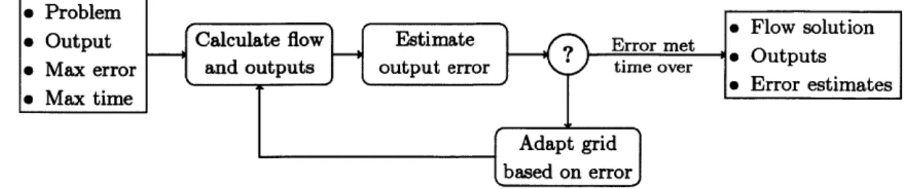
Output-based error estimation and adaptation autonomously reduces discretization error by estimating the error in a solution output and generating an improved mesh. Figure 1-3 shows an illustration of the adaptive framework. In this setting, a CFD user specifies a problem, an output of interest, a maximum allowable error, and a maximum run-time. From these inputs the adaptive strategy proceeds by (1) running a simulation on an existing (typically coarse) mesh, (2) computing an error estimate for the output of interest, and (3) determining whether the error tolerance or time constraint was met or if the mesh should be

Figure 1-3: Illustration of the autonomous output-based error estimation and adaptation strategy.

adapted and the process repeated. In the case where the mesh is adapted, the error estimate must be localized to identify regions where the mesh resolution requires improvement. The adaptation strategy is based on two elements: the output-based error estimate and the mechanics of changing the discretization to improve output error.

Error Estimate

Many methods exist for estimating the error in a solution. For instance, local error estimates can be performed by computing the difference between the current solution and a solution computed on a refined discretization, either from a refined mesh or increased solution order. This estimation strategy focuses on local solution errors and can be viewed similarly to feature-based adaptation where refinement requests are based on large local gradients. The local error estimation can fail in convection problems where small upstream errors can propagate and significantly change output evaluation [119]. For example, small errors can affect the location of boundary layer separation or a shock and lead to a significant change in outputs such as lift or drag.

The error estimation method used in this work is based on the Dual Weighted Residual (DWR) method from Becker and Rannacher [19, 20]. In the DWR method, the error in a solution output, such as lift or drag, is expressed in terms of weighted residuals. The weighted residuals are constructed using the dual problem and Galerkin orthogonality of the finite element discretization. The solution to the dual problem, the adjoint, relates local perturbations to an output of interest. For output-based error estimation the perturbations are the discretization error of the primal problem. The adjoint highlights aspects of the discretization which are most influential to the output of interest, thus it plays a central role in performing output-based error estimation. With the DWR method, asymptotically sharp

error estimates can be achieved by multiplying local residuals with the adjoint solution. Many researchers in the literature have applied the DWR method to the DG discretization with minor differences [47, 61, 63, 64, 67, 80, 84].

Extensions to the DWR method also appear in the literature. Pierce and Giles [54, 56, 111] presented the opportunity for improved output functional evaluation through error correction in the absence of Galerkin orthogonality. Venditti and Darmofal [128] were the first to apply an output-based error estimation and anisotropic adaptive method to the RANS equations. Their work concluded that for a standard finite volume scheme the output-based adaptive approach was superior in terms of reliability, accuracy in computed outputs, and computational efficiency relative to adaptive schemes based on feature detection.

Adaptation

Once an error estimate has been computed, the goal of adaptation is to modify the discretization to decrease the estimated error. There are three general adaptation options: h-adaptation, where the interpolation order remains fixed and the element sizes, h, are adjusted; p-adaptation, where the interpolation order, p, in elements with large error is in-creased to add resolution while the mesh remains unchanged [9, 84, 117]; or hp-adaptation, where both the interpolation order and the element size are changed [52, 53, 59, 60, 69, 119, 130]. All three of these adaptation strategies have strengths and weaknesses. p-adaptation is dependent on solution regularity. In the presence of solution discontinuities, higher-order in-terpolations demonstrate Gibbs phenomenon and p-adaptation will be ineffective. However, if sufficient solution smoothness is present, p-adaptation exhibits spectral convergence (in the limit of global increase in solution order). h-adaptation, though limited to polynomial

convergence, is particularly useful in shock or boundary layer cases where increased solution resolution is locally needed. The solution regularity of CFD problems in aerospace is lim-ited by singularities and singular perturbations. To achieve engineering required accuracy, resolution of the singular features is needed as opposed to high asymptotic convergence of the error. hp-adaptation would be the most effective adaptation procedure, but the decision between h and p refinement is not trivial.

This work depends on Riemannian metric based anisotropic h-adaptation to efficiently resolve features such as shocks, wakes, and boundary layers with arbitrary orientations. Global re-meshing of the simplex mesh is performed at each adaptation iteration. The

el-ement size requests in the adapted mesh are based on a fixed-fraction marking strategy. With fixed-fraction marking, refinement is requested for a fixed percentage of elements with the largest error while coarsening is requested for a percentage of the elements with the smallest error. The fixed-fraction marking strategy used in this work is distinct from tradi-tional fixed-fraction adaptation based on hierarchical subdivision of elements. The marking strategy is a means to redistribute element sizes within a requested metric field but does not cause a discrete change in the degrees of freedom.

One of the advantages of h-adaptation is it allows for straightforward anisotropic mesh refinement (anisotropic p-refinement is technically feasible but is not explored in this work). For anisotropic mesh indicators the solution Hessian of Mach number has been used by Venditti and Darmofal [126, 128] for second-order schemes. For a second-order scheme aligning the anisotropic metric with the Hessian equidistributes the interpolation error in the principle metric directions. Fidkowski and Darmofal [47] generalized the Hessian-based analysis to higher-order schemes by basing the principle stretching directions of an element on the maximum p+1 derivative. A more direct approach to mesh adaptation has also been used for anisotropic mesh adaptation by selecting the local mesh refinement of a single element which results in the most competitive subdivision of that element in terms of reduction of the error estimate [26, 53, 68, 103, 120]. An additional method proposed by Leicht and Hartmann [80] uses the inter-element jumps inherent to the DG solution to indicate where anisotropic adaptation is required.

1.3.3

Cut-Cell Mesh Generation

Two details of the solution strategy described above motivate the use of cut-cell mesh gener-ation. The first motivation for cut cells comes from the use of a higher-order discretization, where boundary conditions must contain higher-order information about the geometries they represent. The second motivator for the cut-cell method is adaptation, which requires repeated, reliable, and autonomous mesh generation.

Mesh generation about complex three-dimensional shapes is difficult even for linear (i.e. planar-faced) elements, in particular when high anisotropy is desired near the surface to resolve boundary layers. Mesh generation for boundary layers is sufficiently difficult that many researchers have adopted a hybrid approach. The hybrid approach employs a fixed

curving only

---boundary surface

valid linear mesh

curving

with

cut-cell

elasticity

intersection

Figure 1-4: Diagram of the options for converting a linear boundary

con-forming mesh to a mesh containing higher-order geometry

in-formation.

highly-anisotropic structured boundary layer mesh coupled to an unstructured mesh that fills

the computational domain [83, 104, 105]. Even in cases where it is feasible to generate linear

boundary-conforming meshes, conversion to a higher-order curved-boundary surface may

push through an opposing face as shown in Figure 1-4. One practice to generate a

higher-order mesh, also shown in Figure 1-4, is to globally curve a linear boundary conforming mesh

with elasticity [95, 100, 110].

A method to tackle the problem of reliably generating meshes of complex geometries

with higher-order information is the cut-cell method, shown in Figure 1-4. Purvis and

Burkhalter [113] were the first to consider a cut-cell method for a finite volume discretization

of the full non-linear potential equations. Purvis and Burkhalter started with a structured

Cartesian mesh that did not conform to the geometry and simply "cut" the geometry out.

Cut cells allow the grid generation process to become automated, taking a process which

was previously human-time intensive and dominated the solution procedure and making it a

preprocessing step. While relieving the mesh generation process, the cut-cell method requires

an ability to discretize on the arbitrarily shaped cut cells. Purvis and Burkhalter's method

used rectangular/box shaped cells from which the geometry was cut out in a piecewise linear

fashion. Although the linear intersections did not provide higher-order geometry, Purvis and

Burkhalter laid the foundation for future work with Cartesian cut cells. The full potential equation was also solved using a Cartesian cut-cell method by Young et al.[137] in TRANAIR. Cart3D, a three-dimensional Cartesian solver for the Euler equations [3], is a current example of the benefits of adding robust cut-cell mesh generation to a flow solver. Cart3D is based on embedding boundaries into Cartesian hexahedral background meshes and has proven capable of handling very complex geometries, like in the space shuttle debris calcula-tions performed by Murman et al.[2]. Work by Nemec [91-93] has added adjoint-based error estimates and adaptive refinement, which has provided an automated solution procedure for the Euler equations. Along with Cart3D, Cartesian embedded mesh generation has been used extensively in the literature [28, 51, 70].

While providing a robust meshing algorithm, a Cartesian cut-cell mesh limits the achiev-able directions of anisotropy, making the discretization of arbitrarily-oriented shock waves, boundary layers, or wakes highly inefficient. An application of a Cartesian cut-cell method to the Euler equation for transonic and supersonic flows by Lahur and Nakamura [77, 78] demon-strates the ease in which adaptation can be performed with a Cartesian cut-cell method, yet also the inability for axis aligned anisotropic elements to align with arbitrarily-oriented shock waves. The simplex cut-cell method, introduced by Fidkowski and Darmofal [45-47], offers an autonomous route for generating computational meshes with high arbitrary anisotropy and curved geometry information. Combining the simplex cut-cell method with a higher-order discretization, like the DG method in this work, provides the necessary tools to solve viscous flows over complex geometries. Fidkowski demonstrated the ability of the simplex cut-cell method to solve Euler and Navier-Stokes flows in two dimensions and Euler flows in three dimensions. The method was also used to model a rotor in hover [90].

The cut-cell method is well suited to the DG discretization. DG allows for inter-element jumps of the solution so forming a continuous basis within the computational domain is not necessary. Due to the nature of the cutting procedure the resulting element shapes are arbitrary and the possibility exists for large jumps in element volume across a common face. In order to incorporate cut-cell meshes into a DG discretization, the capability is needed to represent solutions and integrate the residual on arbitrarily shaped elements.

1.4

Thesis Overview

The primary contributions of this work are the following:

* Development of the capability to reliably solve high Reynolds number two-dimensional RANS problems using a higher-order, adaptive, cut-cell method

" Quantification of the impact on solution efficiency (defined as accuracy per degree of freedom) in the transition from boundary-conforming elements to simplex cut cells on a wide range of aerospace problems including subsonic through supersonic conditions and complex geometries

" Analysis of the impact of small volume ratios on linear system conditioning and solution quality, particularly boundary output evaluation, to identify its root cause and develop a method based on the analysis to alleviate the consequences of small volume ratios

* Development of a line-search globalization technique based on the unsteady residual of a pseudo-transient evolution to improve the robustness of non-linear solvers

" Quantification of the impact of randomness on the algorithm for generating integration rules for cut elements and development of integration rules based on canonical shapes where applicable, while otherwise, improve the accuracy and robustness of the general algorithm for arbitrarily shaped elements

modification of the general algorithm for arbitrarily shaped elements

e Development of an adaptation strategy that is less dependent on solution regularity and poor error estimates in under-resolved meshes

There are four primary research groups working on adaptation and higher-order DG discretizations of the RANS equations: the ProjectX team here at MIT, the Hartmann led research group at DLR (the German Aerospace Center), the research group of Fidkowski at University of Michigan, and Bassi's research group at Universitd di Bergamo. The groups share the common ability to use the DG discretization to perform high-fidelity RANS sim-ulations, but have different methodologies. Currently, the other three research groups rely on hierarchical refinement of quadrilateral and hexahedral meshes. The contributions made

in this thesis have lead to the unique capability to solve the higher-order DG discretiza-tion of the RANS equadiscretiza-tions on unstructured meshes with simplex cut-cell based adaptadiscretiza-tion. The unstructured simplex meshes allow for arbitrarily oriented anisotropy to resolve all flow features uncovered by output-based adaptation, and the cut-cell method provides reliable higher-order geometry representation while decreasing the strain of mesh generation. The simplex meshes reduce simulation cost in terms of degrees of freedom compared to structured meshes for flows with arbitrarily oriented anisotropic features.

The two-dimensional, adaptive, cut-cell solution strategy presented in this thesis is used to examine the competitiveness of the cut-cell technique for RANS-SA problems before it is extended to three dimensions. To that end the decisions made to incorporate the cut-cell strategy into a DG solver are intended to be general and extendable to three dimensions. All the two-dimensional RANS-SA flow simulations presented in this thesis can be com-puted using globally curved boundary-conforming meshes, but they are used to quantify the difference in solution efficiency between cut-cell and boundary-conforming meshes. A concern with the simplex cut-cells technique based on linear background meshes was that the resolution of boundary layer features would be inefficient [45]. The results presented in Chapter 7 provide quantifiable evidence that linear cut-cell meshes can provide equivalent solution efficiency in comparison to boundary-conforming meshes at engineering-required accuracy. The high solution efficiency on the complex two-dimensional problems explored in this thesis provide a motivation for the extension to three dimensions where the true benefit of the cut-cell technique will facilitate the generation of higher-order meshes for complex geometries.

While the contributions have been made for the advancement of a solution strategy for RANS problems, the contributions are intended to be generally applicable to a wide range of problems resulting for the discretization of PDEs. This work relies on the discontinuous Galerkin finite element discretization of the RANS-SA equations presented in Chapter 2. Chapter 3 presents the development of a line-search globalization technique to improve the robustness of non-linear solvers based on pseudo-time continuation. Chapters 4 and 5 describe advancements made to the two-dimensional simplex cut-cell technique. Special attention is paid to the analysis of the impact of small volume ratios which result from the cut-cell method. Chapter 6 reviews the output-based error estimation and adaptation

method used in this work. The solution strategy is applied to a wide range of aerospace problems in Chapter 7. Finally, conclusions and ideas for future work are given in Chapter 8.

Chapter 2

Discretization of the RANS-SA

Equations

The chapter begins with a brief review of the Reynolds-averaged Navier-Stokes (RANS) equa-tions and the Spalart-Allmaras (SA) turbulence model in Secequa-tions 2.1 and 2.2. Section 2.3 shows the spatial discretization and the chapter concludes with Section 2.4, a summary of the shock capturing employed in this work.

2.1

The RANS Equations

The solution to the compressible Navier-Stokes equations for turbulent flows of engineering interest poses a prohibitively expensive problem due to the large range of temporal and spatial scales present in the flows. It is common to solve the Reynolds-averaged Navier-Stokes (RANS) equations which govern the turbulent mean flow. The RANS equations are derived by averaging the Navier-Stokes equations. Favre averaging is used for compressible

flows. The form of the RANS equations in this work is [100] + a(Pi) = 0, (2.1) & ' 165 (9 _0Pi)+a(iit Ox L\ 3 Xk / [2(p,1+p/t)

(8-j

-

3

1P i+

Ui

+

ijI+

G~

a c,

+

+ a

64i2(pL+ p~t)

sij

1 O66(23

Oxj

Pr

Prt )

axj

3

where p denotes the density, ui are the velocity components, p is the pressure, e is internal energy, h is the enthalpy, T is the temperature, si, = , + is the strain-rate tensor, .s is the dynamic viscosity, pit is the dynamic eddy viscosity, Pr is the Prandtl number, Prt is the turbulent Prandtl number, d is the spatial dimension, and the summation on repeated indices is implied. The

(-)

(-)

The RANS equations, Equations (2.1) through (2.3), contain more unknowns than equa-tions requiring closure to solve the system. The remaining unknown, which cannot be computed, is pt. p1

t relates the mean flow viscous stresses to the stresses due to turbulent fluctuations. The Spalart-Allmaras turbulence model, described in Section 2.2, closes the RANS system of equations.

To simplify the notation for the remainder of this thesis, the

(-)

(-)

2.2

The SA Turbulence Model

A turbulence model is necessary, in order to close the RANS equations. This work relies on the Spalart-Allmaras (SA) turbulence model [118]. The specific form of the model is based off the work of Oliver [100]. Oliver incorporated modifications to the original SA model to

alleviate issues of negative P, the working variable for the SA equation. The SA equation is particularly susceptible to negative P when employing a higher-order discretizations.

The SA model was selected because of its wide use in the aerospace industry and high regard. The model has accurately simulated attached and mildly separated aerodynamic flows [25, 38, 57, 134].

The model takes the form of a PDE for P, which is algebraically related to the eddy viscosity, pt. The eddy viscosity is given by

At P~fv1 F1 > 0 0 F1 < 0.

where

x

Al 3 +,7 X v

and v = p/p is the kinematic viscosity. Then, pf, is governed by

(99

8

6~

- (pP) + (puj P) =P - D

+- ---

-

+cbsp,

(2.4)

0- _OxJ '5xj + x

Ox

where the diffusion constant, 7, is

77 =

{

(i

x

),

(1+ X+ IX2) X .

the production term, P, is

1COpP, _{X 0}

(2.6) cb1Sp19n, X < 0,

the destruction term, D, is

D = CWif4P. 7

x

S is the magnitude of the vorticity, such that S+ S, _S>C 2S _(2.8) =

s+

S)

-c,

S,

fv2=1-

The remaining closure functions are

f

P fgX 2

gr=52d2' " + X2

where d is the distance to the nearest wall, Cbi = 0.1355, o- = 2/3, Cb2 0.622, K = 0.41,

Ci = Cb1/K 2 + (1 + Cb2)/a, Cw2 = 0.3, Cw3 = 2, col = 7.1, C,2 = 0.7, Cv3 = 0.9, and Prt = 0.9. In this work, only fully turbulent flows are considered. Hence, the laminar suppression and trip terms from the original SA model are omitted.

The form of the SA model shown in Equation (2.4) is modified from that in [118]. The first modification is the expansion of the original model to compressible flows. The remainder of the modifications handle the case of negative P. Though the exact solution to Equation (2.4) is for non-negative P, the discrete solution does not necessarily maintain this property. In fact the solution overshoots which can result from higher-order discretizations on an under-refined mesh, amplifying the occurrence of negative P values. Negative i/ values have a strong detrimental impact on the non-linear solution convergence. The complete analysis of the impact of negative i and the modifications to correct this behavior can be found in Oliver [100]. The only implemented change made from the model presented by Oliver is the default value of

fg..

2.3

Spatial Discretization

The RANS-SA equations can be expressed as a general conservation law given in strong form as

V-F(u)-V-,(u,Vu)=S(u,Vu) inn, (2.9)

where u = [p, pui, pE, pj]T is the conservative state vector, F is the inviscid flux, F, is the viscous flux, S is the source term, and Q is the physical domain.

The discontinuous Galerkin finite element method takes the strong form of the conser-vation laws in Equation (2.9) and derives a weak form. The domain, Q, is represented by Th, a triangulation of the domain into non-overlapping elements K, where n = UR and srin ,g = 0, i $

j.

ri

Vh = {v E [L(Q)]' I V O

f,

where r is the dimension of the state vector, PP denotes the space of polynomials of order p on the reference element Krefs, and f, denotes the mapping from the reference element to physical space for the element r. The specific mapping,

f,,

To generate the weak form of the governing equations Equation (2.9) is weighted by a test function, vh _{E Vh, and integrated by parts. The weak problem is: find uh(-, t) E VhP} such that

Rh(uh, vI) = 0, Vvh E V , (2.10)

where