Adaptive Matched Field Processing
in an Uncertain Propagation
Environment
RLE Technical Report No. 567
James C. Preisig
January 1992
Research Laboratory of Electronics Massachusetts Institute of Technology Cambridge, Massachusetts 02139-4307
This work was supported in part by the Defense Advanced Research Projects Agency moni-tored by the Office of Naval Research under Grant N00014-89-J-1489, in part by the Office of Naval Research under Grant N00014-91-J-1628, in part by the National Science Foundation un-der Grant MIP 87-14969, in part by a National Science Foundation Graduate Fellowship, and in part by a General Electric Foundation Graduate Fellowship in Electrical Engineering.
Adaptive Matched Field Processing in an Uncertain
Propagation Environment
by
JAMES CALVIN PREISIG
Submitted in partial fulfillment of the requirements for the degree of
Doctor of Philosophy at the
MASSACHUSETTS INSTITUTE OF TECHNOLOGY and the
WOODS HOLE OCEANOGRAPHIC INSTITUTION January 1992
Abstract
Adaptive array processing algorithms have achieved widespread use because they are very effective at rejecting unwanted signals (i.e., controlling sidelobe levels) and in general have very good resolution (i.e., have narrow mainlobes). However, many adaptive high-resolution array processing algorithms suffer a significant degradation in performance in the presence of environmental mismatch. This sensitivity to envi-ronmental mismatch is of particular concern in problems such as long-range acoustic array processing in the ocean where the array processor's knowledge of the propaga-tion characteristics of the ocean is imperfect. An Adaptive Minmax Matched Field Processor has been developed which combines adaptive matched field processing and minmax approximation techniques to achieve the effective interference rejection char-acteristic of adaptive processors while limiting the sensitivity of the processor to environmental mismatch.
The derivation of the algorithm is carried out within the framework of minmax signal processing. The optimal array weights are those which minimize the maximum conditional mean squared estimation error at the output of a linear weight-and-sum beamformer. The error is conditioned on the propagation characteristics of the envi-ronment and the maximum is evaluated over the range of envienvi-ronmental conditions in which the processor is expected to operate. The theorems developed using this frame-work characterize the solutions to the minmax array weight problem, and relate the optimal minmax array weights to the solution to a particular type of Wiener filtering problem. This relationship makes possible the development of an efficient algorithm for calculating the optimal minmax array weights and the associated estimate of the
signal power emitted by a source at the array focal point. An important feature of this algorithm is that it is guarenteed to converge to an exact solution for the array weights and estimated signal power in a finite number of iterations.
The Adaptive Minmax Matched Field Processor can also be interpreted as a two-stage Minimum Variance Distortionless Response (MVDR) Matched Field Processor. The first stage of this processor generates an estimate of the replica vector of the signal emitted by a source at the array focal point, and the second stage is a traditional MVDR Matched Field Processor implemented using the estimate of the signal replica vector.
Computer simulations using several environmental models and types of environ-mental uncertainty have shown that the resolution and interference rejection capabil-ity of the Adaptive Minmax Matched Field Processor is close to that of a traditional MVDR Matched Field Processor which has perfect knowledge of the characteristics of the propagation environment and far exceeds that of the Bartlett Matched Field Processor. In addition, the simulations show that the Adaptive Minmax Matched Field Processor is able to maintain it's accuracy, resolution and interference rejection capability when it's knowledge of the environment is only approximate, and is there-fore much less sensitive to environmental mismatch than is the traditional MVDR Matched Field Processor.
Thesis Supervisor: Alan V. Oppenheim
Title: Distinquished Professor of Electrical Engineering
Thesis Supervisor: Arthur B. Baggeroer
Acknowledgments
While the completion of a doctorate is looked upon as an individual accomplishment, it is rarely accomplished without the help of a significant cast of supporting charac-ters. Such is the case here, for it has been the friendship, guidance, and support of many people that has helped make the last six years some of the most exciting and stimulating of my life and have help me through the times when things got tough.
Over the past several years, Al Oppenheim has been a source of inspiration and stimulation, has tolerated my often unhealthy addiction to bicycle racing, and deftly alternated between providing the encouragement and critical evaluation which I needed. His guidance and friendship has helped me grow both professionally and personally. Art Baggeroer has similarly taken the time and effort to push me to de-velop more fully in my work over the past few years. For their concern, caring and effort, I am eternally grateful.
I would also like to thank Udi Weinstein, Bruce Musicus and Rob Freund for the time and friendship which they have freely given to help me both technically and personally in the past years. Henrik Schmidt has also provided much help with his constant feedback on acoustics issues and his continual help with using SAFARI in doing my work.
All my colleagues in the Digital Signal Processing Group, past and present, have been intrumental in making the last three years fun and challenging. Particular among these have been Greg Wornell, who has ridden with me on this roller coaster for the last six years and has been an accomplice in creating an unholy mess in my kitchen on many occasions; and Steve Isabelle, who, as an honorary member of TEAM THESIS 91, tolerated far more repetitions of the music of the Nylons and of Andrew Lloyd Webber than was reasonable. Special thanks also go to John Buck, Andy Singer, and Giovanni Aliberti who have patiently answered so many of my dumb computer questions that they must be convinced (rightly so) that I am a hopeless case when it comes to computer system management. My other friends including Jim and Carol Bowen, John and Dana Richardson, Josko and Liz Catipovic, and all my cohorts in the world of bicycle racing have been constant sources of friendship and excitement and have helped me keep the world in a little better perspective through all of this. And finally, the love and understanding of my family has been the pillar of support which has kept me upright over the years. Without them, none of this would have happened.
Financially, I have relied upon the generousity of others to keep me fed and in school here at MIT and WHOI. For their support, I would like to thank the National Science Foundation, the General Electric Foundation, the Office of Naval Research, the Defense Advanced Research Projects Agency, and the Woods Hole Oceanographic Institution.
To all of you, and to all of the many people who are not specifically listed above but who have been there and given of themselves whenever I needed their help and friendship, I say thanks. You have helped make it a wonderful 6 years.
Contents
1 Introduction 11
1.1 Linear, Adaptive, and Matched Field Processing ... . 13
1.2 The Signal Replica Vector ... ... . 15
1.3 Array Processor Performance in Uncertain Propagation Environments 17 2 Minmax Array Processing 21 2.1 The Minmax Signal Processing Framework ... 21
2.2 The Adaptive Minmax Matched Field Processor ... . 26
2.2.1 Signal Model ... 26
2.2.2 Processor Structure ... ... . 29
2.2.3 The Minmax Array Weight Problem . . . 31
2.2.4 The Minmax Array Processing Algorithm ... . 33
2.3 Solution of the Minmax Problem ... . 36
2.3.1 Characterization of w_.pt(f,z, , ') ... 2 37 2.3.2 The Least Favorable PMF Random Parameter Framework . 39 2.3.3 Solving for the Least Favorable PMF ... . 43
2.3.4 Least Favorable PMF form of the Array Processing Algorithm 48 2.4 Minmax Estimation Error Bounds . . . 48
3 Analysis and Interpretation of the Adaptive Minmax Matched Field Processor 53 3.1 MVDR Interpretation of the Adaptive Minmax Matched Field Processor 54 3.1.1 The Two-Stage MVDR Matched Field Processor ... . 55
3.1.2 Analysis of the Two Stage MVDR Matched Field Processor . 56 3.1.3 Replica Norm Considerations and a Normalization Modification 61 3.1.4 The Range and Sampling of the Environmental Parameter Set · 64 3.2 Numerical Analysis of the Adaptive Minmax Matched Field Processor 69 3.2.1 The Deterministic Ideal Waveguide ... . 70
3.2.2 The Arctic Ocean ... . 89
3.2.3 The Random Ideal Waveguide ... 105
3.3 Algorithm Complexity ... 116
4 Matched Field Calculation of the Signal Replica Vector 123 4.1 The Spatial/Temporal Cross-Correlation Function ... . 124
4.2 Ray Approximation ... 126
4.3 Normal Mode Approximation ... 137 4.4 Numerical Solution of the Wave Equation ... 144
5 Conclusions and Future Work 147
A Proofs for General Minmax Problems 151
List of Figures
2-1 The Minmax Signal Processor ... 22
2-2 Non-Optimal Solution. w =w, ... ... . 27
2-3 Optimal Solution: w =w ... 28
2-4 Array Processor Structure . . . .. 31
2-5 The MVDR Processor Bank ... 34
2-6 Conditional Mean-Squared Estimation Error ... ... . 42
3-1 The Two-Stage MVDR Matched Field Processor ... ... . 54
3-2 The Convex Hull of Replicas with Different Norms . ... 62
3-3 The Convex Hull of Replicas with Unit Norms ... 63
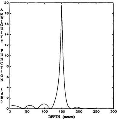
3-4 Ambiguity Function for the MVDR Processor: SNR = 10 dB Assumed Ocean Depth = 290 meters ... 74
3-5 Ambiguity Function for the MVDR Processor: SNR = 10 dB Assumed Ocean Depth = 310 meters ... 75
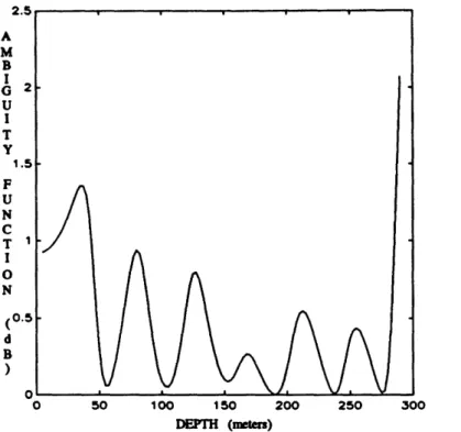
3-6 Ambiguity Function for the Bartlett Processor: SNR = 10 dB Assumed Ocean Depth = 290 meters ... 76
3-7 Ambiguity Function for the Bartlett Processor: SNR = 10 dB Assumed Ocean Depth = 310 meters ... 77
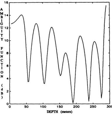
3-8 Ambiguity Function for the Minmax Processor: SNR = 10 dB Assumed Range of Ocean Depths = 290 to 310 meters ... ... . 78
3-9 Ambiguity Functions for SNR = 0 dB and Ocean Depth = 310 meters 79 3-10 Ambiguity Functions for the Minmax Processor: Two Sources . . . 82
3-11 Resolution Comparison for Different Processors . . . 83
3-12 Source Depth/Ocean Depth Response for Array Focal Point = 175 meters and Actual Ocean Depth = 290 meters ... 85
3-13 Source Depth/Ocean Depth Response for Array Focal Point = 175 meters and Actual Ocean Depth = 310 meters ... 86
3-14 Source Depth/Ocean Depth Response for Array Focal Point = 250 meters and Actual Ocean Depth = 290 meters ... 87
3-15 Source Depth/Ocean Depth Response for Array Focal Point = 250 meters and Actual Ocean Depth = 310 meters ... 88
3-16 Adaptive Minmax Processor Characteristics vs SNR ... . 90
3-17 Arctic Sound Speed Profile . . . .. 91
3-18 Ambiguity Function for the Matched MVDR Processor ... .. . 94
3-19 Ambiguity Function for the Mismatched MVDR Processor ... . 95
3-21 Ambiguity Function for the Adaptive Minmax Processor ... . 97
3-22 Array Gain vs SNR for Various Surface Sound Speeds ... . 98
3-23 cos2(qff,d; Sn(f)-1) vs SNR for Various Surface Sound Speeds . . 100
3-24 Least Favorable PMF for Various Actual Surface Sound Speeds . . . 101
3-25 Least Favorable PMFs (continued) ... 102
3-26 Peak Response Loss for Various Numbers of Environmental Samples. 104 3-27 Maximum Cross-Spectral Correlation Matrix Eigenvalues vs Modal Phase Decorrelation ... 110
3-28 Ambiguity Functions for = oo ... . 112
3-29 Ambiguity Functions for P = 2R ... . 113
3-30 Ambiguity Functions for = R . . . . 114
3-31 Ambiguity Functions for 8 : 0 ... 115
3-32 Ambiguity Functions for 8 = oo with redefined Replica Vector . . . 117
3-33 Ambiguity Functions for 8 = 2R with redefined Replica Vector . . . 118
3-34 Ambiguity Functions for P3 = R with redefined Replica Vector .... 119
3-35 Ambiguity Functions for 8 z 0 with redefined Replica Vector . . . . 120
4-1 Similar Rays ... . 134
4-2 Distinctly Different Rays ... 134
Chapter 1
Introduction
The signals received by spatial arrays of sensors are often composed of the sum of signals emitted by sources at different locations. In order to estimate the signal, or the parameters of the signal, emitted by a source at a particular location, the array processor must often separate that signal from the other signals which are received. This separation of signals based upon the location of the source is referred to as spatial filtering. Thus, the spatial filtering of signals received by an array of sensors to generate estimates of the parameters of the signals emitted by sources at locations of interest is an important operation in many array processing applications.
Array processors achieve spatial discrimination through filtering by exploiting the fact that the spatial characteristics of a propagating signal as received at an array of sensors depend upon the location of the source of the signal. However, the spatial characteristics of a propagating signal also depend upon the characteristics of the medium through which the signal is propagating. Therefore, if a processor has in-accurate or incomplete information concerning the characteristics of the propagation environment, it may be unable to determine the spatial characteristics which should be exhibited by a signal emitted by a source at the location of interest. In this case, the processor may have difficulty in accomplishing the spatial filtering necessary to estimate the parameters of the signal of interest. This work proposes an approach to array processing which yields a processor capable of operating with only approximate environmental information while at the same time achieving levels of spatial
discrim-ination which are close to those achieved by adaptive processors having accurate and detailed environmental information.
The remainder of this chapter contains general background information on array processing. Section 1.1 discusses general linear, adaptive, and matched field pro-cessing. Section 1.2 describes a parameterization of the spatial characteristics of propagating signals, which is useful for the class of algorithms considered herein. The problems which array processors exhibit when the environmental information is in-accurate, and possible approaches to developing processors which are able to operate effectively with inaccurate or imprecise information are reviewed in Section 1.3. This section also introduces the minmax signal processing approach, which is proposed herein to address the problem of array processing with only approximate environ-mental information.
The theoretical foundations of the minmax approach, based on the Minmax Char-acterization Theorm, are developed in Chapter 2. This theorem sets forth the neces-sary and sufficient conditions which must be met by any solution to a general class of minmax problems. The details of the proposed array processor, referred to as the Adaptive Minmax Matched Field Processor, are presented. A computationally effi-cient algorithm which is guaranteed to converge to an exact solution of the minmax optimization problem of interest is developed by exploiting the special structure im-posed on the solution by the Minmax Characterization Theorem. Finally, an approach to bounding the minmax performance achievable by any processor is proposed.
In Chapter 3, the structure imposed by the Minmax Characterization Theorem is again exploited to relate the Adaptive Minmax Matched Field Processor to Capon's Minimum Variance Distortionless Response (MVDR) Matched Field Processor [9, 11]. The relationship developed leads to a qualitative analysis of the processor. This anal-ysis motivates a small change to the algorithm developed in Chapter 2. A quantitative analysis of the algorithm based on results of numerical simulations is also presented. These numerical results are generated for both deterministic time-invariant and ran-dom time-varying propagation environments. The results for the latter case motivate another small change to the algorithm which is also detailed.
Chapter 4 addresses the problem of generating a priori estimates of the spa-tial/temporal characteristics of a propagating signal as a function of environmental conditions and source location. This chapter does not present original work. Instead, it presents results developed by others [29, 30, 31, 32, 33, 40, 41] on the propagation of signals through random media and outlines how this work can be applied to gen-erating estimates of the spatial/temporal signal characteristics. Finally, the results generated herein are summarized and future work is discussed in Chapter 5.
1.1
Linear, Adaptive, and Matched Field Processing
Many types of array processors either implicitly or explicitly incorporate a linear weight-and-sum beamformer to implement spatial filtering. This filtering allows the processor to discriminate among signals based upon the location of the source of the signals. Given an input y (the joint temporal/spatial filtering of the sampled vector time series y[n] will not be considered in this introduction), the output of a linear weight-and-sum beamformer is = why where w is the array weight vector, the superscript h denotes complex conjugate transpose (i.e., Hermitian), and i is an estimate of the signal emitted by a source at a location of interest.
Linear beamformers enjoy widespread use for several reasons. First, they generally have the lowest computational complexity of the available methods of implementing a spatial filter (given an N element array, the filtering operation is an X (N) opera-tion and, if required, the calculaopera-tion of the array weights to minimize a squared error criterion is often an O (N3) operation). Second, when the array weights are chosen to
minimize a mean-squared estimation error criterion, the solution for the optimal ar-ray weights is a convex quadratic minimization problem and is analytically tractable. Third, linear filtering preserves the actual time-series of the signal of interest which is important in many applications. Finally, when the received signal consists of the sum of a signal of interest and interfering signals,the spatial correlation of the inter-fering signals is different from that of the signal of interest, and the signal of interest is correlated across the aperture of the array, the linear beamformer is effective at
filtering out the interfering signals and generating an estimate of th signal of interest. Another class of array processors which enjoys widespread use it the adaptive array processor. Adaptive array processors use observations of, or information about, the signal, noise, and propagation environments to adjust the characteristics of the processor to minimize or maximize some performance criterion. The processors are able to efficiently use the degrees of freedom available to the processor to adjust to the environment in which the processor is operating. [6] The most widely-used type of adaptive processors are those incorporating adaptive linear beamformers [7, 8]. Two such examples are Capon's MVDR Processor [9] and the Applebaum Beamformer [10]. These processors use observations of the combined signal and noise environment to adaptively adjust the array weight vector to optimally pass the signal of interest through the filter and while controlling the sidelobes of the filter's spatial response to reject the interfering signals contained in the received signal. In order to distinguish between the signal emitted by a source at the location of interest from all other signals, the processor uses a priori estimates of the spatial characteristics of the signals of interest. These a priori estimates depend upon the manner in which the propagating signals are modeled.
Traditionally, array processors have modeled propagating signals as plane waves following a straight line path from the source to the array of sensors. This corresponds to an implicit model of the propagation medium as being homogeneous and infinite in extent and the source being far from the array. The propagation of acoustic waves through the ocean is not modeled accurately in this manner. Both the time-invariant and the time-varying temperature, salinity, and pressure structures of the ocean are spatially-variant. When coupled with the finite extent (principally the finite depth) of the oceans, these spatially-variant structures cause acoustic signals to propagate in a manner which deviates significantly from that predicted by the plane-wave model. This deviation has both adverse and advantageous consequences. The adverse consequence is that, if a plane-wave model is used by the processor, the spatial char-acteristics of the signal of interest may not match those estimated by the processor. In this situation, which is referred to as model mismatch, the processor may treat the
signal of interest as an interfering signal and attempt to reject it. A more detailed discussion of this problem is contained in Section 1.3. The advantageous consequence is that, if the processor uses a fairly accurate environmental and propagation model, it is possible to achieve source localization accuracies which far exceed those which are available in an infinte, homogeneous medium [11].
A class of processors which has been developed to take advantage of this improved accuracy and to eliminate the model mismatch problems caused by the use of the plane-wave model is referred to as the Matched Field Processor. First proposed in [12], these processors use fairly complete environmental and propagation models to make a priori estimates of the spatial structure of received signals as a function of environmental condition and source location. The processors use these spatial structure estimates to operate on the received sound field and generate estimates of signal parameters of interest. The spatial structure of the signal of interest is parameterized by the signal replica vector as defined in the following section.
1.2
The Signal Replica Vector
The signal replica vector is a parameterization of the spatial characteristics of a propagating signal as a function of the location of the source of the signal and the propagation characteristics of the medium. Traditionally, the signal replica vector is defined for a narrowband signal propagating through a time-invariant medium. In this case, the signal replica vector is, to within a complex scaling factor, a replica of the deterministic narrowband signal emitted by a source at the location z as received at the array of sensors. Thus, given that a source at the location z emits the complex exponential Aej27'ftand the medium is time-invariant, the signal received by the array
of sensors can be expressed as
where A is a complex random variable, (f, z,
)
is the signal replica vector, is a parameterization of the characteristics of the propagation environment and the receiving array (e.g., the sound speed profile, the depth of the ocean, the sensor locations, etc.), and B = cA for some complex constant c which depends on the signal attenuation and progagation delay between the source and the sensor array and the manner in which the replica vector in normalized. The signal replica vector is usually normalized so that its magnitude equals one.For this work, the signal replica vector is defined in a stochastic signal framework
as
(fz E[X(f
z)Xk(, z)
I ! 11E[Xk(f,z)X*(f,Z)
I
]
(.1)where Xk(f, z) is the discrete-time Fourier transform at the frequency f of the signal
emitted by a source at the location z as received at the kt h array sensor, X(f, _) is
the discrete-time Fourier transform of the same signal as received at the entire array of sensors, and the kth sensor is the reference sensor of the array. Thus, the signal replica vector is the normalized cross-correlation between the discrete-time Fourier transform of the signal of interest as received at the reference sensor and the same signal as received at the entire array of sensors. It is important to note that the signal replica vector is defined in terms of the propagating signal as received at the array of sensors. This new defintion is used for two reasons. First, it explicitly allows the parameterization of the spatial structure of a signal emitted by stochastic source and which propagates through a random medium. Second, this parameterization incorporates all of the the information concerning spatial structure of the signal of interest which can be exploited by a linear processor which is optimized to minimize a mean-squared error criterion.
When the source at the location z emits the complex exponential Aej2
wft
and themedium is time-invariant as described previously, the signal replica vector as defined in (1.1) is, to within a complex scaling factor, identical to the traditionally defined replica vector also described previously.
qk(f, _ ,) = 1. Another normalization convention is proposed in Subsection 3.1.3. A different definition of the replica vector is proposed in Subsection 3.2.3. This defi -tion is similar in concept to (1.1) in that it is based upon the spatial cross-correla-tion of the signal of interest and, in a time-invariant propagation environment, these defi-nitions are roughly equivalent. However, in a random time-varying medium, they are
different, and the definition proposed in Subsection 3.2.3 yields better results.
1.3
Array Processor Performance in Uncertain
Propagation Environments
As mentioned earlier, array processors exploit the fact that the spatial characteristics of a signal as received at an array of sensors depend on the location of the source of the signal in order to differentiate among signals emitted by sources at different locations. High resolution processors are able to discriminate among signals whose spatial characteristics, parameterized here by the signal replica vector, differ only slightly. While the ability to discriminate among signals whose replica vectors differ only slightly provides good spatial resolution, it also makes the processor sensitive to changes in the propagation characteristics of the environment. A small change in the characteristics of the propagation medium resulting in a small change in the signal replica vector, may cause the processor to inaccurately estimate the location of the source of the signal.
Adaptive processors, such as Capon's MVDR Processor [9], are particularly sen-sitive to inaccuarate or imprecise knowledge of the characteristics of the propagation environment (referred to as model mismatch). This sensitivity stems from the fact that, if the processor incorrectly calculates the signal replica vector, then the received signal emitted by a source at the location of interest will not be recognized as such. Consequently, the processor will attempt to reject (i.e., filter out) that signal. The sensitivity of various adaptive and non-adaptive processors to model mismatch has been analyzed extensively [13, 14, 15].
mismatch have been proposed. The most commonly proposed approach, which is applicable to linear processors, is to add an additional constraint to the array weight optimization problem which places an upper bound on the norm of the array weight vector. A survey of these methods is contained in [8]. The motivation for these approaches is that the sensitivity of a processor to spatially uncorrelated perturbations to the nominal spatial characteristics of a signal is proportional to the norm-squared of the array weight vector. A related approach, referred to as the Generalized Cross-Spectral Method [16], is to add a penalty function proportional to the norm-squared of the array weight vector to the criterion, which is minimized or maximized by the selection of the optimal array weight vector.
Another approach to reducing the sensitivity of linear processors to model mis-match is to constrain the response of the linear weight-and-sum beamformer over a range of environmental conditions. One example is the Multiple Constraints Method [17], which accomplishes this goal by placing equality constraints on the response of the beamformer at a number of locations surrounding the location of interest. Relying on the fact that the signal replica vector is a smooth function of both the source loca-tion and the environmental condiloca-tions, the equality constraints at different localoca-tions surrounding the location of interest also constrain the response of the beamformer at the location of interest for various environmental conditions which are close to the nominal environmental condition. A more direct approach using the multiple con-straints approach [18] places equality concon-straints on the response of the beamformer for a number of environmental conditions which result from small perturbations to a nominal environmental condition. A related approach [19] uses inequality constraints on the response of the processor to insure that for various environmental conditions, the actual response is within some tolerance factor of the desired response.
A third approach to reducing the sensitivity of array processors to model mis-match, which is not limited in applicability to linear beamformers, is the random environment approach. here, the environmental parameters are considered random parameters with known probability distributions. The array weight vector or the esti-mate of the signal parameters are chosen to mininimize or maximize a criterion which
is averaged over the possible values of the environmental parameters. A Maximum A Posteriori source location estimator utilizing this approach is proposed in [20].
There are several drawbacks to these approaches. First, the approaches using linear equality constraints lose one degree of freedom in the beamformer for each constraint. This level of reduction in degrees of freedom may not be necessary to accomplish the desired goal. Second, the selection of the response levels, the norm bounds, and the tolerance factors is, in general, an ad hoc procedure without clearly defined criteria. Finally, the processors developed using the random environment ap-proach may exhibit poor performance for particular sets of environmental conditions even though their average performance is good.
This work seeks to develop an array processor which exhibits the efficient use of degrees of freedom and the interference rejection capability characteristic of adaptive array processors, and the source localization capability characteristic of the matched field processors while operating with only approximate information about the prop-agation characteristics of the medium. The minmax signal processing approach is proposed to develop such a processor. The minmax approach requires that an error criterion which is a function of the environmental conditions as well as the processor characterists be defined. Using this criterion as a measure of processor performance, the maximum value of the criterion taken over a user-specified range of environmental parameters is minimized. If this is done in an adaptive manner, the processor should be able to efficiently use its degrees of freedom to improve the performance of the processor for the environmental conditions where the performance is most critical.
The use of the minmax approach to develop a processor which is insensitive to modeling uncertainties has been studied previously ([21] and references therein). How-ever, the signal processing techniques developed therein are not applicable to the prob-lem of achieving spatial discrimination in an uncertain propagation environment, and are not adaptive in the sense described in Subsetion 1.1. Therefore, the Adaptive Minmax Matched Field Processor described in Chapter 2 is proposed to achieve the goal of this work.
Chapter 2
Minmax Array Processing
For the reasons stated in Chapter 1, a minmax approach is used here to develop an adaptive array processor which is robust with respect to uncertainties in the prop-agation environment. Section 2.1 presents a general minmax framework for signal processing along with a characterization theorem for the solutions to a large class of minmax signal processing problems. Using this theorem as a basis, an algorithm for adaptive minmax matched field processing is developed in Section 2.2. Section 2.3 addresses the implementation of the Adaptive Minmax Matched Field Processor. A new algorithm is developed to solve a particular class of quadratic minmax problems which includes the minmax portion of the Adaptive Minmax Matched Field Proces-sor. This algorithm has the desirable property of being guaranteed to converge to an exact solution in a finite number of iterations. Finally, a new approach to the development of minmax estimation error bounds is proposed in Section 2.4.
2.1
The Minmax Signal Processing Framework
The framework in which the array processing algorithm described in Section 2.2 is developed is minmax signal processing. In general terms the framework addresses the problem of developing a processor whose worst-case performance evaluated over a given class and range of uncertainties is as favorable as possible. Specifically, let g(y, w) be a processor parameterized by the vector w which operates on an observed
X
xFigure 2.1: The Minmax Signal Processor
signal y to generate an estimate of some signal or parameter of interest x (Figure 2-1). The
(.)
symbol denotes an estimate of the variable over which it is positioned (e.g., i denotes an estimate of the vector X.). The set of allowable values for the parameter vector w is denoted by W. In the case where g(y, w) is a linear filter with N taps, the vector w could contain the filter weights and W could be the space of N-dimensional complex numbers CN.The parameters which govern the relationship between the observed signal y and the signal or parameter of interest x are referred to as the environmental parameters and denoted by the vector _. In the context of array processing problems where y is the received signal and x is a particular signal of interest, the vector 0 could contain the location of the array sensors or the phase, gain, and directional characteristics of those sensors. It could also contain a parameterization of the interfering signals or the characteristics of the propagation medium. The ability of any particular processor as determined by the choice of w to estimate x depends upon the particular envi-ronmental condition under which the processor operates. Thus, a particular value of w which yields good processor performance under one environmental condition may yield very poor performance under another environmental condition. A real valued error function e(w, _) is used as a figure of merit to evaluate the performance of any particular processor operating under any particular environmental condition.
If the processor has perfect knowledge of the environmental conditions (e.g., - = 0), then the processor parameters can be chosen to minimize e(w, ). However, in many situations the processor does not have perfect knowledge of the environmen-tal conditions under which it must operate, but instead knows only that the uncertain environmental parameter _ falls within some range denoted by the set . The
cessor should then be designed to operate over this entire range.
As discussed in Section 1.3, one possible approach to designing the processor to operate over 4 is to treat , as a random parameter with an assigned pdf (probability distribution function) pO and then select w to minimize the average value of c(w, _) taken over v with respect to p_. That is,
w_t = arg min/ P0(0o) (w, O) dO MwEW - -0
However, this approach requires that a pdf be explicitly assigned to , and does not necessarily solve the problem of the processor performance being very poor for particular environmental conditions under which it may have to operate.
The minmax signal processing framework makes it possible to avoid these prob-lems when selecting w by treating , as a nonrandom parameter. Then, under the assumptions that e(w, 4) is a continuous function of , for every w E W and is a compact set contained in a metric space, the worst-case performance of the processor over the range of the environmental parameters is defined as
A( max (w, ).
A(w) is referred to as the extremal value for the processor parameter vector w. The optimal minmax processor parameter vector is defined as that which minimizes this extremal value. Mathematically, this is stated as
_.pt= arg mlin A(w) = arg min max e(w, 4).
EW w EW EO'
As in any optimization problem, the specification of the necessary conditions which must be met by the optimal solution and the sufficient conditions which guarantee that a solution is optimal are of central importance. The specification of such conditions for minmax optimization problems requires the definition of extremal points, extremal point sets, the convex hull of a set of points, and the gradient operator. An extremal point is any environmental point contained in 4 at which the error function e(w,
4)
achieves the extremal value A(w). The extremal point set, denoted by M(w), is the set of all extremal points. That is,
M(w)_{+E
·I
6(w,
)
=Given any set of points A contained in a metric space S, the convex hull of the set A in S, denoted by
X
(A), consists of all points s E S which can be expressed as the convex combination of the points a E A. That is,X(A) = {sES13J>O, a.EA, and piCR, for i=l,...,J
J J
s.t. Pi > i = l,...,J, Epi = and s=Zpia}
i=l i=1
A final required definition is that of the gradient operator. Let (w, 0) be any real valued scalar function of the vectors w and _. Then the gradient operator of e with respect to w is any vector function of w and _, denoted by Vwe (w, ), which is continuous with respect to w and and for which the following is true: There exists a real, positive scalar constant k such that for any particular processor pa-rameter vector (o) and environmental condition (i), the incremental change in e
corresponding to an incremental change in w away from w, denoted by
6w,
is equal to k < V (,o, w >, where < , > denotes the inner product. A formal state-ment of this definition is contained in Appendix A. The definition of the gradient as a vector of partial derivatives is not used because the error function used later in this chapter is not differentiable with respect to the elements of the complex vector w.Given the preceding definitions, the following Minmax Characterization Theorem, which is a generalization of that given in Chapter 6 of [1] for the case of minmax approximation with differentiable functions, states the conditions which characterize the optimal solution to a general class of minmax problems.
Theorem 1 Let be a compact set contained in a metric space denoted by , W be an open set of a Euclidian metric space denoted by E, e: W x - R be a continuous function on both W and for which, at each w E W, a directional derivative with respect to w can be defined on ,
and V"s (wI ) be the gradient of e with respect to w. Then a necessary condition for w E W to be a solution to the following minmax problem
wopt = argmin max e(w,),
wEW EO
is that
0 E
( V, (.)|
EM(,w)})
If, in addition, e is a convex function of w and W is a convex set, this condition is a necessary and sufficient condition for w. E W to be the solution to the stated minmax problem.
A proof of this theorem is contained in Appendix A. This theorem states that a necessary (and sufficient if e is convex on W and W is itself convex) condition for the optimality of w.o is that the origin, denoted by Q, is contained in the convex hull of the set of gradients of e with respect to w evaluated at the extremal points of e(w, ).
The following example may be useful to clarify the definitions and the concepts introduced thus far and to provide an intuitive interpretation of the Minmax Char-acterization Theorem.
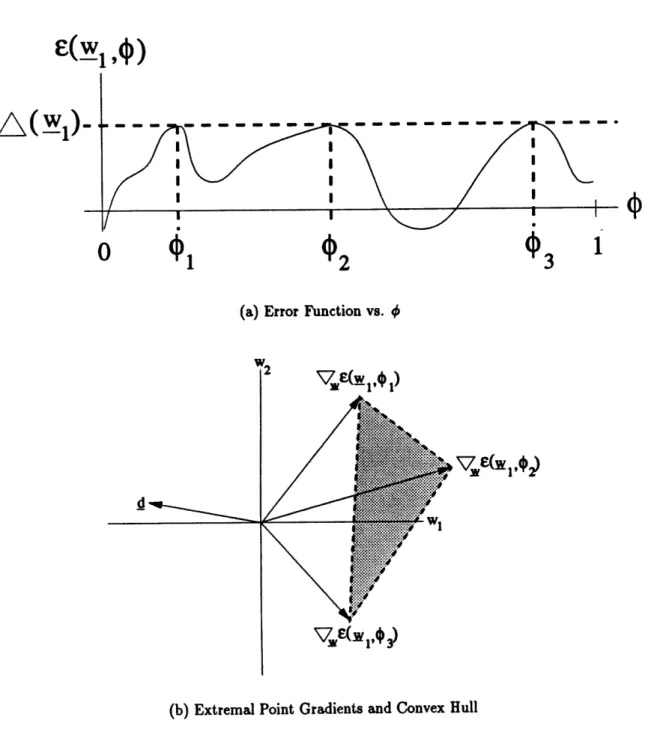
Example: Assume that w is a two-dimensional real vector, W = R22,
is a real scalar variable, ~ is the closed interval between zero and one (i.e.
=
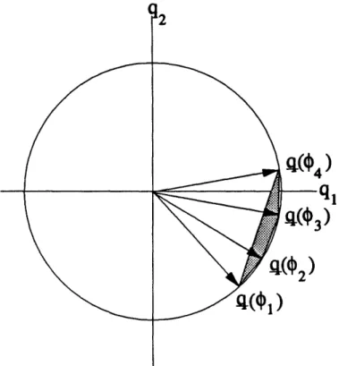
[0, 1]), and (w, d) is a real-valued scalar function which is convex with respect to w for all and continuous with respect to .For some i,, Figure 2-2a shows the error function plotted as a function of with the extremal value A(_) and the extremal point set M(g,) = {1l, 2, 03} labeled. The gradients of e with respect to w evaluated at
w and each of the three extremal points are shown in Figure 2-2b. The convex hull of this set of vectors is the shaded region. The origin is not in this convex hull and therefore wA, is not an optimal solution. This can be seen by noting that, if we can choose a direction vector such as d for which dtV (l,
Xi)
< 0 for i = 1, 2, 3, then the initial change in e evaluated at each of the extremal points will be negative as we move away from wl in the direction of d. Since the value of is simultaneously reduced at each of the extremal points as we move away from wl, the extremal value of e will be reduced as we move away fromwl
and thereforewl
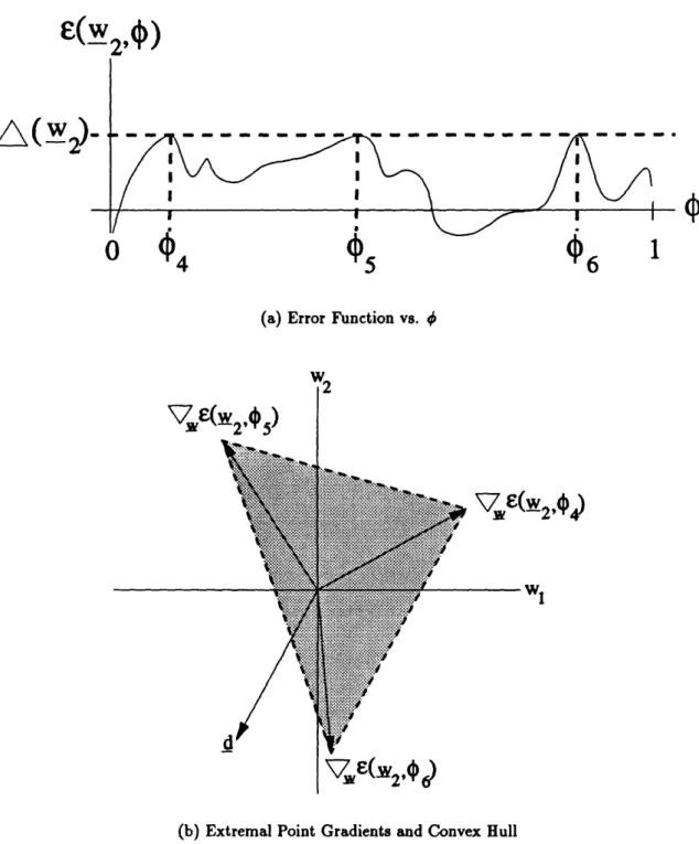
cannot be an optimal solution.For some w2, Figure 2-3a shows the error function plotted as a function of with the extremal value A(w2) and the extremal point set M(w2) =
{4, d5, 6} labeled. The gradients of e with respect to w evaluated
at w2 and each of the three extremal points are shown in Figure 2-3b with the convex hull denoted as before. In this case, the origin is in the
convex hull and therefore w is an optimal solution. This can be seen by noting that, for any direction vector such as d which we choose, the
inner product dtV,e (wi, O) will be greater than zero for at least one
of the three gradient vectors (in the case shown, dtV,,e (, 6) > 0). Therefore, as we move away from w2 in any direction d, the initial change in e evaluated at one or more of the extremal points will be positive. Since the value of e increases at one or more of the extremal points as we move away from _2, the extremal value of e will be increased as we move away
from w2. Therefore, w2 is a locally optimal solution. However, since e is
a convex function of w for all , ti(w) is also a convex funtion of w. (See Lemma A.2 in Appendix A). Therefore, w2 is a globally optimal solution.
2.2
The Adaptive Minmax Matched Field Processor
2.2.1
Signal Model
The Adaptive Minmax Matched Field Processor takes as its input the signal received by an array of sensors which has been low-pass filtered to prevent frequency domain aliasing and then sampled. This input is denoted by the vector time series y[m]. This input signal is assumed to be the sum of propagating background noise generated by spatial spread sources, such as, breaking surface waves, sensor noise which is assumed to be spatially white, and propagating signals generated by spatially-discrete point sources such as marine mammals, ships, etc.. xrm, z] denotes the time sampled received signal which was emitted by a point source at the spatial location z. n[m] denotes the sum of the sensor noise and the received propagating background noise. It is assumed that n[m] and x[m, z] are uncorrelated zero mean wide-sense stationary
random processes for each z and that _[m, _] and x[m, z2] are uncorrelated for any
two source locations z1
#
_2. Thus, y[m] is a zero mean random process representedby
y[m] = n[m] + [m
z_
The modeling of x[m, j as a zero mean random process can include a signal emitted by a stochastic source propagating through either a deterministic or a random environment, or a signal emitted by a deterministic source propagating through a
E,(wi
)
0
{1
{2
¢31
(a) Error Function vs.
W1
(b) Extremal Point Gradients and Convex Hull
Figure 2-2: Non-Optimal Solution: w = l d
0
I)4¢5
(a) Error Function vs. b
7
e(w
2,
5)
ffi
:: .':::e..':::;
d
7w
(w24pd
(b) Extremal Point Gradients and Convex Hull
Figure 2-3: Optimal Solution: w = 2
,(W
2
)
1
C-w2,e
4)
wl 1A(-w)
random environment.
2.2.2
Processor Structure
The Adaptive Minmax Matched Field Processor was developed to achieve the effective sidelobe control which is characteristic of adaptive processors such as Capon's MVDR Processor [9], and the improvement in spatial resolution provided by matched field processing techniques such as those presented in [11], without exhibiting the extreme sensitivity to mismatch in the estimation of the characteristics of the propagation environment which is exhibited by these algorithms and techniques [13, 17]. The quantity estimated by the processor is the average power in a selected frequency component of the signal emitted by a point source at a location of interest as received at one array sensor (the reference sensor). The location of interest is referred to as the array focal point. The signal emitted by a point source at the array focal point and received at the reference sensor is referred to as the desired signal and denoted
by xk[m, z]. Here the kth sensor is the reference sensor and z is the array focal point.
Unlike the case of traditional array processors, the desired signal is not the signal as emitted by a source at the array focal point. Instead, the desired signal is the signal emitted by a source at the array focal point as received at the reference sensor. The array focal point can be swept through space and the selected frequency can be swept through the frequency spectrum to generate an estimate of the average power in the desired signal as a function of spatial location and temporal frequency. This estimate is denoted by o2(f, z).
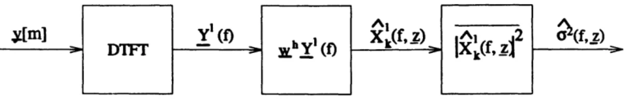
Conceptually, the processor which generates this estimate consists of three mod-ules (Figure 2-4). The first module divides the time-sampled signal received by the ar-ray y[m] into segments M samples in length which may be overlapping, and computes the vector discrete-time Fourier transform of each segment at the selected frequency
M-1
Y_(f) =
E
y[m]e-J2 am=O
I indicates the segment number, y'[m] is the mth sample of the Ith segment, and At
is the sampling period. Here, f is the frequency expressed in cycles per second which satisfies [ f 1< . f is not the normalized frequency expressed in cycles per sample
which satisfies f 1 . The linearity of the Fourier transform yields
Y'(f
f
) +
L(f)
where the summation is over the locations of the point sources. The transformed
seg-ments are known as "snapshots" and Xt(f, _) denotes the snapshot of the Ithsegment of x[m, _]. Yi(f) denotes the discrete-time Fourier transform of the Ih segment of
the signal received by the it array sensor. In effect, the first module is a temporal filter which selects the frequency component of interest in the received signal.
The snapshots of the received signal are the inputs to the second module which is a linear weight-and-sum beamformer. This beamformer computes an estimate of the Fourier transform of the Ith segment of the desired signal using
Xlk (f, ) = whyl (f)
where w is the array weight vector. The beamformer is a spatial filter which attempts to pass only the desired signal (i.e., that which was emitted by a source at the array focal point z) while rejecting all other signals received by the array sensors. The final module computes an estimate of the average power in the desired signal. The overbar indicates the sample mean taken over all 1. That is, if L is the number of segments
used in estimating
a
2(f, z), then1L
&2(f, z) = E .X I (fz)12·
While this structure is the same as that used by many array processors such as Capon's MVDR Processor, the unique feature of this processor is the manner in which the array weight vector w is calculated. For this processor, the array weight vector is the solution to a minmax optimization problem where the error e is a measure of the spatial filter's ability to pass the desired signal without distortion while rejecting the
Figure 2-4: Array Processor Structure interfering signals in a given propagation environment.
2.2.3
The Minmax Array Weight Problem
For any particular array focal point, frequency, array weight vector, and propagation environment, the error function for the Adaptive Minmax Matched Field Processor is the a priori mean-squared error in the estimation of Xk(f,_) conditioned on the characteristics of the propagation environment. That is
e(f,z,w, i) = E[l Xk(f,z)
-,f,j)
121 ij (2.1) = E[I X,(f,_) - wh Y(f) 12I
~J,where the characteristics of the propagation environment are parameterized by the vector _.
For a given array focal point and frequency, the optimal array weights are defined as
w.t(fz) = arg min maxe (f,z,w,), (2.2)
!ECCN E
where N is the number of array sensors and is the user specified range of the environmental parameters over which the processor must operate.
Under the assumption stated earlier that the desired signal and the interfering signals are uncorrelated, (2.1) can be rewritten as
(f,z,w_,) = E[Xk(f,z)Xk(f,&) - (2.3)
2 Real(E[X(f,)Xk(f, ) I jh w) + wh E[Y(f)y(f)h I ,
where the superscript * denotes complex conjugate.
The expectation in the last term of (2.3) is the cross-spectral correlation matrix of the received signal conditioned on the environmental parameter _. The cross-spectral correlation matrix is the parameterization used by the processor to characterize the spatial structure of the total signal field, and it is the input to the processor which enables the processor to adapt to reject unwanted signals. Here, the matrix will not be treated as a function of the particular environmental conditions or the characteristics of any particular propagating signal. Instead it wil be treated as a property of the total signal field. Therefore, the conditioning of the expectation in the last term of (2.3) is dropped and the actual ensemble cross-spectral correlation matrix, S(f), is used. In most cases, this ensemble cross-spectral correlation matrix is unknown to the processor. Therefore, the sample cross-spectral correlation matrix given by
S(f)
_ 1Z=a
yl(f)yl(f)h will be substituted for S(f). Nothing in the derivation ofthe algorithm in the remainder of this chapter depends upon this substitution. The expectation in the second term of (2.3) can be expressed as
EX* (E[X(f,z)X*(f,
z)
I
] E[Xk(fz)X~(fz)I
_]E[Xk(f,z)Xk*(fz)
i'
The quotient is the signal replica vector defined in Section 1.2 asA E[X(f, )Xk(f,_z) I _]
f, Z E[Xk(f, )Xk(f, z)
I J'
Therefore, the second term can be expressed as
2 E[Xk(f, z)Xk(f, z) I ]Real(qh(f, z, ) w) (2.4)
The signal replica vector in this factorization is the means by which the a priori model of the dependence of the desired signal's spatial characteristics on the environmental conditions is incorporated into the processor.
The expression E[Xk(f, z)Xk(f, z) I ] appears in the first term of (2.3) and, as
expression is the conditional average power in the desired signal, and will be replaced
by the actual average power in the desired signal 2(f,z) E[Xk(f,)X*(f,)].
Given the factorization and the substitutions detailed above, the error criterion can be expressed as
e(f,z ,w,,o' 2(f,z )) = 2(f,z) - 22 (f,I)Real(qh(f,z,) w) + wh
(f)
w,
(2.5)
where the dependence of the error on the average power in the desired signal is explicitly shown.
The optimal array weights minimize the maximum value of this error taken over the operating range of the environmental parameters. Conceptually, they can be considered those of a data-adaptive Wiener filter which is robust with respect to changes in the spatial correlation of the signal to be estimated.
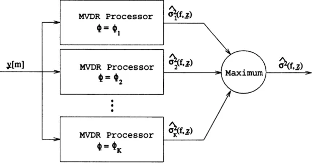
The Adaptive Minmax Processor described in this subsection can also be inter-preted as an efficient implementation of a bank of MVDR Matched Field Processors, each using a different assumed value of the environmental parameter vector () and therefore of the signal replica vector (q(f, _, _)) (Figure 2-5). The range of assumed values of is the range of environmental conditions over which the processor is de-signed to operate. The Adaptive Minmax Processor output is the output of the MVDR Processor with the largest estimated average power. The derivation of this interpretation is detailed in Section 3.1 where the processor bank interpretation is equivalent to the Two-Stage MVDR Matched Field Processor interpretation.
2.2.4
The Minmax Array Processing Algorithm
A problem in calculating the solution to the minmax problem in (2.2) is that the error
criterion and therefore the optimal array weights are functions of a2(f, z). However,
the array processor does not have knowledge of the true value of a2(f, z), but estimates
it to be the sample average power in the output of the weight-and-sum beamformer.
[m]
0 0 .
Figure 2-5: The MVDR Processor Bank
That is,
a2 (f,z) = Xl(f,z) 12 =_ 1
ZYx~W~) = -hsffl
L ()y(f)Ww.
1=1
Therefore, the error criterion and optimal array weights depend upon the average power in the frequency component of interest in the desired signal and the estimate of this average power depends upon the array weights used by the beamformer. This interdependence makes it necessary to jointly calculate the optimal array weights and estimate the average power.
This joint calculation and estimation problem is addressed by requiring that the average power in the desired signal used when calculating the optimal array weights weights be equal to the estimated average power in the desired signal resulting from the use of those weights. The joint array weights calculation/power estimation
prob-lem can be posed as finding
_,,t(f, z, &2(f,))
and 8
2(f,
z)so that
,pt(f, Z2(f, Z)) = arg min max (f, z , , &2(f, )), (2.6)
and
b2(fz) = _(fz, &2(f, ))
S(f) sWopt(fz&,b
2(f,_)),
(2.7)
where the dependence of the optimal array weights on the average power is explicitly shown.
A trivial solution to the problem expressed in (2.6) and (2.7) is w t(f, z, 0) =
and &2(f, z) = 0. The existence of a non-trivial solution and an algorithm for jointly finding the nonzero W_ op(,z& 2(f,)) and
a
2(f,
)
which satisfy (2.6) and (2.7) isbased upon the following theorem, a proof of which is given in Appendix B. Theorem 2 Let a2 be any real positive number, t be a compact set contained in a metric space, q(f, z, _) be a continuous function on t, and
Wopt(f, Z r2 ) = arg min max e(f,z,
w, ,
o2).WECN #E
-Then for any real non-negative u2, the solution to the problem
opt(, , cr2 )
= arg min max e(f, , o, ,o 2) XECN E
is given by
Wopt(f)z_., 2) = ( 2/o 2) wopt(f, ,2).
Therefore, given wopt(f, z,,o 2) for any real positive o2, the solution to (2.6) can be
expressed as
W
(z, a2(f, z)) = (&2(f, )/ao2) p(f, . (2.8)Subsituting (2.8) into (2.7) yields
&2(f = (= 2(f, )/2)2 (pt(f, zo 2)
S(f)
Wt(f,Zo2)). (2.9)Solving (2.9) for &2(f, z) yields
&2(f,z) (2)2 (pt(f, z, ao2) S(f) Wvt(z 2))- (2.10)
The optimal array weights which are consistent with this average power estimate can be calculated using (2.8). Therefore, the following algorithm can be used to solve the
joint optimal array weights calculation and average power estimation problem defined by (2.6) and (2.7).
1. Assign any real, positive value to ar. Calculate wpt(f, Z,. ) as given by
wpt(f, z, oo) = arg min max e(f, Zs w l, 2).
2. &2(f, z) = (2)2 (whpt(f, z, 2) S(f) Wot(f, Zs ,o 2)) 1
3. Wpt(f, z, , 2(f, )) = ( 2(f, )/o 2) wot(f, Zs ,2)
Step 1 can be implemented using any complex minmax approximation algorithm capable of handling quadratic forms. The development of an efficient algorithm to solve this particular minmax problem is detailed in Section 2.3.
2.3
Solution of the Minmax Problem
Step 1 of the array processing algorithm developed in Section 2.2 requires the solution of a quadratic minmax problem. A major impediment to the implementation of min-max signal processing algorithms has been their relatively high computational com-plexity. The minmax signal processing solutions which have gained widespread use are those for which either analytic solutions are available (e.g., the Dolph-Chebyshev window [22]) or those for which computationally efficient algorithms have been devel-oped (e.g., real linear-phase minmax filter design using the Parks-McClellan algorithm [23]). By exploiting the special structure of the quadratic minmax problem contained in Step 1 of the array processing algorithm, the algorithm developed in this section to solve the minmax problem is relatively efficient computationally and is guaranteed to converge in a finite number of iterations.
2.3.1
Characterization of
z,
a
2)2w(f,From Step 1 of the algorithm in Section 2.2, the minmax problem which must be solved is
W.t(f, Z, a2 ) = arg min
max e(f,
z,w,
, ao2), S_ECNV ±E-where (f, z, w, ,
oa2)
is the conditional mean-squared estimation error and can be expressed as:c(fz
, a='- 2Ral((f, 22Real((f, -,)z,
w,)
w.- S(f) w. (2.11)The following characterization theorem for the minmax array weight problem states
the necessary and sufficient conditions satisfied by wopt(f, z, r2).
theorem is contained in Appendix B.
Theorem 3
A proof of this
Let be a compact set contained in a metric space and
q(f, z, _) be a continuous function on A. Then a sufficient condition for wo to be a solution to the following minmax problem
Wopt(f, Z, ao2 ) = arg min max e(f, z, w, , o2),
~CN E is that 3J >0, (2.12) and 3.(w0) = {_,j,} M(), (2.13) such that
0 E
({(()wo
-
2q(f,_,~)) I EM(W.)}).
(2.14)A necessary condition for w to be a solution to the following minmax problem
w.ot( z, ao2) = arg min max e(f, z, w, q,
a2),
ECN tEh
is that
3J E {1,...,2N+ 1} for which (2.13) and (2.14) are satisfied.
(2.14) is equivalent to
J
0 = EPi (S(f)w - ~Oq(f,
Za.)),
(2.16)i=1
where p, > 0 and >=1 pi = 1. Algebraic manipulation of (2.16) yields the following
expression for wo.
J
WAO = a02 S(f)
`
Pi(f,z,.)i=1
Therefore, the following corollary to Theorem 3 states an equivalent set of necessary
and sufficient conditions satisfied by w _ ,).2(f,
Corollary 1 Let be a compact set contained in a metric space and
q(f, z, _) be a continuous function on A. Then a sufficient condition for wro E CN to be a solution to the following minmax problem
wopt(f, , o2) = arg min max (f, z, w, , 2),
is that 3J > 0, (2.17) 3(w_.) = {~by.. .,d} C M(), 3M~~~~~~w w ~ ~~~(.18) (2.18) and J 3Pi,.-,pj ER, p, ... ,p > , pi = 1, (2.19) i=1 such that Wo = ,0
§S(f)
1-
PiU'
Z'
'O).
(2.20)
i=1A necessary condition for w E CN to be a solution to the following min-max problem
__pt(f, Z _= ) arg
minma (f, z, w,
, 2)0 XECN #- _
is that
3J E {1,...,2N + 1} (2.21)
for which (2.18) through (2.20) are satisfied.
Therefore, if the appropriate set of extremal points and convex weights can be determined, the optimal array weight vector can be calculated directly. The minmax problem can thus be reformulated as jointly finding the J, - .. , j, p .. . pJ, and
, E CN which satisfy (2.17) through (2.20). The key to finding the appropriate set of extremal points, convex weights, and array weight vector lies in reformulating the minmax estimation problem as a Wiener filtering problem with the uncertain environmental parameter treated as a random parameter.
2.3.2
The Least Favorable PMF Random Parameter Framework
From Section 2.1, in the minmax signal processing framework the uncertain environ-mental parameter is treated as a nonrandom parameter. However, an efficient method for calculating the optimal minmax array weights can be developed by treating the uncertain environmental parameter as a random parameter with a particular proba-bility function and then solving for the minimum mean-squared error array weights (i.e., Wiener filter weights). As a computational necessity and to ensure that q(f, z,_ ) is a continuous function on 4, the range of the environmental parameter will be sam-pled (i.e., t = {1x, ... K}), and the minmax problem will be solved on this discrete set of environmental conditions. The issues associated with the effect of this sampling are treated in Subsection 3.1.4. Therefore, the probability function assigned to the environmental parameters will take the form of a pmf (probability mass function) rather than the form of a pdf. The pmf will be denoted by E E RK and is defined by
pi-Probability[_ =
,].
Since p is a pmf, it must satisfy
K
pi > 0 and i = 1.
/=1
These are the same conditions which must be satisfied by the convex weights used to calculate the points in the convex hull of a set of points and therefore by the weights which are used to calculate the optimal minmax weight vector in (2.20). This fact will be used to relate the Wiener filter weight vector to the optimal minmax weight vector.