Adaptive PI control of NOx̳ emissions in a Urea Selective Catalytic Reduction System using system identification models

Adaptive PI Control of NO, Emissions in a Urea

Selective Catalytic Reduction System using

System Identification Models

M

by

Chun Yang Ong

B.S.E. Mechanical Engineering, University of Michigan, Ann !

(2007)

Submitted to the Department of Mechanical Engineering

in partial fulfillment of the requirements for the degree of

Master of Science

at the

MASSACHUSETTS INSTITUTE OF TECHNOLOGY

June 2009

JUN 16 2009

LIBRARIES

Arbor

ARCHNES

@

Massachusetts Institute of Technology 2009. All rights reserved.

A uthor ...

Department

of Mechanical Engineering

May 8, 2009

Certified by

--

_

Anuradha'Annaswamy

Senior Research Scientist

T) esis Supervisor

Accepted by ...

David E. Hardt

Chairman, Department Committee on Graduate Theses

Adaptive PI Control of NOx Emissions in a Urea Selective

Catalytic Reduction System using System Identification

Models

by

Chun Yang Ong

Submitted to the Department of Mechanical Engineering on May 8, 2009, in partial fulfillment of the

requirements for the degree of Master of Science

Abstract

The Urea SCR System has shown great potential for implementation on diesel vehicles wanting to meet the upcoming emission regulations by the EPA. The objective of this thesis is to develop an adaptive controller that is capable of uniformly maintaining a high efficiency and a low ammonia slip in the presence of various uncertainties in the underlying mechanisms as well as the environment that significantly affect the SCR dynamics. Towards this end, the dynamics of the Urea SCR System was modeled using input-output data as a first order transfer function model.Using Stored NH3 as the output, and Excess NH3,n as input, a systems identification approach was adopted to estimate the values of k and T, the parameters for the transfer function. A family of -these parameter values was determined as the operating conditions of NH3,i, and NO.,in were varied. Using a full chemistry model developed in the litera-ture, the model was tested and verified to ensure that an acceptable level of accuracy was being achieved. A closed-loop PI controller was first designed and tested using the Stored NH3 as the system output. The closed-loop performance of the resulting system was evaluated using the full chemistry model, and was shown to result in an efficiency of 95% or higher, with a maximum NH3 slip of less than 20 ppm. An adaptive PI controller was then designed and tested, and was shown to lead to com-parable performance even as the operating conditions varied. Since Stored NH3 is not measurable in an actual physical system, the next step was to use the combined state of NH3 Slip and NOx Slip as a system output. A novel adaptive PI-controller with nonlinear components and projection maps was developed in order to account for the nonlinear relationship between Stored NH3 and the new system output. The same metrics of NO, reduction efficiency and peak ammonia slip were computed for the resulting system during a typical FTP cycle. It was observed the nonlinear adaptive controller was capable of delivering at least 90% NOx efficiency and a peak NH3 Slip of less than 20 ppm. In conclusion, the Non-Linear Adaptive PI Controller successfuly met the target requirements in the context of a full chemistry simulations.

Thesis Supervisor: Anuradha Annaswamy Title: Senior Research Scientist

Acknowledgments

This master's thesis is the result of a research project which I worked on together with my colleague Hanbee Na at the Active Adaptive Controls Laboratory, as well as with the support and direction of a team at the Research and Innovation Center at Ford Motor Company. I am extremely grateful for the opportunity to undertake the project under such thorough supervision and guidance.

First, I would like to thank Dr. Annaswamy for her guidance throughout the length of my research period. Her invaluable support and words of advice ensured smooth progress through the months. I would also like to thank Prof. Ghoniem for his insights and pointers that he provided from the start till the end. This research thesis would not have been possible without the support and guidance of the Ford team at the Research and Innovation Center, Ilya Kolmanovsky, Paul Laing, Jeong Kim, Dennis Reed and many others who have helped along the way. Finally, I would like to acknowledge my peers at the Active Adaptive Control Laboratory of MIT, whose comments and suggestions along the way made a world of difference.

Contents

1 Introduction 15

1.1 Motivation ... ... 15

1.2 Background ... ... 16

1.2.1 Comparison of Diesel and Gasoline Engines . ... 16

1.2.2 Urea Selective Catalytic Reduction System . ... 17

1.2.3 Literature Search ... ... 21

2 Approach 27 2.1 FTP Cycle ... ... 27

2.2 Diesel Engine Operating Conditions . ... 29

2.3 First Order Linear Model for NH3 Storage . ... 29

2.3.1 Method 1: Bode Plots ... ... 30

2.3.2 Method 2: Step Input ... ... 32

2.3.3 Method 3: Small Step Disturbance ... 34

2.4 NH3 Slip as a Function of NH3 Storage . ... 36

2.5 NO, Slip as a Function of NH3 Storage . ... 38

3 Control Using NH₃ Storage Feedback 41 3.1 PI Control ... ... 41

3.2 Adaptive PI Control ... ... . 46

4 Control Using NH3 and NO, Slip Feedback 51 4.1 PI Control ... ... .. 51

4.2 Adaptive PI Control ... ... . 56 4.3 Non-Linear Adaptive PI Control ... .. 59 4.4 Non-Linear Adaptive PI Control with Logic Gate . ... 64 4.5 Verification using Random NOx, Space Velocity and Temperature Profiles 68 4.6 Verification using FTP NO,, Space Velocity and Temperature Profiles 72

5 Conclusion 77

A EPA Regulations 79

B Table of k and 7 Values 83

C Table of Xsteadystate Values 87

D Table of NH3 Slip values 89

E Table of NOx Slip values 109

F Performance Summary for PI Control Sets 1-9 117

List of Figures

1-1 Comparison of Diesel and Hybrid Engine Vehicles[4, 5] . ... 17

1-2 Exhaust Aftertreatment Systems ... .. 18

1-3 Cross-Section View of Urea SCR Catalyst[6] . ... 18

1-4 Eley-Rideal Mechanism[8] ... ... 20

1-5 TradeOff plot between NO, and NH3 . . . 23

1-6 NH3 Slip and NOX Reduction Efficiency against NSR . ... 25

1-7 NO, Response to Urea ... ... 25

2-1 FTP-75 Cycle: Vehicle Speed against Time . ... 28

2-2 Input profiles for NOx, Space Velocity and Temperature ... 28

2-3 Block Diagram for Transfer Function Model . ... 30

2-4 Bode Plot for determination of model paramters . ... 31

2-5 Step Response of NH3 Storage to NH3,i, . ... . 32

2-6 Family of System Responses with different Inital Conditions .... . 33

2-7 Family of System Responses when Overlapped . ... 34

2-8 Single Step Response used to estimate k and 7 values for different of Initial Conditions ... ... 34

2-9 Small Step Perturbations ... ... 35

2-10 NH3 Slip due to Catalyst Desorption . ... 37

2-11 Plot of NH3 Slip against Stored NH3 . . . 37

2-12 Plots for Stored NH3 and NO, Slip with 0 (g/L) Initial Condition . 38 2-13 Plots for Stored NH3 and NO, Slip with 1.4 (g/L) Initial Condition 39 2-14 Plot of NOx Slip Fraction against NH3Stored . ... 39

3-1 Block Diagram for Transfer Function Model with PI Control ... 42 3-2 Random NO,,i, Profile for PI Control ... 44 3-3 Comparison Plots of Closed Loop PI and Open Loop Control (Set 1) 45 3-4 Block Diagram for Adaptive PI Control Design . ... . . 46 3-5 Comparison Plots between Adaptive PI Control and PI Control . . . 49

4-1 Performace Plots for PI Control using z, Znominal = 0.90 ... . 53 4-2 Performace Plots for PI Control using z, Znominal = 0.95 ... . 55 4-3 Performace Plots for Adaptive PI Control using z, znominal = 0.90 . 57 4-4 Performace Plots for Adaptive PI Control using z, Znominal = 0.95 . 58 4-5 Block Diagram for Non-Linear Adaptive PI Control . ... 59

4-6 Curve Fit for f(X) ... . ... 61

4-7 Curve Fit for g(X) ... ... . 61 4-8 Performace Plots for Non-Linear Adaptive PI using z, znominal = 0.90 62 4-9 Performace Plots for Non-Linear Adaptive PI using z, znominal = 0.95 63 4-10 Block Diagram of Non-Linear Adaptive PI Control with Logic Gate . 64 4-11 Performace Plots for Non-Linear Adaptive PI with Logic Gate using

z, Znominal = 0.90 ... ... 66 4-12 Performace Plots for Non-Linear Adaptive PI with Logic Gate using

z, Znominal = 0.95 . ... . 67 4-13 Performance Plots for Random NO, Profile . ... 69 4-14 Performance Plots for Random NO, Profile with Space Velocity Profile 70 4-15 Performance Plots for Random NO, Profile with Space Velocity and

Temperature Profiles ... ... ... 71 4-16 Performance Plots for FTP NO, Profile ... . 73 4-17 Performance Plots for FTP NO, Profile with Space Velocity Profile 74 4-18 Performance Plots for FTP NO, Profile with Space Velocity and

List of Tables

1.1 NO, Emissions Standards Phase-In ... 16

3.1 Set 1 Performance Summary ... .... . 44

3.2 Input Conditions for Sets 1 - 9 ... ... 46

3.3 Adaptive PI Controller Parameters . ... 48

3.4 Set 1 Performance Summary including Adaptive PI Control .... . 48

4.1 Performance Summary for PI Control using z, Znominal = 0.90 . . .. 54

4.2 Performance Summary for PI Control using z, znominal = 0.95 . . .. 54

4.3 Performance Summary for Adaptive PI Control using z, Znominal = 0.90 56 4.4 Performance Summary for PI Control using z, Znominal = 0.95 . . .. 56

4.5 _{Performance Summary for Non-Linear Adaptive PI Control using z,} Znominal = 0.90 ... ... .. ... 61

4.6 Performance Summary for Non-Linear Adaptive PI Control using z, Znominal = 0.95 ... ... ... 64

4.7 Performance Summary for Non-Linear Adaptive PI using z, Znominal = 0.90 ... ... ... 65

4.8 Performance Summary for Non-Linear Adaptive PI with Logic Gate using z, Znominal = 0.95 ... ... 65

B.1 k Values for T = 500 (K) Step Up ... . 84

B.2 k Values for T = 500 (K) Step Down . ... 84

B.3 k Values for T = 550 (K) Step Up ... . 84

B.5 k Values for T = 600 B.6 k Values for T = 600 B.7 7 Values for T = 500 B.8 T Values for T = 500 B.9 7 Values for T = 550 B.10 7 Values for T = 550 B.11 7 Values for T = 600 B.12 7 Values for T = 600

C.1 Xsteadystate Values for T = C.2 Xsteadystate Values for T = C.3 Xsteadystate Values for T =

D.1 f(X) Values for T = 500 D.2 f(X) Values for T = 500 D.3 f(X) Values for T = 500 D.4 f(X) Values for T = 500 D.5 f(X) Values for T = 500 D.6 f(X) Values for T = 500 D.7 f(X) Values for T = 500 D.8 f(X) Values for T = 500 D.9 f(X) Values for T = 500 D.10 f(X) Values for T = 600 D.11 f(X) Values for T = 600 D.12 f(X) Values for T = 600 D.13 f(X) Values for T = 600 D.14 f(X) Values for T = 600 D.15 f(X) Values for T = 600 D.16 f(X) Values for T = 600 D.17 f(X) Values for T = 600 D.18 f(X) Values for T = 600 500 (K) ... 550 (K) ... 600 (K) ... (K), Uin = 10k (1/hr) [1]. (K), uin = 10k (1/hr) [2] . (K), ui, = 10k (1/hr) [3] . (K), uin = 30k (1/hr) [1]. (K), ui, = 30k (1/hr) [2] . (K), ui, = 30k (1/hr) [3] . (K), uin = 45k (1/hr) [1]. (K), ui, = 45k (1/hr) [2]. (K), uin = 45k (1/hr) [3]. (K), in = 10k (1/hr) [1]. (K), in = 10k (1/hr) [2]. (K), ui, = 10k (1/hr) [3] . (K), ui, = 30k (1/hr) [1]. (K), in, = 30k (1/hr) [2]. (K), uv, = 30k (1/hr) [3] . (K), ui, = 45k (1/hr) [1]. (K), uin = 45k (1/hr) [2]. (K), ui, = 45k (1/hr) [3]. 12 (K) (K) (K) (K) (K) (K) (K) (K) Step Step Step Step Step Step Step Step Up . Down Up.. Down Up.. Down Up.. Down 88 88 88 90 91 92 93 94 95 96 97 98 99 100 101 102 103 104 105 106 107

Values for T = 500 Values for T = 500 Values for T = 500 Values for T = 600 Values for T = 600 Values for T = 600 (K) [1] (K) [2] (K) [3] (K) [1] (K) [2] (K) [3] E.1 E.2 E.3 E.4 E.5 E.6 F.1 F.2 F.3 F.4 F.5 F.6 F.7 F.8 F.9 G.1 G.2 G.3 110 111 112 113 114 115 g(X) g(X) g(X) g(X) g(X) g(X) Set I Set 2 Set 3 Set 4 Set 5 Set 6 Set 7 Set 8 Set 9 Set 1 Set 4 Set 7

Performance Summary including Adaptive PI Control Performance Summary including Adaptive PI Control Performance Summary including Adaptive PI Control

. . . . . 122 . . . . . 122 . . . . . 123 Performance Summary Performance Summary Performance Summary Performance Summary Performance Summary Performance Summary Performance Summary Performance Summary Performance Summary .. . . . . . . . 118 . . . 118 . . . 118 . . . 119 . . . 119 . . . 119 . . . 119 .. . . . . . . . 120 .. . . . . . . . 120

Chapter 1

Introduction

With oil prices soaring up to USD $140 a barrel over the course of one summer in 2008, it has come to everyone's attention that we needed to find more ways to ease our dependence on fossil fuels, or at least to maximise the value that we get out of every drop. While the introduction of the electric engines and hybrid vehicles give a glimpse of what we might expect in the future, we are already in possession of techonology that is able to help us get the most out of our vehicles; the diesel engine. In order for the diesel engine to be competitive with the gasoline engine that is widely used in passenger vehicles, it needs to first be able to meet the emissions standards set out by the United States Enivironmental Protection Agency (EPA). The objective of this work is to present the use of the Urea Selective Catalytic Reduction (Urea SCR) system with an adaptive controller for the task of regulating the Nitrous Oxides (NO,) emissions of a diesel engine.

1.1

Motivation

The United States EPA is responsible for the emissions regulations of land vehicles running on diesel engines. Pollutants like NO, from diesel engines may give rise to air quality problems and human exposure to these can contribute to health issues. In the report of December 2008[1, 2], EPA set the emissions standards for vehicles running on diesel engines to meet the standard of 0.20 g/bhp-hr by the year 2010. In

the years leading up to 2010, the emissions standards will be tightened based on a phase-in approach starting from 2004, as shown in Table 1.1.

Year NO, Emission Standard (g/bhp-hr)

2004 2.5

2007 1.2

2010 0.2

Table 1.1: NO, Emissions Standards Phase-In

To meet the tightening emission standards, several aftertreatment systems were de-veloped to be used with diesel engines, namely the Lean NO. Trap (LNT) and the Urea Selective Catalytic Reduction (Urea SCR) systems. As tasked upon by Ford Motor Company, the Urea SCR system was selected to be the most cost-effective and suitable aftertreatment package to be implemented for the 2010 emissions goal. With the support of the research team at Ford Motor Company, we seek to implement a working adaptive control algorithm on the Urea SCR system.

1.2

Background

The diesel engine differs from the gasoline engine that is found in most passenger cars in the United States. In the gasoline engine, fuel is injected into the combustion chamber premixed with air at a stoichiometric ratio. The aftertreatment system on a gasoline engine, the catalytic convertor, is able to function very effectively as the air-to-fuel ratio is neither lean nor rich. This is not the case for diesel engines, where the normalised air-to-fuel ratio can vary between 0.3 to 1.0. A catalytic convertor will be unable to function efficiently, and a different aftertreatment system needs to be adapted.

1.2.1

Comparison of Diesel and Gasoline Engines

While the diesel engine and gasoline engine are both internal combustion engines, they differ on how the combustion of fuel is achieved. In the gasoline engine, fuel is

pre-mixed with air is compressed by the piston and subsequently ignited by sparks from spark plugs. In a diesel engine, the air is compressed first, and fuel is subsequently injected and combustion is achieved through self-ignition. Due to the differences in

ignition mechanism, the diesel engine is able to achieve a much higher compression ratio than the gasoline engine. As efficiency of the engine is linked to the compression ratio of the air-fuel mix, the diesel engine is thus able to achieve an improvement in

efficiency over the gasoline engine [3].

Lexus GS 450h Cost: $56,550 Engine: 3.5L V6 HP: 340 (Total) 0 -60 mph: 5.2 seconds MPG: 22 (city), 25 (highway)

Cost per mile: $ 0.09 - $ 0.10 / mile

Mercedes-Benz E320 Bluetec Cost: $54,200

Engine: 3.0L V6 HP: 210 (Net)

0 - 60 mph: 6.6 seconds MPG: 23 (city), 32 (highway)

Cost per mile: $ 0.07 - $ 0.10 / mile

Figure 1-1: Comparison of Diesel and Hybrid Engine Vehicles[4, 5]

The diesel fuel also consists of longer-chained carbon molecules, as compared to gaso-line, and thus has a higher energy density per unit mass. Combined with the more efficient diesel engine, diesel is thus able to achieve better mileage per gallon of fuel. As shown in Figure 1-1, the diesel engine vehicle is able to match the performance of the hybrid gasoline engine[4, 5].

1.2.2

Urea Selective Catalytic Reduction System

A series of aftertreatment systems are employed for cleaning up the exhaust of a diesel engine, and the Urea SCR aftertreatment system is part of it. It is responsible

for the treatment of NOx which consists of both Nitrogen Oxide (NO) and Nitro-gen Dioxide (NO2). The other aftertreatment systems include an upstream Diesel Oxidation Catalyst System (DOC), which removes the Carbon Monoxide (CO) and unburnt Hydrocarbons (HC). A Diesel Particulate Filter (DPF) is placed downstream to remove soot and other particulate matter from the exhaust. Figure 1-2 shows an overview of these three aftertreatment systems.

Diesel Oxidation Catalyst Mixing SCR Catalyst Diesel Particulate Filter Exhaust Gas Urea Injection Pump Urea Tank

Figure 1-2: Exhaust Aftertreatment Systems

The Urea SCR system works by passing the exhaust through a fine comb of catalyst coating. Figure 1-3 shows a typical cross-sectional view of the catalyst honeycomb[6].

Reactants Products

Imm Wash Coat

1V Ua Monolith

Figure 1-3: Cross-Section View of Urea SCR Catalyst[6]

Chemical reactions take place on the surface on the catalyst results in the converson of NOx to harmless forms of Nitrogen (N2) and Water (H20)[7]. These chemical reactions include: Standard SCR Reaction: 4NH3 + 4NO + 02 -- 4N2 + 6H20 (1.1) Fast SCR Reaction: 4NH3 + 2NO + 2N02- 4N2+ 6H20 (1.2) NH3 Oxidation: 4NH3 + 30 2 --* 2N2 + 6H20 (1.3) N20 Formation: 4NH3 + 402 --+ 2N20 -t+ 6H20 2NH3 + 2N02 N20 + N2 + 3H 20 4NH3 + 4NO + 30 ₂--* 4N ₂0 + 6H₂0 (1.4) (1.5) (1.6) Equlibrium Reaction: 2NO + 02 +-* 2N02 (1.7)

The main reactions of concern are the Standard SCR Reaction and the Fast SCR Reaction where gaseous ammonia (NH3,gas) molecules react with those of NO and NO2 to form N2 and H20. This is catalyzed by the surface coating via the Eley-Rideal mechanism [8].

NH3,g + Sf -+ SNH₃ (1.8)

ammonia (NH3,gas) to form occupied sites (SNH3)as denoted by Eq. (1.8). This equi-librial process of adsorption and desorption is governed by the relative concentrations of NH3,g and SNHa. _{The occupied sites then react with the gaseous of NO and NO2} to form other products, as shown in Figure 1-4. Molecule A represents the gaseous NO and NO2, B represents the adsorbed NH3 and C represents the products.

Figure 1-4: Eley-Rideal Mechanism[8]

Challenges

The main challenges of adapting the Urea SCR system are many, and the following lists some the main ones. While this thesis will not be able to address all of them, they have certainly been taken into consideration and when possible, tackled with our best efforts.

1. Need to Maximize NO, reduction while minimizing NH3 slip

Gaseous NH3 has a very strong, pungent smell that is easily detected even at low concentrations. It is extremely important that only the required amount is injected into the catalyst as any excess ammonia will slip through the tailpipe and present a unfavourable situation.

2. Inability of Catalyst to Control Exhaust Temperature

The rates of reaction occuring within the catalyst are strong functions of tem-perature, thus resulting in a significant influence on the overall efficieny of the catalyst. Inability to control the exhaust temperature creates a problem in achieveing a good consistent efficiency of the system.

3. Site Availability is a Strong Function of Temperature

As presented in the Eley-Rideal Mechanism, the availability of storages sites not only affect the rates of reactions, but fluctuations in temperature might also result in surface desorption that is unfavorable, and cause gaseous NH₃ to slip out of the tailpipe.

4. Undesirable Reactions at High Temperature

NH3 oxidation, as presented in Eq. (1.3) results in less available reactants to remove NO.

5. Catalyst Poisoning Presence of sulphur components in the exhaust might bind irreversibly with the surface coating and result in less available sites for adsorp-tion gaseous NH₃.

1.2.3

Literature Search

Various approaches that have been reported in the literature was first explored in order to tackle the challenges of the Urea SCR system [6, 7, 8, 9, 10]. Various models that have been proposed in several automotive and mechanical engineering publications as well as their advantages and disadvantages were studied.

Full Chemistry Modeling of the Urea SCR Catalyst

In the SAE article authored by Jeong Kim et. al. [7], the team presented their full chemistry model where they tried to capture the behavior of the catalyst by modeling it as a one dimension single monolith channel. Using energy and mass balances, they formulated simple first order equations involving energy and mass transfer coefficients that were to be determined. These were in the form shown below.

ST 6T

pgCp,g V( + u ) = -hinAin(Tg - Ts) (1.9)

,6t 6,

V(--- + Uz 6 ) = -kmAin(Cg,i - Cs,i) (1.10)

with nomenclature as such:

Channel Porosity Density of Gas Phase Heat Capacity

Catalyst brick Volume Temperature

Heat Transfer Coefficie Area

Concentration of each Mass Transfer Coeffici(

nt E P CP V T hin Ain, C km

The reaction rates were modeled in the standard Arrhenius form with coefficients to be determined empirically from experimental data. A laboratory-scale flow reactor system was used to run the scale experiments.

Rad Rdes - Ead = kade RT -Edes (1--y0) SKde se RT (1.11) (1.12)

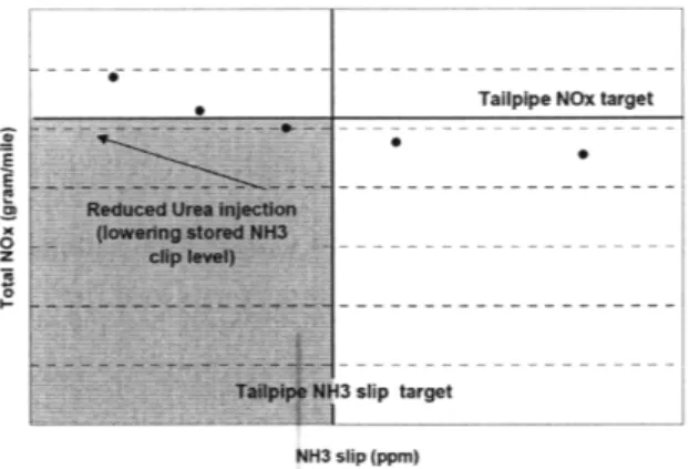
In a demonstration of model application for control purposes, the full scale catalyst was modeled as four individual segments with the urea injections determined by the amount of Stored NH3 in the second segment. As such, they were able to obtain a trade-off plot between NO, reduction performance and NH3 slip, as shown in Figure

1-5.

Species ent

E

Ta 1p H3 slip target

NH3 slip (ppm)

Figure 1-5: _{TradeOff plot between NO, and NH3}

Modeling for Control -State Space Approach

In the ASME article by Devesh Upadhys y and Michiel Van Nieuwstadt [8], the authors presented a lumped parameter state space model for the Urea SCR system. In the control oriented model, three states w re represented, namely the concentration of

NO (CNoX), concentration of NH3 (CvH3) and the surface coverage fraction of the

catalyst (0). While having similar conservation of energy and mass equations as Jeong Kim et. al., the model was of zero order and neglected the distribution gradient along the x-axis. Setting the boundary conditions as inputs, and using Orthogonal Collocation with the collocations points at the catalyst inlet and outlet, the state space model was presented as such:

Co, -&CNO, (OscRredO + ) + Roxesc 0

-= -(RadCNH 3 + Rdes + RredCNO Rox) + RadCNH3 0 U 0 d

NH NH 3 scRad

) +

with nomenclature as such:

C Concentration of each Species

0 Surface Coverage Fraction of NH3

O8s Total NH3 Storage Capacity of Catalyst Coating

R Reaction rates

F Exhaust Flowrate

V Catalyst Volume

U Gaseous NH3 injected

d NOx input disturbance

Y Measured Output

Using experimental results to verify the model predictions, the authors concluded that the lumped parameter model was sufficient in capturing the chemical performance of the catalyst, and that it should provide an adequate framework for control design.

Modeling for Control - Systems Identification Approach

In their SAE article, John Chi and Herbert DaCosta [6] presented their work on mod-eling and control of a Urea SCR system. While their starting point was similar to that of Jeong and Devesh, they proposed a different method of controlling the urea injections. Using their catalyst test bed, they determined the Normalised Stoichio-metric Ratio (NSR) N ) required for different levels of NH3 slip at different test conditions. Figure 1-6 shows the relationship between NH3 slip and NO, Reduction Efficiency at different NSR levels.

1.2 0.96 0.72 z 0.48 0.24 0-200

NOx Conversion and NH3 Slip Trade-Off Curves at 50,000 1/hr

Catalyst Space Velocity

-A NSR for 5 ppm NH3 Slip

-1 NSR for 25 ppm NH3 Slip

- NSR for 50 ppm NH3 Slip

-!-Conv for 5 ppm NH3 Slip

-B--Conv for 25 ppm NH3 Slip -- Conv for 50 ppm NH3 Slip

100 80 60-40 40 T 20 z 250 300 350 400 450

Catalyst Bed Temperature, degrees Celsius

Figure 1-6: NH3 Slip and NO, Reduction Efficiency against NSR

A control algorithm was developed using the map of NH3 Slip against NO, Reduction Efficiency for a range of operating conditions. With the temperature, space velocity, target NH3 slip level as inputs, the algorithm is thus able to estimate the achievable

NO, reduction efficieny, and the corresponding NSR for the injection. Subsequently, the response of the system to the range of NSR were captured and plotted in Figure

1-7 below.

Urea SCR System Step Response for different Urea Injection Levels @ 204 degrees Celsius and 7227 1/hr

1000 --- --- r r 1.25 900 800 - - - 1 700 - - - "-I0 600 -- ---- -- ---- 0.75 c 500 S400 - -- - - - - - 0.5 300 z 200 - - - - 0.25 100 0 0 0 50 100 150 200 250 300 Time, seconds

Figure 1-7: NO, Response to Urea

The authors proposed that the behavior of the NO, reduction can be modeled as a first-order system of the form shown below.

y(s) b a

u(s) s + ap (1.15)

con-ditions, namely inlet NO, concentraion, inlet NH3 concentration, amount of Stored NH3 on the catalyst coat, catalyst space velocity and exhaust gas temperature. This meant that both ap and bp would be mapped by a five-dimension look-up table. Us-ing the simplified first order transfer function, the authors then proposed to apply composite adaptive control with the following adaptive laws.

u = &,(t)r +

&,(t)y

ar = -sgn(bp,)er (1.17)

ay = -sgn(bp,)ey (1.18) where e is the error signal and 7 is the adaptation gain.

Chapter 2

Approach

Results from the literature search yielded many approaches to tackling the problem of controlling a Urea SCR system. While all of them began with a full chemistry model of the catalyst, the simplification of the full chemistry model into a form more suitable for applying control algorithms were varied. In this thesis, we take an alternate approach where input-output data, together with a system-identification procedure is used to determine low-order models of the SCR. In particular, a first-order model is derived, whose accuracy is then compared using a full-chemistry model, using NH3,in as the input and Stored NH3 as the output.

2.1

FTP Cycle

In order to understand the conditions under which to map the variables of the first order transfer model, the FTP-75 cycle was picked to be the benchmark [11] for vehicle operating conditions. The FTP-75 cycle is used for emission certification of diesel vehicles effective year 2000. It simulates different conditions of driving on the road, and consist of three phases: cold start phase, transient phase and hot start phase. Figure 2-1 shows the vehicle speed against time for the three phases[ll].

Cold stall phase 0-505 s iNi TIaisient phllase 505-1369 s

rlAitT

l

Inf

Hot stal phase

0-505 s

0 200 400 600 800 1000 1200 1400 1600 1800 2000

Tile. s

Figure 2-1: FTP-75 Cycle: Vehicle Speed against Time

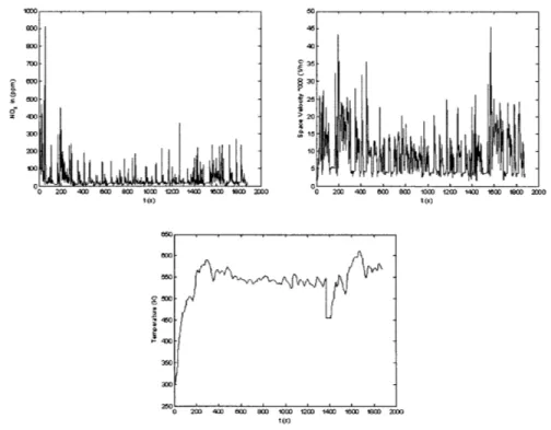
Translating the FTP-75 cycle vehicle speed and vehicle load into profiles for NO, in, Space Velocity and Temperature, we get a sense of the range of operating conditions that have to be mapped. Figure 2-2 shows the profiles for these catalyst inputs plotted against time. -o -0 o 9o o 2Wo 400 O 8s0 lO 120 1400 16 18oo00 OO t )

Figure 2-2: Input profiles for NOT, Space Velocity and Temperature

2.2

Diesel Engine Operating Conditions

Based on the FTP-75 Cycle input profiles, the trim points for mapping the first order transfer function were selected to be as follows:

NO, in (ppm) 87.5, 175, 262.5, 350

Space Velocity (1/hr) 10k, 30k, 45k

Temperature (K) 500, 550, 600

The number of trim points and spread between trim points were choosen based on a trial and error basis. Sufficient data points were selected such that the behavior of the state could be captured to an acceptable degree of accuracy, while minimizing the effort spent on capturing and calibrating the data points. A linear interpolation algorithm was used for all intermediate points.

2.3

_{First Order Linear Model for NH}

_Storage

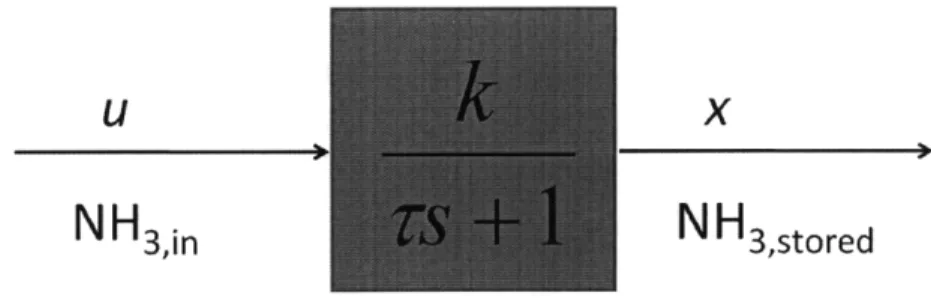
Using input-output data from the full chemistry model in [7], with NH3,i, as the input and Stored NH3 as the output, a a transfer function model was developed. This was of the form:

1 k

i = -- z + -u (2.1)

T T

where u denotes NH3,i, and x denotes Stored NH3. This model is shown in a transfer

U X

NH3,in

_NH

Figure 2-3: Block Diagram for Transfer Function Model where k and 7 are mapped by a 3-D or 4-D lookup table.

There are many ways to obtain the maps of k and 7 and the following methods were tested to determine the best approach.

2.3.1

Method 1: Bode Plots

Different input profiles of NH3 were introduced into the simulation, at different con-ditions as listed above. The input consists of both a step and sinusoidal wave. The sinusoidal frequency was changed over a suitable range determined by trial and error. The inputs were varied according to the following:

u = ao + aisin(2 ft) (2.2) where

a₀o 75 - 100% of NOx,in al 25 - 50% of NOx,in

f Frequency range from 5 x 10- 5 - 1 x 10-2 Hz

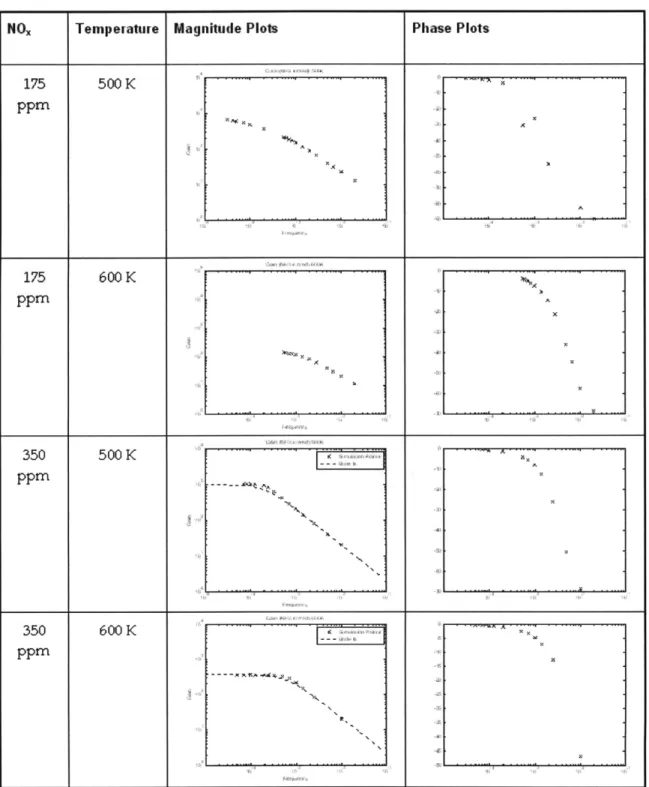
For each trim point, the frequency was varied in order to estimate the values of k and 7 through the unit gain and phase difference. Figure 2-4 below shows a summary of bode plots obtained for some of the trim points.

NOx Temperature Magnitude Plots Phase Plots 175 500K K Ppm 175 600 K ppm 350 600 K -ppm _{. . . . . . . ., . . . .} ,r r i ?:::: c., . : . . . ... . .. . . .

Figure 2-4: Bode Plot for determination of model paramters

By checking the the corner frequency and the DC gain of the magnitude and phase plots, the values of k and T could be estimated. However, this was not easily done for all the plots. As seen in Figure 2-4, some of the behavior observed did not produce bode plots that were expected of a first order function. A quick verification of the

k and 7 values that were obtained also showed that the numbers did not reflect an

accurate estimate of the state of NH3 storage. As such, an alternate method was needed to map the k and 7 values.

2.3.2

Method 2: Step Input

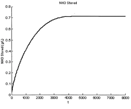
Using the full chemistry model in [7], a step input was applied to the system to trigger a response in NH3 storage. Using the final steady state value, and the rise time to 63% of the final steady state value, the values of k and 7 could be estimated. Figure 2-5 below shows a typical step response of the system.

NH3 Stored 0.8 0.7 0.6 : 0.5 -" 0.4 CO z 0.3 0.2 0.1 0 1000 2000 3000 4DU 5000 000 7000 800 t

Figure 2-5: Step Response of NH3 Storage to NH3,in

However, depending on the initial condition of the NH3 Storage, the k and -F values varied, and could not be adequately captured by a single value. A fourth dimension needed to be added to the map: NH3 Storage level. Also, the amount of NH3,i,

injected also affected the gain and time delay constants, due to the chemical nature of the system. As higher concentrations of NH₃,in were introducted, the system becomes less responsive to the injections and the gain values decrease. As such, two more dimensions were introduced to the mapping of k and 7.

NO, in (ppm) 0, 87.5, 175, 262.5, 350

Space Velocity (1/hr) 10k, 30k, 45k

Temperature (K) 500, 550, 600

Excess NH3,in (ppm) 0, 87.5, 175, 262.5, 350

NH3 Storage Level (g/L) 0, 0.01, 0.02, ... , 0.99, 1.00

Figure 2-6 shows the system responses to the same input with different initial condi-tions, and Figure 2-7 shows the system responses when overlapped.

NH3 Stored 1.4 1.2 0.8 0.4 0.2 0 1000 2000 3000 4000 5000 CO 70M0 8O

Figure 2-6: Family of System Responses with different Inital Conditions

As such, in order to capture the system response througout the whole range of NH3 storage, only two simulation runs needed to be conducted; one from zero initial stor-age, and one from about 30% initial storage. Using the two system responses, the NH3 Storage Level is broken down into steps of 0.01, and the values of k and T esti-mated for each step. Figure 2-8 shows the system response broken down into a family of step responses with incremental initial conditions.

NH3 Stored 1.4 1.2 1 fT 0.8 E m 0.8 0.4 0.2 0 1000 2000 3000 40 500 6000 7000 8000 9 0

Figure 2-7: Family of System Responses when Overlapped NH3 Stored 0.8 0.7 0.8 20.5 8 0.4 z 0.3 1002 2000 3000 4000 t 5000 8000 7030 8000

Figure 2-8: Single Step Response used Initial Conditions

to estimate k and T values for different of

To evaluate the accuracy of the k and 7 values obtained, the output of the transfer function model was compared to that of the full chemistry on a few sets of simulations. Within the boundaries of the mapping dimensions, the transfer function model was able to capture the NH₃ Storage behavior to a very good degree of accuracy.

2.3.3

Method 3: Small Step Disturbance

Instead of expressing the state of Stored NH3 as x, it can also be broken down into the following form:

X= - Xnominal + A

(

S 3 I I I I

where xnominal is the equilibrium value of Stored NH3, and Ax is the deviation from the equilibrium. The transfer function model can then be applied to the deviation

from equilibrium as such:

(s) =

(2.4)

u Ts +

The values of k and 7 can be determined from small perturbations from the equilib-rium value. While an additional map for Xnoinal needs to be obtained, it reduces the number of dimensions on the maps for the k and 7 values. Figure 2-9 shows a simulation run where the system was allowed to reach equilibrium, and small step perturbations of +/- 5 ppm of NH3,in were introduced. Similarly, the k and 7 values in this case could be estimated by the D.C. gain and the 63% percent rise time.

NH3 Stored 0.66 0.64 0.62 t 0.6 0.58 z 0.56 0.54 0.2 t x104

Figure 2-9: Small Step Perturbations

Using the Full Chemistry Model to map the values of Xnominal, k and 7 with small

step perturbations, this format proved to be the easiest to implement and calibrate. The maps obtained were saved using Microsoft Excel and imported by Matlab into a Simulink environment model. Model verification and subsequent control algorithm implementation were developed using this Simulink model as a base. A table of the

2.4

NH

Slip

as

a Function of NH

Storage

In order to complete the transfer function model for the Urea SCR system, two more states needed to be captured. These were the NH3 Slip and the NO, Slip of the system. Based on information obtained from the literature search, it was known that the adsorption of NH3,in by the catalyst surface coating was highly efficient. Expressed in equation form

Rad = kade RT (2.5)

where the activation energy in the equation (Ead) was set to zero in some full chemistry models. As such, it was logical to assume that any of the NH3,i, injected will be adsorped by the catalyst surface coating, and the NH3 Slip was a result of desorption

-Edes(1--"e )

Rdes = Kdese RT (2.6)

which was dependent on the surface coverage fraction of the system (0). As the surface coverage fraction is related to the state of Stored NH3 in the transfer funciton model, it was proposed that the state of NH3 Slip (yi) could be obtained as a function

of Stored NH₃ (x).

Yi = f(x) (2.7)

Using the Full Chemistry SCR model, simulation runs were designed such that NH3 Slip due to desorption was isolated and captured for the operating range as presented in the mapping stages. The Urea SCR System was first allowed to saturate with Stored NH3 until a suitably high equilibrium level was reached. The flowrate of the simulation was then sustained, but with NH₃,i, reduced to zero. The Stored NH₃ was noted to drop to zero gradually, while the amount of NH3 Slip per second was monitored and captured. Figure 2-10 shows a typical plot of the simulation run.

NH3 Stored 1.4 1.2 0.8 0.0 0.4 0.2 0 0 0.5 1 1.5 2 2.5 3 3.5 4 t x 10'

Figure 2-10: NH3 Slip due to Catalyst Desorption

Using the data captured for Stored NH₃ and NH3 Slip, the amount of NH3 Slip at each level of NH3 Storage could be matched and plotted. Figure 2-11 show the plot for one of the operating conditions, where Temperature, T = 600 (K), and Space Velocity, uin = 45,000 (1/hr).

NH Slip Against NH Stored

am

0 0.1 0.2 03 04 05 0.6 01 0. . 1

NH₃ Stored (gIL)

Figure 2-11: Plot of NH₃ Slip against Stored NH3

Repeating the NH3 Slip simulation runs across the range of mapping conditions, NH3 Slip could be mapped entirely as a function of Stored NH3, as as shown in Eq. (2.7). The complete map is included in a table format in Appendix D.

2.5

NO, Slip as a Function of NH

Storage

Similar the the mapping of NH3 Slip, the NO, slip can be derived from the efficiency level of the Urea SCR System, as a function of the level of Stored NH3.

Y2 = g(x) (2.8)

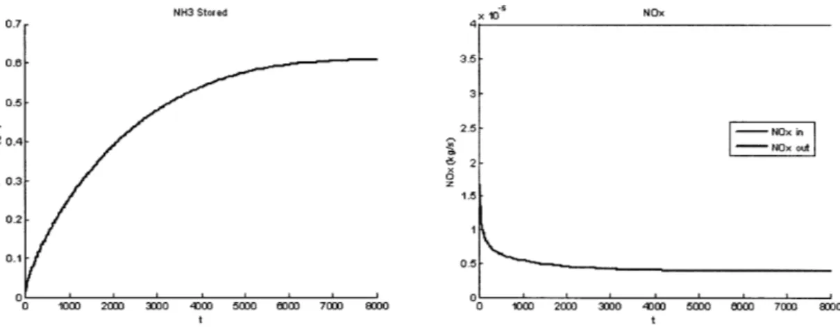
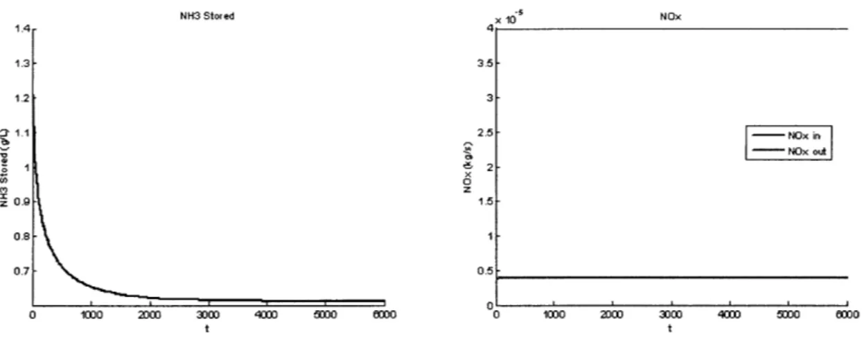
Using the Full Chemistry SCR model, simulation runs were designed such that NOx Slip for different levels of NH₃ Storage were captured. In order to capture the full range of data, two initial levels of Stored NH3 were used; 0 (g/L) and 1.4 (g/L). Starting from zero NH₃ Storage, the Urea SCR System NH3 Storage Level was slowly built up, while a constant flow of NOx,ij was introduced. The amount of NO, Slip, together with the amount of Stored NH3 were measured at each instant throughout the experiment. In order to determine the data for storage levels above equilibrium, the setup was repeated for a initial level of NH₃ Storage that was higher than equilibrium. Figures 2-12 and 2-13 shows a typical plot of Stored NH3 and NO, Slip for the setup.

NH3 Stored x 10 NOx 0.7 4 0.06 3.5 3 0.5 25 - NOx ouin 2-S0.3 1.5 0.2-0.1 0.5 0 1000 200 3000 4 00 SWo 000 7000 0000 0 1000 200 30 40 0 0 5000 0000 700O 8300 t t

NH3 Stored 1.4 1.3 1.2 1.1 , z 0.9 0.8 0.7 0 1000 2000 3000 4 t 10C 5000 3000 x10 NOx 3.5 3 2.5- - NOx in 2.5 NOx out 2 1.5-0.5 0 0 1030 2000 302 400 5000 50

Figure 2-13: Plots for Stored NH3 and NO, Slip with 1.4 (g/L) Initial Condition

The setups were repeated for the operating range presented above. Using the data captured for Stored NH3 and NO, Slip, the amount of NO, Slip at each level of NH3 Storage could be matched and plotted. Expressed as a percentage of NO,i, the NO, Slip fraction is plotted on the y-axis against the Stored NH3 on the x-axis. Figure 2-14 show the plot for one of the operating conditions; T = 600 (K), uin = 45,000 (1/hr).

NOx Slip against NH₃ Stored

09 05 0 0A0 Z 0.3-02 NH₃ Stored (g/L)

Figure 2-14: Plot of NO, Slip Fraction against NH3 Stored

Through examination of the simulation results, it was observed that the NO, Slip fraction was the same for varying values of excess NHa,in. Only when insufficient NHa,in were injected did the NO3 Slip fraction have a different value. In the Figure 2-14 above, the line with the poorer performance (shown in pink) was when insufficient NH3,in was injected, while the line shown in blue was when excess NH3,i, was injected.

Repeating the NO, Slip simulation runs across the range of mapping conditions, the NO, Slip fraction could be mapped entirely as a function of NH3 Stored, as proposed by the Eq. (2.8). The complete map is included in a table format in Appendix E.

Chapter 3

Control Using NH

3

Storage

Feedback

With the transfer function model fully determined, the next step was to start imple-menting control algorithms on the system. This took place in several steps. Control algorithms were first tested on the linear transfer model to ensure that minimal per-formance standards were achieved. Subsequently, the full chemistry model was intro-duced as the plant, with the transfer function model acting as the plant model, and the control algorithms were tested again. Since the amount of NH3 Slip and NO, Slip were functions of Stored NH3, setting a reference value for Stored NH3 and having the system track the reference would give the best chance of minimizing both NH3 Slip and NO, Slip. Starting with a Proportional-Integral (PI) Controller on the NH3 Storage, the closed loop system was first tested on a NO,,in profile of random steps and length, and subsequently proceeded more complicated profiles with variations in Temperature and Space Velocity. Building on a working PI Controller, an Adaptive PI Controller was also developed, implemented and tested.

3.1

PI Control

From the linear model proposed in Section 2.3.3, the transfer function model, as given by Eq. (2.3) and Eq. (2.4) were

X =- Xnominal + AX

Ax k

U Ts + 1

(3.1) (3.2)

Rewriting the above equations in a simpler format, we have

X = Xnominal ₊ X x

k

Figure 3-1 belows illustrates the Block Diagram of the transfer function model with a PI Controller added.

NH_3in

NH3,stored

Figure 3-1: Block Diagram for Transfer Function Model with PI Control

Setting the reference signal for X to be Xnominal, it can be observed that the controller

needs to maintain value of x at zero. Using PI control on a linear transfer function model, this can be easily achieved via the selection of the proportional gain(K) and integral gain (Ki) values, with the controller signal as such

=- EK+ - x (3.5)

From Eq. (3.5) for the control input, the complete closed loop transfer function model for the system becomes

x = - u (3.6) Ts + 1 x +I Kp + ) (3.7) (TS+l 1)x -k (K,+ - x (3.8) TiX + = -kKi - kKx (3.9) T- + (l + kKp) + kKix = 0 (3.10) S+ k : + -K 0 (3.11) T T

For a second order system, the differential equation can be expressed in the form

& + 2(wo: + wx = 0 (3.12)

where ( and wo are the damping ratio and natural frequency respectively. By fixing the damping ratio desired for the closed loop system, we can express Ki in terms of

k, T, and Kp. l+kKp = - =1 (3.13) 2 kK' 2 /kK 1 + kK, T T (3.14) kK, (1+ kKp)2 Ki = 4k (3.16) 4kT

adjust the performace of the system through the selection of proportional gain (Kp). Using a random NOx,in profile as shown in Figure 3-2, the closed loop performance of the system with PI control was plotted for a range of values of Kp values, and compared to the open loop performance where only a 1:1 (NHa,in:NOx,in) injection was supplied.

0 200 400 00 800 1000 1200 1400 1600 1800

Time(s)

Figure 3-2: Random NOx,i Profile for PI Control

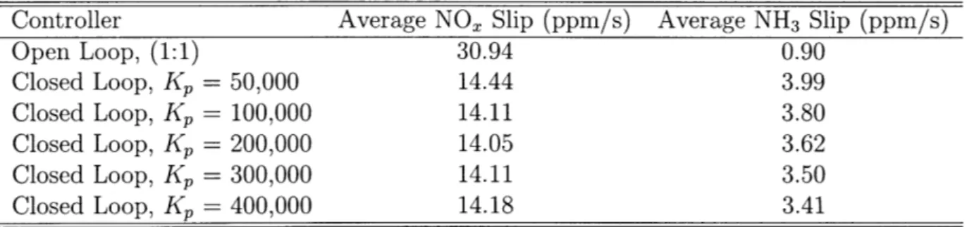
The following plots in Figure 3-3 show the results for a single set: Temperature: 500 (K), Space Velocity: 30k (1/hr), NOx,in Bound: 250 - 350 (ppm). The top left plot shows the amount of Stored NH3, the top right plot shows the amount of NOx Slip, the bottom left plot shows the NH3,i, and the bottom right plot shows the NH3 Slip. To translate the system performance into numbers, the total amount of NH3 Slip and

NOx Slip are summarized into a table format below.

Controller Average NOx Slip (ppm/s) Average NH₃ Slip (ppm/s)

Open Loop, (1:1) 30.94 0.90 Closed Loop, Kp = 50,000 14.44 3.99 Closed Loop, Kp = 100,000 14.11 3.80 Closed Loop, Kp = 200,000 14.05 3.62 Closed Loop, Kp = 300,000 14.11 3.50 Closed Loop, Kp = 400,000 14.18 3.41

NH3 Stored (500K) 35 NOx Slip Open 36- Kp= 50,000 - Kp= 100,000 - Kp = 200,000 0.5 2.5 - Kp= 300,000 - Kp= 400,000 0.4 R 2 S0.3 1.5 Open 0.2 Kp= 50,000 1 - Kp= 100,000 0.1I Kp= 200,000 0.5 Kp= 300;000 I Kp= 400,000 0 ; J 0 ' ' ' 0 200 400 600 800 1 1200 1400 1600 1800 2000 0 200 400 600 800 1000 1200 1400 1600 1900 2000 t t x104 NH3 in x 10 NH3 Slip 1.4 - Open - Open - Kp= 50,000 -~2 Kp= 50,000 - Kp= 100,000 1.2 - Kp= 100,000 - Kp= 200,000 - Kp= 200,000 - Kp= 300,000 1 - Kp= 300,000 - Kp = 400,000 Kp= 400,000 0.4 0.2 08 0 200 400 600 800 1000 1200 1400 1600 1800 2000 0 200 400 600 800 1000 1200 1400 1600 1800 2000 t t

For the range of operating conditions, the testing conditions were varied as follows: Set Temperature (K) Space Velocity (1/hr) NOx,in Bound (ppm)

1 500 30k 250 -350 2 500 30k 200- 300 3 500 30k 150 - 250 4 550 30k 250 - 350 5 550 30k 200 - 300 6 550 30k 150- 250 7 500 15k 250 - 350 8 500 15k 200- 300 9 500 15k 150 - 250

Table 3.2: Input Conditions for Sets 1 - 9

The tabular summary for performance of PI Control for Sets 1 - 9 are included in Appendix F.

3.2

Adaptive PI Control

With a working PI Controller, an Adaptive PI Controller algorithm could then be the next step in the testing sequence. Figure 3-4 shows the block diagram for the design adopted for Adaptive PI.

471~e

_X

-001

Figure 3-4: Block Diagram for Adaptive PI Control Design

form of the Adaptive PI Controller can be expressed as follows: Tnominal = Jel(t) + Bx + Ke 2(t) (3.17) where e = Xd- = --X (3.18) el -= Ae (3.19) e2= e +A e dt (3.20)

where the parameters of the Adaptive PI Controller (J, B, K, A) are to be determined. In the adaptive form of the control input, we apply the following adaptive laws:

7 = Jei(t) + Bx + Ke 2(t) (3.21)

J = 'le 2el (3.22)

B = yle2x (3.23)

where yl and '2 are the adaptive gains to be selected. The overall differential equation for the plant and adaptive controller becomes:

(

= -x - Bx + Jel(t) + Ke ₂(t)) (3.24)

and the error equation becomes:

e2 2(t) ( -

B)

Selecting the adaptive controller parameters such that the initial values matches of the PI controller, the performance of the adaptive controller can be evaluated against that of the PI controller. Table 3.3 list the initial values chosen for the adaptive parameters, and Figure 3-5 shows the comparison plot between the adaptive controller

and a PI controller for the same input conditions. A summary of the average NH3 Slip and NOx Slip is included in Table 3.4.

Adaptive Controller Parameter Value

Jinitial 10,000 Binitial 500 K 200 A 1 Y1 1000 'Y2 1000

Table 3.3: Adaptive PI Controller Parameters

Controller Open Loop, (1:1) Closed Loop, Kp = 50,000 Closed Loop, Kp = 100,000 Closed Loop, Kp = 200,000 Closed Loop, Kp = 300,000 Closed Loop, Kp = 400,000 Adaptive PI

Average NO, Slip (ppm/s) Average NH3 Slip (ppm/s)

30.94 0.90 14.44 3.99 14.11 3.80 14.05 3.62 14.11 3.50 14.18 3.41 14.18 3.39

Table 3.4: Set 1 Performance Summary including Adaptive PI Control

While the PI controller relied on the transfer function mapping of k and T values to determine the optimal gain for Ki, as observed by Eq. (3.16), it can be observed that the Adaptive PI controller relied only on feedback information and was able to achieve a comparable, if not better performance for the same input conditions. Further comparison of the performance between the Adaptive PI controller and the PI controller under different input conditions can be found in Appendix G.

NH3 Stored - Adaptive - Kp= 400, 000 - Adaptive Kp= 400,000 O. 1 1 1' 0 200 400 600 800 1000 1200 1400 1600 1800 2000 0 200 400 600 800 1000 1200 1400 1600 1800 2000 NH3 Injected x 1O4 4 .5r 4 3.5 3 2.5 1.5 0.5 Adaptive - Kp= 400,000 2 1.5 z x 108 3r NH3 Slip -Adaptive Kp= 400,000 U U 0 200 400 600 800 1000 1200 1400 1600 1800 2000 U 200 400 600 800 1000 1200 1400 1600 1800 2000 t t

Figure 3-5: Comparison Plots between Adaptive PI Control and PI Control

49 0.4 0.3 x 16 NOx Slip

i~

_-~--$

Chapter 4

Control Using NH

3

and NO, Slip

Feedback

Implementing feedback control using the state of Stored NH3 was applicable to the transfer function model as the NH3 Storage was one of the states of the model. On a actual vehicular Urea SCR System, the amount of Stored NH3 on the catalyst at any point of time will be unmeasurable, and thus will not availble for negative feedback. As such, a new feedback control algorithm that used the states that are available was required. Through the discussions with the research team at Ford Motor Company, it was understood that the current gas sensor that installed on the vehicular system gave a combined measurement of NH3 Slip and NO, Slip. The subsequent step was to implement PI and Adaptive PI Control using the combined state of NH3 Slip and NO, Slip.

4.1

PI Control

From the maps of NH3 Slip and NO. Slip presented in Eq. (2.7) and Eq. (2.8), we can present the combined state (z) as follows:

z = kif (x) + k2g()

where k and k2 were constant gains dependent on sensor behavior. The differential equations for z could be expressed as:

z(t) = a z(t) + bu(t) (4.3)

,, ( sf 6 g

a = ki 6 + k2 ap (4.4)

,

(

b = kif +k2 bp (4.5)

With the differential equation shown in the form as presented in Eq. (4.3), a fixed PI controller of the following form was proposed:

u = bz

+

= -(K+A)z-KAf zdt (4.7)

The plant, together with the proposed PI controller, will have the form:

zl = -kzl (4.8)

zi = z + A z dt (4.9) which predicts that the controller should drive to state z to zero, even if ap and bp are time varying. Using the mean values of k and 7 and the maps of f(x) and g(x) to obtain an estimate for ap and bp, the fixed PI controller was implemented on a full chemistry system to evaluate its performance and its ability to minimize both NH3 Slip and NOx Slip. Setting the z,,,omi,, at 90%, the following plots in Figure 4-1 present the results for the operating conditions of Set 1. Table 4.1 summarizes the average NH3 Slip and NOx Slip.

NH3 Stored 200 400 600 800 1000 1200 1400 1600 1800 2000 t 0.25 0.2 0.15 co 0.1 0.05 0 6 5 4 63 z 2 1 -NH3 in -NH3 out 0 O..0' 0 200 400 600 800 1000 1200 1400 1600 1800 2000 0 200 400 600 800 1000 1200 1400 1600 1800 2000 t t

Figure 4-1: Performace Plots for PI Control using z, Znominal = 0.90

2 NOx in 2.5 NOx out S 2 1.5 0 0.5

Controller Average NO, Slip (ppm/s) Average NH3 Slip (ppm/s)

Closed Loop 33.2 0.65

Table 4.1: Performance Summary for PI Control using z, Znominal = 0.90

From the numbers in Table 4.1, the controller seems to be able to track the efficiency

set (Znominal) of 90% pretty well. A repeat set with znoinal set at 95% was ran with

the following results. Figure 4-2 presents the plots for Stored NH3, NH3 Slip and NO, Slip. Table 4.2 summarizes the average NH3 Slip and NO. Slip.

Controller _{Average NO, Slip (ppm/s) Average NH3 Slip (ppm/s)}

Closed Loop 14.5 1321

Table 4.2: Performance Summary for PI Control using z, Znominal = 0.95

From the plots and the table summary, it can be observed that the PI controller was unable to avoid the positive feedback mechanism inherent in the Urea SCR System. With increasing values of z, the controller increased the injections of NH3, which furhter increased the values of z, thus resulting in a positive feedback. An Adaptive PI Controller was required in order to skirt this critical issue.

NH3 Stored 1.4 1.2 0.6 0.4 -02 0 200 400 600 800 1000 1200 1400 1600 1800 2000 t x 10 NOx x 104 NH3 S6- 1.2 4 - 0.8 S- NOx o ut ; 3- 0.6 SNH -NH 2 - 0.4 -1H 0.2 z z 0 200 400 600 800 1000 1200 1400 1600 1800 2000 0 200 400 600 800 1000 1200 1400 1600 1 t t

Figure 4-2: Performace Plots for PI Control using z, Znominal = 0.95

800 2000 3 i

4.2

Adaptive PI Control

For the differential equation of z in Eq. (4.3), an Adaptive PI Controller of the following format is proposed:

u = 0 (t)z + 0o(t)zo (4.10)

= -(K + A)z-KA zdt (4.11)

zl = z

+

Oz = -bp(t)zlz (4.13)

9o = -bp(t)zlzo (4.14)

Implementing the Adaptive PI Controller on the same set of operating conditions as before, with znominal set at 90% and 95%, the plots in Figures 4-3 and 4-4 show the output for NH3 Slip and NO, Slip. The numerical results are summarized in Tables 4.3 and 4.4.

Controller _{Average NO, Slip (ppm/s) Average NH3 Slip (ppm/s)}

Closed Loop 31.7 0.70

Table 4.3: Performance Summary for Adaptive PI Control using z, Znominal = 0.90

Controller _{Average NO, Slip (ppm/s) Average NH3} Slip (ppm/s)

Closed Loop 16.4 8.20

Table 4.4: Performance Summary for PI Control using z, znominal = 0.95

From the plots in Figure 4-4, it can be observed that the Adaptive PI Controller does successfully avoid the positive feedback that occurred in the PI Controller. However,

0.25 0.2 0.15 0.1 0.05 NH3 Stored 0 200 400 600 800 1000 1200 1400 1600 1800 2000 t NOx x 10 -6r -NOx outn -NOx out x 105 6r 0 200 400 600 800 1000 1200 1400 1600 1800 2000 0 200 400 600 800 1000 1200 1400 1600 1800 2000 t t

Figure 4-3: Performace Plots for Adaptive PI Control using z, Znominal = 0.90 -NH3 in

KjliJJ ~ NH3 Stored 0 200 400 600 800 1000 1200 1400 1600 1800 2000 t x 1o0 NOx 6 4 -NOx in -NOx out x 10 7 r 3- 2- 1-0 200 400 600 800 1000 1200 1400 1600 1800 2000 0 200 400 600 800 1000 1200 1400 1600 1800 2000 t t

Figure 4-4: Performace Plots for Adaptive PI Control using z, Znominal = 0.95

- NH3 in -NH3 out