Active control of supersonic impingement tones using microjets

Active Control of Supersonic Impingement Tones

using Microjets

by

Jae Jeen Choi

Submitted to the Department of Mechanical Engineering

in partial fulfillment of the requirements for the degree of

Master of Science in Mechanical Engineering

at the

MASSACHUSETTS INSTITUTE OF TECHNOLOGY

September 2003

@

Massachusetts Institute of Technology 2003. All rights reserved.

A uthor ...

...

Department of Mechanical Engineering

August 8, 2003

Certified by...

...

- - . ... ... ...

Anuradha M. Annaswamy

Senior Research Scientist

Thesis Supervisor

A ccepted by ...

...

Ain A. Sonin

Chairman, Department Committee on Graduate Students

MASSACHUSETTS _INSTITUTE OF TECHNOLOGY

Active Control of Supersonic Impingement Tones using

Microjets

by

Jae Jeen Choi

Submitted to the Department of Mechanical Engineering on August 8, 2003, in partial fulfillment of the

requirements for the degree of

Master of Science in Mechanical Engineering

Abstract

High speed jet impinging on an obstacle generates distinct noise. If the jet flow exits with supersonic speed, the noise becomes more profound and causes many detrimental effects to the environment. STOVL exposed such tones experiences many adverse effects such as lift loss, sonic fatigue on the aircraft structure and ground erosion. Until now the impinging tone along with several adverse effects are thought to be originated by the feedback mechanism due to the presence of wall near the nozzle exit. As the acoustic waves reach the nozzle lip they excite the instability traveling downstream in the jet shear layer. These instability waves rapidly develop into large-scale coherent shear layer structures while traveling downstream. On impinging on the ground plane, this structure generates high amplitude pressure fluctuation, which generates acoustic wave, thus completing feedback loop. Hence, the noise reduction trial should be conducted to disrupt the feedback loop.

Many researchers have tried to destroy the feedback loop using passive and active way, but the reduction was confined only on specific operating conditions or so small extent compared to no control case. Recently, an attempt [1] using microjet showed a promising result. Because it is micro-scaled valve created by MEMS technology, microjet can be placed on any location without any space limitation and optimal flow control is possible by activating the supersonic microjet to desired command. In addition, since the microjet just affects the target properties without interfering other physical condition, it was accepted as the desired actuator. In this thesis, a special control strategy based on POD mode showed better reduction throughout several operating conditions. It is a kind of a parametric control strategy which sets the microjet pressure proportional to the shape of the most energetic mode. The reasoning for this control is based on the fact that the supersonic microjets attached near the nozzle exit may disrupt the feedback loop partially intercepting the upstream propagating acoustic disturbance or distort the coherent shear layer instabilities consequently disrupting their interaction with the acoustic field.

So far, the analysis based on a model has not been tried in depth. The second con-tribution of this thesis is the development of a reduced-order model. In this literature,

an updated form of Tam's [40] describing impinging jet on a wall, is suggested and its validity is supported from several experimental data conducted in Florida State Uni-versity. Furthermore, the mechanism of noise reduction and the effectiveness of the POD based closed-loop control strategy is introduced. Finally, a closed-loop control strategy expecting uniform reduction regardless of the ground effect over the entire range and varying operating conditions is experimentally tested and implemented in a STOVL facility at Mach 1.5.

Thesis Supervisor: Anuradha M. Annaswamy Title: Senior Research Scientist

Acknowledgments

First of all, I would like to thank Professor Anuradha M. Annaswamy for her nice guidance for the past 2 years. During those days, her advice gave me good intuition and a way of thinking needed for solving many engineering problems. I owed a lot of things to my research group members. I think the group is ideal combination in that each one has great talent that the others do not have. Prof. Ghoniem, a great scholar in Fluid mechanics area, brought confidence in making the impingement tone model. Dae Hyun Wee is mathematically well trained, Sung Bae Park has great intuition on solving engineering problems. I thank all of them for keeping an eye on my research and giving a constant feedback. I also owe a great deal to my colleague Sahoo not only for research work but for improving my language skill. Whenever I confronted a problem, discussions with him always give me a breakthrough.

I appreciate to Florida State University members too much, especially Prof.

Krotha-palli, Prof. Farrukh Alvi and his students, Okechukwu Egungwu, Huadong Lou. Because they are the experimental experts, we can do our research more efficiently. Without their efforts, I couldn't complete the experiment yet. Working with them was great pleasure to me.

I specially thank to my parents. Byung Tae Choi and Jung Mi Park. They

initiated my dream studying in MIT and encouraged me to make it come true. Finally,

I appreciate to my brother, Jae Woong Choi, for helping me to be mentally strong

during life in U.S.

This work was supported by a grant from the Airforce Office of Scientific Research, through the Unsteady Aerodynamics and Hypersonic program.

Contents

1 Introduction 10

2 Reduced Order Model of Impingement Tone

2.1 Physical Model and Its State-Space Form ...

2.1.1 Vortex Sheet Model . . . . 2.1.2 A Control-Oriented Model . . . . 2.1.3 Model Validation . . . . 2.1.4 State-Space Equations . . . . 2.2 Proper Orthogonal Decomposition . . . . 2.2.1 The Karhunen-Loeve Expansion . . . . 2.2.2 Optimality of the Karhunen-Loeve Expansion . . .

2.2.3 Method of Snapshots . . . .

3 POD-based Closed-loop Control Strategy

3.1 The POD method in flow field . . . ..

3.2 The Control Strategy . . . .

3.3 The Experimental Support . . . .

3.3.1 The Experimental Setup . . . .

3.3.2 The Previous Study . . . .

3.3.3 Result and Possible Mechanism of Microjet Effect

4 Summary and Concluding Remark A Tables 15 16 16 25 26 28 30 31 32 35 39 40 41 44 44 48 50 54 56

List of Figures

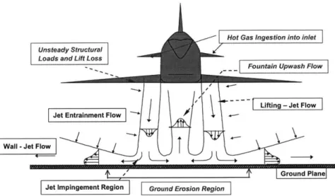
B-1 Flow field created by the propulsion system around a STOVL aircraft 59

B-2 Instantaneous shadowgraphs of a supersonic impinging jet at NPR =

3.7, h/d = 5.5 . . . . 59

B-3 The experimental set up of Fluid Mechanics Research Laboratory in Florida State University . . . . 60

B-4 Schematic of the experimental arrangement . . . . 60

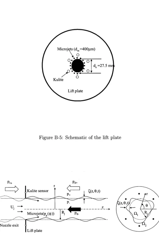
B-5 Schematic of the lift plate . . . . 61

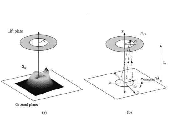
B-6 Vortex-sheet model for impingement tones control problem . . . . 61

B-7 Expected shear layer intensity distribution (a), coordinate system used for calculating acoustic excitation (b). . . . . 62

B-8 Schematic diagram of PIV mearsuring process . . . . 62

B-9 Instantaneous shadowgraph images of a supersonic impinging jets with-out (a) and with control (b) at NPR = 3.7, h/d = 4 . . . . 63

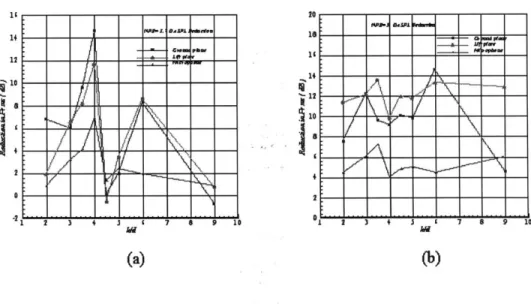
B-10 Reductions in fluctuating pressure intensities as a function of h/d, NPR = 5 (a) and NPR = 3.7 (b) . . . . 63

B-11 PLS images taken at one diameter downstream of nozzle, NPR = 5.0, h/d = 4.0; (a)Instantaneous image, (b)Time-averaged image . . . . . 64

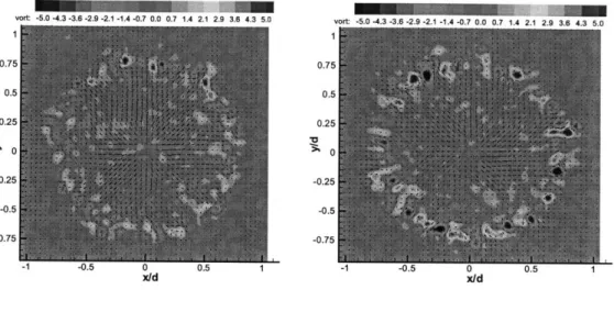
B-12 Streamwise vorticity distribution at the z/d = 1.0 cross plane of the jet flow NPR = 5.0, h/d = 4.0; (a)Instantaneous image, (b)Time-averaged im age . . . . 65

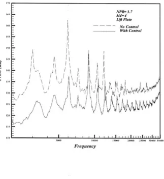
B-13 Frequency spectra for unsteady pressure on the lift plate of NPR = 3.7, h/d = 4.0 . . . . 66

B-14 Microjet effectiveness on different trials (NPR = 3.7) conducted on

Sep. 2000 (a) and Dec. 2001 (b) . . . . 66

B-15 Frequency spectra for unsteady pressure on the lift plate of NPR =

3.7, h/d = 6.0 (a) and model prediction of NPR = 6.0 (b) . . . . 67

B-16 The idealized centerline velocity . . . . 68 B-17 Frequency spectra of the unsteady pressure on the lift plate at NPR =

3.7: (a) Experimental data, and (b) Model prediction. Note that the

amplitude scales in (a) and (b) are different. . . . . 69

B-18 Variation of frequency of three impinging tones with h/d at NPR =

3.7: (a) Experimental data, and (b) Model Prediction. . . . . 70

B-19 Peak frequency interval of experimental data and model prediction

(

NPR= 3.7, M = 1.5 ) . . . . 71

B-20 The first mode shape and suggested pressure for each height. x axis is transducer position, y axis is normalized mode value . . . . 72

List of Tables

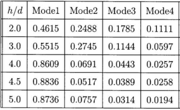
A.1 The energy content of the first four modes at each height (NPR=3.7) 56 A.2 Comparison of peak frequency interval (Hz) NPR=3.7, M =1.5 . . . 57

Chapter 1

Introduction

High-speed jet issuing from the nozzle often generates the acoustic field dominated

by discrete, high-amplitude tones. For example, screech tones are present in

non-ideally expanded jet, edge tones are dominant in the presence of edge shaped body and impingement tones are conspicuous when a supersonic jet impinges on a surface. Those tones are undesirable for any kind of mechanical system in itself because they cause a very detrimental effect such as sonic fatigue on the body facing the noise source. Especially, the impingement tone is unfavorable in designing efficient Short Take-off and Vertical Landing(STOVL) aircraft. Besides the purely acoustic damage, the flow field induced by the resonance brings very severe adverse effects on the ground and the aircraft itself too as described in Fig. B-1. The flow field causes the ambient flow to entrain into the gap between the aircraft and the ground that a large amount of lift loss are generated. The engine inlet suffers from hot gas ingestion and the ground erosion happens from impinging hot flow. These phenomena are thought to be more serious in the JSF(Joint Strike Fighter), a new version of STOVL aircraft, because the operating condition is supersonic [29] region. The understanding of the impinging jet flow is definitely necessary in designing the STOVL aircraft.

Hence, many researchers have tried to find the origin of noise sources and suppress them using various ways so far. Regardless of the specific nature of the tones, a host of studies on the aeroacoustics of impinging jets by Neuwarth [24], Powell

[281,

Tam and Ahuja [40], and more recently Krothapalli et al. [19] have clearly established

that the self-sustained, highly unsteady behavior of the jet and the resulting imping-ing tones are governed by a feedback mechanism. It is well-accepted that they are governed by a feedback mechanism that strongly couples the fluid and acoustic field and this coupling occurs in the jet shear layer near the nozzle exit, a region of recep-tivity. These feedback interactions occur thus: Instability waves are generated by the acoustic excitation of shear layer near the nozzle exit, which then convect down and evolve into spatially coherent large-scale structures. On impinging on the ground, these structures generate high amplitude pressure perturbation, which in turn pro-duce waves of neutral acoustic mode of the jet. As the acoustic wave reaches to the nozzle exit, it excites the shear layer again, thereby closing the feedback loop.

The presence of such large-scale structures, not normally present in such high speed jets, can be confirmed from the shadowgraph image shown in Fig. B-2. The high entrainment rates of the ambient fluid associated with such large-scale structure are thought to be largely responsible for the increased lift loss.

The logical approach to controlling the adverse ground effect is to disrupt the feedback mechanism responsible for this behavior. A number of researchers have attempted various passive and active methods in order to accomplish this goal. In the context of intercepting the feedback loop, Glass [12] and Poldervaart et al. [26] tried a passive control method by placing a plate normal to the centerline. In this way, they were able to reduced the overall noise level a certain degree. Motivated

by the previous result, Elavarasan et al.[11] conducted similar experiment and have

achieved about 11 dB reduction in the overall sound pressure level and recovery of about 16% lift loss. This passive control method appears to weaken the feedback loop and prevent the onset of self-sustained oscillations in the jet and result in the suppression of large-scale motion. However, the effect of such a passive approach is confined to a limited range of operating condition, especially for impinging jets. Because a small change in distance between nozzle to ground plate (h/d) leads to significant change in amplitude and frequency of impinging tone (Alvi and Iyer [2]), the control strategy for the suppression of the impinging tones should be active and

suggested more recently, in the literature (for example, Sheplak and Spina [32], Shih et al. [33]). In Sheplak and Spina [32]), Sheplak and Spina used a high speed co-flow to keep the main flow jet from acoustic wave. Their investigations showed a reduction of 10-15 dB in the near field broad band noise under specific core to ambient velocity ratio. To realize the effect, it was required for the co-flow flux should at least be 20% to 25% of the main jet. Shih et al. [33], upgrading the experiment, used a counter co-axial flow near the nozzle exit and were able to suppress screech tones of ideally expanded jet. However, those active control schemes required additional design modification in the nozzle part and high operating power. Consequently, such approaches are somewhat impractical for implementation in a real aircraft.

A few years ago, a study was initiated at the Fluid Mechanics Research

Labo-ratory (FMRL) of Florida State University, in Tallahassee, Florida, with the aim of understanding and controlling supersonic impinging jet flows in order to substantially reduce the ground effect. In this study, Alvi et al. [1] and Shih et al. [35] used arrays of supersonic microjets to control supersonic impinging jets and successfully reduced lift loss by as much as 40% accompanied by a 10-11 dB reduction in the fluctuating pressure load on the lift and ground surface. They introduced microjets for noise reduction with the same motivation as the aforementioned papers trying to shield the main jet from outer acoustic perturbation but the result was more dramatic.

In Alvi et al.'s[1] paper, we can see the microjet effect on noise reduction was much greater than any other actuators so far. However, the performance using the microjet actuators was observed to depend too much on the height. It should be noted that the control strategy used was one where air-flow was introduced through the microjets at a constant 100 psi chamber pressure. This strategy is referred to as "symmetric control" in this thesis, and can be viewed as an "open-loop" control strategy which neglects changing flow conditions for different heights. Hence, to achieve a uniform performance for the different operating condition, a different control strategy that "adapts" to the changing flow conditions should be introduced. Such an active-adaptive strategy should take into consideration the changing flow conditions during taking off and hovering moment of the real STOVL aircraft.

The microjet has many advantages over previous actuators from manufacturing, designing as well as practical points of view [1]. For example, microjets can be produced in large quantities to lower the unit production cost. Because of the small size, they can be operated without any spacing limitation and consume a small amount of flow rate to cause the reduction effect. Along with other electrical devices, they can be integrated into sensor/actuator active control system. Moreover, in contrast to the traditional passive control method, each microjet can be switched on and off strategically that it will be able to avoid the degradation of performance when the control is not necessary.

In the previous paper [35], the fluctuating pressure reduction achieved by using constant microjet pressure intensity (100 psi) along the nozzle was too dependent on the height change. In the search for some parameters expecting even noise reduction, he found that there are several parameters affecting the performance of microjet ef-fectiveness such as microjet pressure, injection angle, the distance from lift plate to ground and nozzle pressure ratio (NPR) etc. These parameters do have an impact on the performance of the actuators and can be adjusted for the best effect under a specific nozzle condition. But the degree of effect achieved from optimally adjusted parameter is far below the desired amount and still works better only under a specific operating conditions (under-expanded case). In fact, we have another degree of free-dom which was not considered in his study which is the variation of microjet intensity along the azimuthal direction.

Motivated by the above idea, in [20], we tried the experiment adjusting pressure distribution along the nozzle exit using an unique control method called "mode-matched control." It was somewhat ad hoc control strategy without considering the mechanism governing the flow and impingement tones. Fortunately, the mode-matched control strategy brought a large amount of OASPL reduction compared to the passive control method, symmetric control, had achieved. It was a very promising result because the new control strategy always showed lager reduction at all different heights and caused great amount of reduction around 9 dB where the passive control can not make any change. This is the main contribution of this thesis.

In the chapter 2, an impingement tone model called "vortex sheet model" will be presented. To implement closed-loop control in real-time, a reduced-order model of this system is needed. The model based on a vortex-sheet is discussed in chapter 2. Chapter 2 also covers a short explanation about Proper Orthogonal Decomposi-tion(POD) method as a very useful way to capture the dominant dynamics from a model. The optimal property of POD and the practical way to implementing POD (method of snapshot) is then introduced at the end of chapter 2. In the chapter 3, the new control strategy called "mode-matched control" will be presented. The ex-perimental result using the strategy and the noise reduction mechanism by microjet will conclude the chapter. Summary and concluding remark are presented in chapter

Chapter 2

Reduced Order Model of

Impingement Tone

In order to design a closed-loop control strategy, we adopt a model-based approach. A model of impingement tones, however, is quite difficult to derive due to the changing boundary conditions, compressibility effects, and the feedback interactions between acoustics and the shear-layer dynamics present in the problem. Since our primary goal is to model the impingement tone dynamics and how they respond to microjet-control action at the nozzle, we will derive a reduced-order model that only captures these dominant dynamics and the effect of control. For this derivation, while tools based on stability theory [18] can be used to obtain some of the parameters such as the tonal frequencies, they are inadequate for deriving other model-details due to the complex features of the flow field. Instead, we use the Proper Orthogonal Decom-position(POD) method and key measurements in the flow field to derive the model. This model in turn is used to derive an appropriate closed-loop control strategy.

At the beginning, this chapter will present a vortex sheet model of impingement tone and its state-space form will be suggested. At the following section, the general theory about Proper Orthogonal Decomposition(POD), a method for data compress-ing, and its optimality will be suggested. The theory encompasses from the definition of Karhunen-Loeve expansion and its optimality to a method of snapshot :a practical method implementing POD method. It is the summary of the some articles written

by A.J. Newman [25], L. Sirovich [36],[37],[38] and G. Berkooz [7].

2.1

Physical Model and Its State-Space Form

Model identification is one of the major tasks for designing control system and the most difficult job. In this chapter, an effort was driven to find out a suitable model for impingement system based on the previous researchers' idea. The validity of the system will be testified thorough the capability of predicting the peak in frequency domain under varying operating conditions. Based on the model, the state-space equation for control implement will also be driven.

2.1.1

Vortex Sheet Model

To control a certain physical system, it is desired to identify the mechanism governing the system. With the help from model, we can find out suitable control law and output parameter which captures the system characteristics well. That is the reason many researchers made an effort to make a plausible model of the impingement tone in spite of the difficulties.

Even though it is very difficult work to model the supersonic impinging jet due to complex phenomena such as compressibility of media or interaction between flow and acoustics, many researchers have tried to seek the proper model which mimics the real system fairly well. Previous investigators such as Wagner [44], Neuwerth [24], Ho

& Nosseir [16], Umeda et al. [42] believed that the impingement tones are generated by a feedback loop. Provided energy from the instability waves in the mixing layer of

the jet, instability waves are generated from acoustic wave in the region of nozzle exit. These waves magnify themselves as they are swept down to the down stream. On impinging on the ground, the acoustic waves are caused by high pressure fluctuation of the grown large scale vortical structure. According to Wagner and Neuwerth [24] the acoustic waves propagate to upstream inside the jet column for subsonic impinging jets. On the contrary, Ho & Nossier [16] suggested the propagating waves travel solely outside the jet column. However, regardless of whether the waves go inside or outside

the jet, on reaching near the nozzle exit it excites the shear layer of main jet and completes the feedback loop of noise generation.

By the feedback condition between the flow instability and the upcoming acoustic

wave, the impingement frequency can be calculated from the time required for the feedback loop to complete its cycle. The impingement tone frequency fN is

deter-mined from the following formula proposed by Powell [27]:

N+p + (N 1, 2, 3,...) _(2.1)

f N Ci Ca

Here h is the distance between the wall and the nozzle exit and Ci and Ca are the convection velocities of the downstream-travelling large scale structures and the speed of upstream-travelling acoustic waves, respectively. N is an arbitrary integer and p represents a phase lag, which is caused by the phase difference between the acoustic wave and the convected disturbance at both the nozzle exit and the source of sound. Owing to the difficulty of measuring these velocities experimentally, especially in supersonic jets, most previous investigators assumed a constant value for Ci as the

60% of the main jet velocity, but it is not strictly the case. Especially at the different

height, the value changes from 50 % to 60 % of the main jet velocity.

Likewise Powell, Neuwerth suggested the following relation in his paper [24]. It starts from the idea that the total number of periods in the feedback loop must be an integer.

h = xAst = (n - x)A,

f

= ca/As = cst/Ast (2.2)

From the above equations, we can derive the following equation for the discrete frequency generated by the feedback:

h = distance between plate and nozzle aperture

n = total number of periods

X number of vortex periods

Ast

between plate and nozzle aperture

As= acoustic wavelength C = phase velocity of vortices

Ca = speed of sound outside jet

Similar to the role of N did in Powell's relation, an arbitrary integer

n

causes a staging phenomena, abrupt jump in dominant frequency as distance h changes. In the above feedback model, while the downstream instability waves is relatively well defined (Michalke [23]), the feedback acoustic wave are somewhat unclear. Wagner [44] attempted to make this wave as a plane wave. However this model was not concrete enough and some characteristics derived from the model did not support the experimental data well and moreover it couldn't predict the Strouhal number of the impingement tone with satisfactory accuracy. Ho & Nosseir's model [16] was too simple to contain any particular spatial mode structure or property either. More recently, Tam brought one model, a jet as a uniform stream bounded by a vortex sheet in his paper [40]. His trial was able to give the reason why the helical mode in large scale vortical structure was impossible for the subsonic jet flow but couldn't explain the staging phenomena at all.

In control's point of view, it is ideal to construct an exact model. But, practically, it is almost impossible to make it identical to physical system for its complexity and unexpected parameters. Hence, in this thesis, I suggest a simple model which can show one of essential characteristics, the staging phenomena because system's resonant frequency corresponding to the peak is very important in that this represents a pattern of its behavior. The objective of a plausible model of the impingement tone was to be focused on predicting the peak frequency for varying condition for the uncontrolled case and finding out the most effective and optimal control method for suppressing the noise for the controlled case.

given a clue for developing the more discreet model. The model suggested in this thesis is modified version of the Tam's trial made in his paper [40]. The basic dif-ference between Tam's model and experimental setup of Fluid Mechanics Research

Laboratory in Florida State University will be mentioned afterwards.

The reduced-order model adopted for the control of impingement tones is based on the vortex-sheet jet model of [40]. Within a short distance(0.01Rj) downstream from the nozzle exit, the jet can be idealized as a uniform stream of velocity U and radius Rj bounded by a vortex sheet. Small-amplitude disturbances are superimposed on the vortex sheet (see Fig. B-6). This neglects the effect of the shock structure due to the microjet action and due to underdeveloped jet (if any) and the boundary effect of the ground. Let pd+(r, 0, z, t) and pd- (r, 0, z, t) be the incoming pressure wave associated with the disturbances outside and inside the jet, denoted respectively

by domain Q1 and Q2 where Q1 denotes jet-core which extends from z = -oc to

z = +oo, Q2 denotes the domain outside the jet-core and (r, 0, z) are the cylindrical

coordinates. pr+(r, 0, z, t) is the pressure wave reflected from lift plate. This wave has equal magnitude but opposite direction to the incoming one. Also, let ((z, 0, t) be the radial displacement of the motion of a compressible flow, it can be shown that the governing equation and r-direction momentum equation for the problem are:

1 a

2

_Pd±

2 t2 = V2pd+ (r E Q2)

+_= V2Pd- (r E Q1 ) (2.4)

Especially at r = Rf and z = Znozzie,

av+ _ _{1 ap+}

at p ar

-+U

1

ap

(2.5)

at

aoz

Pj

ar

At r -- oo, p+ satisfies the bounded condition. Where ao and aj are the speed of

sound outside (Q2) and inside (Q1) the jet and Uj is the main jet speed.

Pd+(r, z, 0, t)

Pd_(r,z,, t) ((Z, 0, 0)

Pd+(r)

Pd- (r) ei(kz+nO-wt)

where n = 0, ± 1, ± 2,... and k, the wavenumber and w (w>0), the angular frequency

are as yet unspecified parameter. Substituting the solution (2.6) into (2.4), it leads to the following eigenvalue problem about Pd+ and id_:

d2Pd++ 1 dPd+ - 2Pd+ + W

dr

2 _{2 2P1+}

-r d-r r [ao d2Pd- 1 dPd_ n2 (w - Ujk)2 dr + -Pd- ₂ dr2 r dr r2 a3

The solutions of (2.7) and (2.8) give

k 2Pd+ = 0 k2kPd_ = 0 (2.7) (2.8) (2.9) (2.10) Pd+ = CiHn~1)(r+r) Pd- = C2Jn(r/ r)

where H,' is the n th order Hankel function of the first kind, JT, is n"t order Bessel function of the first kind, 7+ = P (w2_/a2

- k2)), r_ = [( - Ugk)2/aj - k2 and C1 and C2 are unknown constants which are to be determined from boundary conditions.

Tam, in his paper, mentioned the necessary boundary conditions that make the problem well-posed, are as follows.

* Dynamic condition r = Rj: (2.11) * Kinematic condition r = Rj: (2.6) P+ = P-V+ = V_

This is definitely a necessary requirement for his model. As seen in Fig. B-6, the impingement tone system of his paper is different from the experimental setup of Fluid Mechanics Research Laboratory in Florida State University in that Tam's model does not have a lift plate which makes the problem more complicated. In reality, the shear layer near the nozzle is usually excited from the acoustic wave generated from downstream mixing layer. In addition to these direct influences, it is excited by the bouncing acoustic wave from the lift plate near the nozzle exit too. These direct and reflected acoustic wave intensify the flow interaction with it and magnify the excitation of the shear layer more violently than simple nozzle without lift plate. Hence, the previous dynamic and kinematic equality condition are should be modified especially at near the nozzle exit as:

Condition 1 Dynamic condition r = Rj:

P+-P- = Ap6(z - )ei(nOwt) (2.12)

where p+ represents the outside pressure field, the superposition of the acoustic wave

(Pd+) travelling upstream, and a wave reflected from lift plate (pr+) propagating in the opposite direction with an equal magnitude, i.e., Pr+(r, 0, Z, t) = Pd+(r, 0, -z, t).

p_ represents the inner pressure field inside the main jet, and Ap denotes an imposed

pressure jump across the shear layer.

Condition 2 Kinematic condition r = Rj:

V+ - V_ = Av 6(z - E)ei(no-t) (2.13)

where v+ represents the outside radial velocity field, v- represents the inner radial velocity field and Av represents an imposed velocity jump across the shear layer.

Mathematically, the pressure field in the entire flow field can now be expressed as

follows.

P+ =Pd+ +PrI

= A1H(1)(r,+r)cos(kz)e(nO-wt) (2.14)

where constant A1 and A2 are to be obtained from boundary conditions.

The pressure and velocity jump Ap and Av are imposed due to the presence of the ground plane and can be determined as follows. We model the ground effect

by introducing 'virtual' acoustic sources on the ground plane. In particular, infinite

number of monopoles are assumed to be present at z = L, along a circular line of radius r =

Rj,

with strength S, varying along the azimuthal coordinate 0. The source strength is the influenced by the jet vortical structures impinging on the ground plane and is assumed as

S(0) = Kp+(r = Rj, 0, z = L) (2.16)

where K is a proportional constant whose value can be estimated by comparison with the experimental data (see Fig. B-7). Using equation. (2.16) and Fig. B-7, we then calculate Ap and Av from the sum of pressure excitation caused by each monopole:

Ap e4" 0 ) = i Apmonopole(O; 01)dO

a d S (0; n) a bmono ole dO (2.17)

and

Av

e"i(nAwt)

j

VmonopoledO

(2.18)

0r

where 01 is the azimuthal location of interest, Apmonopole(0; 01) is the pressure exci-tation at the collecting point (01) on the lift plate due to a monopole placed at 0

of the ground plane,

#monopole

is the velocity potential due to each monopole placed on ground plane, and p3 is the density of medium in the jet nozzle. The velocity

potential in a moving media can be expressed as[13]

exp -it - Mz X2 + 2 1 - M F c ( 1 - M ) 3 1 -= 2) . . (2.19) (1 - M2)0.5

(

2 +X 2 + Y2) 1 -M

where w is frequency of acoustic wave in radian, c is sound speed and M1 is the Mach

number of moving media. Therefore equation (2.17), (2.18) become

(iwM

1L i _

exp + 1 l(0;1)

Ap ei"l = 27r 27ripj

wS.(0;

n)

I

- M c( - M)U d

Jo l(O; 01) (1 -M2) 05.'

(2.20)

exp - + 2 ;10S

I

Av

e/2' 2irS.(O; n) t

~

O) 1 - My c (1 - 1F)dO

AV ei,01 = 0 )fr {2r_2S, -Rj cos(01 - 0)} 1 1). _dO

o 15/2(0; 01) (1 - M) 0 5

(2.21) where L is the distance between lift plate and ground plane and 1 is defined as

=

~+

2RJ - Rj cos(O1 - 0).

To determine A1 and A2, three additional conditions due to geometrical restrictions

are imposed near the lift plate and ground plane:

Condition 3 The zero normal flow condition on the lift plate is:

09P+ _o~n = 0 (r E Q2, Z = Znozzle) (2.22)

Aside from these flow condition, Tam's model omitted another important factor affecting the mechanism. In his work, the distance between lift plate to ground plane does not do any crucial contribution on distinct noise frequency. One of the conspic-uous result of the supersonic impinging tone is the staging phenomena of dominant frequency in acoustic tone. Referring from previous data in fig[B-18], the staging phenomenon can be concluded to be strongly dependant to the relative distance

be-tween lift plat and ground plane. In general, the gap bebe-tween two plate influence

on change of dynamics mostly by changing main jet speed. Elavarasan et al. [11] measured the centerline velocity variation along the supersonic main jet in Fig. B-16. In this experiment, he tried to suppress the amount of sound by blocking the upcom-ing wave usupcom-ing baffle near the nozzle exit. As a byproduct he measured centerline

velocity with and without baffle. Without any control effect, the centerline velocity can be considered almost constant all the way from lift plate to ground plane except impingement region. Motivated by the experimental result, such flow variation was introduced to the Tam's model. The centerline flow is treated to be constant except impinging region where its velocity decreases suddenly to zero, which is idealized in Fig. B-16 and another condition is added as follows.

Condition 4 Mean velocity condition of main jet (see Fig. B-16) is assume to be of

the form

Uo 0 < z < 0.8L

{

- z+5UO 0.8L<z<L

0.2L

where UO is the exit velocity corresponding to a given Mach number M1.

Condition 4 is inspired from experiments done by Krothapalli et al. [19], where

the mean centerline velocity of impinging jet was observed to drastically reduce to zero near the ground plane. The centerline velocity model is idealized as Fig. B-16.

Condition 5 Equality condition at r = Rj without microjet:

av+

1

ap+

at

pa

r

a

+ U- a

=

_.

_(2.23)

at

az

P

Or

Substituting equation (2.14) into (2.12) and (2.13) together with (2.23),

Condi-tions 1 and 2 can be written as

- A₂

Jn(r1_R )]

cos(kz) = Ap6(z - e) (2.24)

and

1

ap_

₁

ap

_{= Av(z - e). (2.25)}

iwpo ar i(w - Ujk)pj ar

AH,() (rR) sin(kL) _

LfA2

J(_R) cos(kz)}dz = Ap (2.26)

k ]ln70

and

{

A1H,(') (+R)+

sin(k L)

J

- A2 J1(TR j ) } cos(kz)dz =

AV.

(2.27)

Then the pressure amplitude can be calculated from the following equation:

A,

_{F22 -F12}

_AP

_(.8 A2 F1 1F2 2 -F 1 2F2 1 -F21 F1 AV1 where Fn1 = H1)(,+Rj)sin(kL)_n

k

F1 2 =

IJf{J(7_

Rj) cos(kz)} dz, F_F21 2 ={ ₌ I H,1)'(77±Rj)n±sin(kL) and WO Hk(+y9 _n F_{2 2} = L7 7k)p-

}

cos(kz)dz.

Equations (2.14), (2.17), (2.18), and (2.28) provide the complete solution to the governing equations of the impingement tones problem, given by equation (2.4).

2.1.2

A Control-Oriented Model

As mentioned in the introduction, the goal is to reduce the impingement tones using a suitable active flow control method. In the experimental facility, active flow control was implemented using sixteen microjets that are flush mounted circumferentially around the main jet nozzle. The question here is to determine a control strategy for modulating the microjet pressure profile in an optimal manner.

In order to determine the control strategy, the effect of the microjet has to be incorporated into the model. We note that when microjets are introduced into the main jet, Condition 5 is changed at z = Znozzle, _{since an additional velocity u1 is}

added due to the microjet action. We therefore introduce yet another

Condition 6 Equality condition at r = Rj with microjet:

Ov+ 1 0P+

Ot p, Or

-+ Uj -UP sin a 09)V_ = P

Ot OZ Or p

Or

(2.29)

where u,1 is the microjet velocity and a is the microjet inclination angle with respect

to the nozzle center line. The overall solution for A₁ and A2 can be derived in a

similar manner as before, using Conditions 1 through 6.

2.1.3

Model Validation

We now validate the model described in the previous section using the experimental results obtained from the STOVL supersonic jet facility of the Fluid Mechanics Re-search Laboratory (FMRL) located at the Florida State University

[1].

For the sake of completeness, we briefly describe the facility below (see Fig. B-4 and B-5 for a schematic).

The measurements were conducted using an axisymmetric, convergent-divergent

(C-D) nozzle with a design Mach number of 1.5. The throat and exit diameters (d,

de) of the nozzle are 2.54cm and 2.75cm (see Figs. B-4 and B-5).

The divergent part of the nozzle is a straight-walled conic section with a 3" di-vergence angle from the throat to the nozzle exit. A circular plate of diameter D (25.4cm ~ 10d) was flush mounted with the nozzle exit, which represents the 'lift plate' of a generic aircraft planform and has a central hole, equal to the nozzle exit diameter, through which the jet is issued. A lm x

1m

x 25mm aluminum plate serves as the ground plane and is mounted directly under the nozzle on a hydraulic lift, and arranged so that the height h of the lift plate from the ground plane can

be varied over a desired range. To validate the model, this facility was run at Mach

1.5, at h/d = 3.0, 4.0, and 4.5. The detailed information about the experimental

condition will be mentioned the following chapter.

From equation (2.28), it is clear that the peak in the pressure data is determined

by the set

(P,k)

which satisfies the denominator F11F22 - F12F21 = 0. The solution

to this equation is not unique and we choose that particular value of (w,k) which corresponds to a phase velocity equal to the ambient speed of sound. This means that the upstream propagating acoustic wave outside the jet has a phase velocity same as that of the speed of sound in air at rest.

Using equation (2.17), (2.18), and (2.28), the solution p+ is compared to the actual experimental data in Fig. B-17 for the first azimuthal mode, n =1, at the lift plate.

It is clear that the prediction of amplitude of the pressure signal by the model is poor. This may be due to the fact that the velocity potential in equation (2.19) is assumed to contain no damping effects. Therefore, no further insight can be obtained

by comparing the amplitude of predicted pressure spectrum with that observed from

experiments in Fig. B-17.

Henceforth, we focus on the ability of the model to predict the frequency of im-pingement tones for different h/d ratios. It was observed that the peak frequency calculated from the analytical model shows "staging" phenomena similar to the ex-perimental data. Fig. B-18 shows a comparison of the staging phenomenon of im-pingement tones between data obtained through the model and experiments. It is encouraging to observe that each tone decreases in frequency approximately linearly with increase in h/d. Note that in Fig. B-18(a), the dominant frequencies observed in the experiment closely match the edge tones[27] given by the well-known relation

N±+ rph dh h

fN - + - (N = 1, 2, 3,...) (2.30)

fN 0 Ci Ca

where Ci and Ca are the convective velocities of the downstream-travelling large structures and the speed of upstream-travelling acoustic waves, respectively, for a suitably chosen N and p.

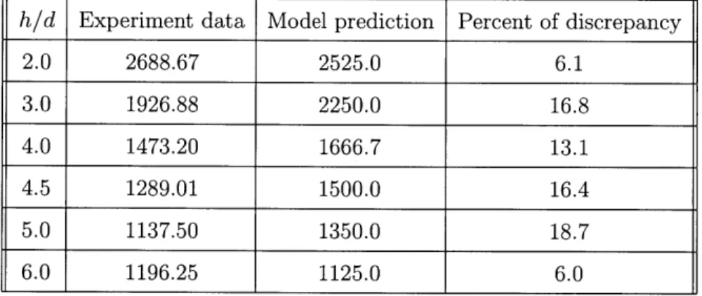
between two tones for different h/d ratios. The result is summarized in Table A.2. It is again encouraging to note that the modelling error relative to the experimental data is less than 20%.

Figs. B-15 and B-19 show the peak frequency intervals between experimental and modelling results at a particular height, h/d = 6.0.

Clearly, Afi and Af2 are comparable in the two figures. It can also be observed

from Table A.2 and Fig. B-19 that the peak interval in both the experimental data and the analytical solution decreases as the height of the lift plate from the ground plane increases from h/d = _{2.0 to h/d = 5.0. This behavior is not observed beyond}

h/d

= _{5.0 and can be attributed to varying dynamics governing the impingement}

tones with height. When the lift plate is close enough to the ground plane, the upstream propagating acoustic waves due to impingement plays a major role in shear layer excitation but its effect diminishes at larger distances. Moreover, the error between the experimental peak interval and predicted one is almost less than 20% at every h/D and is around 6% at heights where the feedback loop is a dominant mechanism in noise generation.

As far as we know, the present work is among the first to obtain analytical mod-els of impingement tones predicting the staging phenomenon and frequency interval magnitudes within tolerable limits. Although the two are not sufficient indicators of the validity of this model, yet the model is considered sufficiently rich and reliable enough to be suitably used as a mathematical model for obtaining control strategy that results in optimal noise reduction.

2.1.4

State-Space Equations

So far, we have sought for a model without microjet control and shown the validity from its ability to predict peak frequency interval for different heights. Regarding the model as a fairly good enough, model-based control strategy still requires a complete state-space equation with well defined input and output factor. One major contribu-tion the microjet can make is velocity change in radial direccontribu-tion near the nozzle exit. Introduction of microjets disturbs the vortex sheet and its effect can be represented

by the modified momentum equation in r-direction (2.23) as follows:

At r = Rj, Z = Znozzle

a

+

a1ap+

- + (Ua + U,(Pp))

_{V_}

₌

(2.31)

where u.1 is the amount of radial directional velocity increase by microjet injection,

P is the supply pressure to microjet.

By separation of variables, we can write for the outer areaQ2 L

p+(r, 6, z, t) = X(t)@i(r, 0, z) (2.32)

where Xi is the state variable, (Di is a set of orthonormal functions satisfying the boundary conditions (Condition 1 Condition 5) and hence can be viewed as the first L modes of the system. Clearly, i

~

is a function of microjet pressure p,,.

Substituting in equation (2.4), and taking inner product with respect to 4i, we get:

i=1

Xis) =2 2@,g(t) ) j= ,- L (2.33)

Since the modes are dependant upon p,, we can write equation (2.32) in vector form as:

X(t) = A(p,)X(t) (2.34)

Discussion about state-space form will stop here. More discrete construction of matrix A(p,,) will be treated at ongoing research. Till now we derived state-space form, essential expression of governing equation, and confirmed that this is different from conventional one in that the control input parameter appears as a parameter in matrix A rather than independent term. The detailed control strategy will be exploited at the next chapter.

2.2

_{Proper Orthogonal Decomposition}

From several different engineering fields, a lot of system's behaviors are governed

by mathematical formula such as ordinary differential equation or partial differential

equation. Many types of physical system are well represented by the solution to these equations. For example, in fluid mechanics field, flow field is fairy well predicted under Navier-Stokes equation. Hence, to get a solution characterizing the detailed motion as close to the real system as possible has been one of the major objective to Fluid mechanics field.

But that is not the sole objective in formulating mathematical model for dynamical system. In case you are trying to control a plat under the real-time condition, solution to a particular case is not meaningful under different situation. Real-time control requires a short calculation time rather than the exact solution. Hence it is needed to sacrifice the correctness of model for making the equation easier to solve and shorten the computation time.

The Proper Orthogonal Decomposition (POD) is a tool used to extract the most energetic modes from a set of realization from the underlying system [17]. These modes can be used as basis functions for Galerkin projections of the model in order to reduce the solution space being considered to the smallest linear subspace that is sufficient to describe the system. The decomposition is 'optimal' in that the energy contained in an N-ordered POD base is greater than any other N-ordered base in a mean-squared sense. Over the years, it has been applied in several disciplines in-cluding turbulence in fluid mechanics, stochastic processes, image processing, signal analysis, data compression, process identification and control in chemical engineering, and oceanography, and has been referred to by various names including Karhunen-Loeve decomposition, principal component analysis, and singular value decomposi-tion. In fluid mechanical systems, the POD technique has been applied in the analysis of coherent structures in turbulent flows and in obtaining reduced order models to describe the dominant characteristics of the phenomena. One of the earliest works was on a fully developed pipe flow, studied by Bakewell and Lumley [6]. Since then,

POD models have been used to model the one-dimensional Ginzburg-Landau equa-tion (Sirovich and Rodriguez [39]), the laminar-turbulent transiequa-tional flow in a flat plate boundary layer (Rempfer [30]), pressure fluctuations surrounding a turbulent jet (Arndt et al. [4]), turbulent plane mixing layer (Delville et al. [10]), velocity field for an axisymmetric jet (Citriniti and George [9]), low-dimensionality of a turbulent flow near wake (Ma et al. [22]), low-dimensional leading-edge vortices in the unsteady flow past a delta wing (Cipolla et al. [8]), and flow over a rectangular cavity (Rowley et al. [31]). The eigenfunctions were developed using both experimental and numerical database.

2.2.1

The Karhunen-Loeve Expansion

Suppose a flow is defined on a spatial domain Q during a time interval T, the flow behaviors such as velocity, trajectory and pressure can be determined from govern-ing equation. These prediction guarantees the accuracy only when the information about boundary condition and initial condition are perfectly given and the governing equation mimics the real system fairly well. But at a certain case the flow field is too sensitive to boundary condition and the small perturbation is not easily detected using a sensor, conventional deterministic flow expression becomes useless. To avoid the unpredictability, the flow is treated as a random process with parameter of time and space. We shall denote the flow variable as follows:

{ut,; t E [0, oo), x E Q} (2.35)

Suppose a flow variable is expressed the sum of orthonormal basis a(t) and O(x),

u(x, t) = 1 an(t)#n(x).

(2.36)

n=1

the complexity of the model can be reduced by truncating the series at a suitable value. There are a large number of basis set to construct the flow, for example equation (2.36). Among these, the Karhunen-Loeve expansion is also one way to

decompose a signal into infinite sum of spatial and temporal term aiming to reduce the complexity.

Mathematically speaking, the flow expanded using the Karhunen-Loeve theorem is stated that,

u(t, x) = F Aan (t)#,(x) (2.37)

n=1

where the temporal terms are uncorrelated

an(t) =( An)1 #n(x)u(t, x)dx

E[am(t)an(t)] = 6, (2.38)

J0#n(x)#n(x)dx = J, (2.39)

and the orthonormal basis functions

{#4}

are calculated from integral equation based on covariance function Ru(x, y)

J

Ru(x, y)#On(y)dy

=

AnOn(x)

x

E Q

R.(x, y) = E[(ux - p (x))(uy - p (y))] (2.40) where p(x), p(y) are mean values of variable ux, uy, respectively and 6n. = 0 (if

m -

n),

1 (if m = n) . The derivation of the temporal term, the uncorrelated property and more rigorous proof can be found in Newman's paper

[25].

2.2.2

Optimality of the Karhunen-Loeve Expansion

Karhunen-Loeve expansion is the optimal linear decomposition method for variables. Here, the "optimal" means that the projection of a variable on the POD mode (ki-netic energy in flow variable sense) is greater than the projection on any other linear decomposition in an average sense for a given number of modes. In other words, Karhunen-Loeve expansion has the least time-averaged error to the original data. Brief explain about optimality will be mentioned here. For the more rigorous proof, it would be better refer to the previous work conducted by Berkooz et al. [7]. If a single

mode

{#}

is said to be "similar" to a variable u, it can be expressed mathematically as follows.

max(I(u, 0) 1) /(0 b) = (I(u,

)

2)/(0, 0) (2.41)

As to Berkooz et al. [7], a necessary condition for the equation (2.41) to hold is that q is an eigenvalue of the two-point correlation function.

J(u(x), u*(x'))#(x')dx' = A#(X') (2.42)

(f, g) =

fa

f(x)g*(x)dx: inner product

( , ): time, space or phase average

R(x, x') = (u(x), u(x')): two-point correlation tensor

Then, the solution

#

satisfying the equation (2.42) will maximize the equation (2.41). But the above eigenvalue problem has infinite number of solutions as long as Q is bounded. We can normalize these eigenfunctions {qk} so that

|I#kJI

= 1 and

order their eigenvalues by An > An 1 - . > 0

If a flow signal u can be decomposed with respect to the POD orthonormal basis

set, it is given by

u(x, t) = Zan(t)#n(x). (2.43)

In Newman's paper [25], it is shown that the mean energy of the flow projected on the a specific mode corresponds to the eigenvalue An

E[l(#, u)12

] = E[I JOn(X)U(t, x)dx2]

= E[J On(x)U(t, x)dxf #n(Y)U(t, y)dy]

= E[J

J

OW(x)u(t, x)qOn(y)u(t , y)dydx]

f

J

(x)E[u(t, x)u(t, y)]#,(y)dydx

J

(x)

J

R(x, y)q5(y)dydx On

~(An

Wq On (x)) dx

= An J qn(x)12dx

= An (2.44)

and the POD coefficient are uncorrelated

(an(t), a* (t)) = 6'An. (2.45) From the above equation (2.44), (2.45) and (2.41), the kinetic energy per unit mass over the domain is denoted by

N N

(u, u*)dx = (a, a*) = E E[l(O, u)12]. (2.46)

n=1 n=1

Suppose the flow signal is expressed from other arbitrary orthonormal set 7,

u(x, t) = Z bn(t) On(X)

j(u,u*)dx

= Z(bn, b*) (2.47)

n

According to the equation (2.41), its energy content projected by a mode

4

is always less than that by POD mode q.

N N N N N

Z(an(t),

a*(t))

=

E[1(0 ,u)1

2

]

=

An

;

E[(Vn,u)1

2

]

= Z(bs(t),

b*(t))

n=1 n=1 n=1 n=1 n=1

(2.48) Therefore, among all linear decompositions, Karhunen-Loeve expansion contains the most energy possible for a given number of modes, which fosters POD method to be used as a good way for reconstructing the model the most efficiently.

There are other approach to explaining the optimality. If F(x, t) is a generalized zero-mean flow variable, then the POD method seeks to generate an approximation for F by using separation of variables as

F(x, t) = T(t)Oi(x) (2.49)

i= 1

where T(t) is the ith temporal mode, Oi(x) is the ith spatial mode, 1 is the number of modes chosen, and t and x are the temporal and spatial variables respectively. The

POD method consists of finding

#i

such that the error F(x, t) - F(x, t) is minimized.

This optimization problem can be stated as follows.

Denote {#i(X)}X=Xe...,2X = 0i E Rn. The POD method is the following

optimiza-tion problem:

min Jm(, ... , 1) = Yj - (Yfqk)k| 2

(2.50)

j=1 k=1

subject to

qi50 = jo, 1 i,j 1,' = [01 . ....

,

Oi (2.51)

where Y E R' is the vector of flow data F at time t = tj.

By definition [43], T is a POD modal set if it is a solution to the optimization

problem (2.50) for any value of 1 K m.

2.2.3

Method of Snapshots

In practice, flow data are measured from a form of discrete signal by a transducer. The analogous form of the Karhunen-Loeve expansion should be calculated from infinite sum of each terms. The procedure for calculating the analogous Karhunen-Loeve expansion is summarized as follows.

1. Let {ui(t)} be a flow variable of a distinct position i at time t

2. The i,

j'th

element of the covariance matrix (R)ij is given by E[ui, uj] and the corresponding orthonormal eigenvector

#

and A are calculated from

R#n = An$ n = 1,2,3 - (2.52)

3. The analogous Karhunen-Loeve expansion and its corresponding temporal term is derived:

ui(t) = EF an(t)(#n)i

n=1

an(t) = ( A)-- Z(#n)iui(t) (2.53)

Above procedure for obtaining analogous Karhunen-Loeve expansion is reasonable but very impractical due to infinite sum. It might cause serious computation problem especially for treating a large number of spatial data. If the number of discrete spatial points might increase, the dimension of the covariance matrix R increases fast that the required computation time to get the eigenvalue also extremely longer. Consider a vary coarse lattice, even 10 x 10 x 10 division renders the 1000 x 1000 size covariance matrix. It is very ineffective in practical points of view. The difficulties associated with large data set should be avoided.

Sirovich [36] in his paper mentioned the method of snapshots, a nice way to make the calculation more simple and the computation less burdensome. Newman [25] showed the detailed derivation of the snapshot method which gives great advantages from the practical points of view. The following is the procedure to get the eigenvec-tors empirically.

Practically, the continuous flow u(t, x) is expressed by u' = u(nw, x) where r is the time interval between data collection. The ergodic hypothesis gives the correlation function as

R(x, y) = lim -j u(X, t)u(y, t)dt (2.54)

T-oo T 0

and in the same manner, for the sufficiently large M, it can be approximated as

R(x, y) - Z ()( )u)(y) (2.55)

M n=1

The integral operator of the approximation becomes

j

(x, y)q5(y)dy

=

J

zu(n)(x)u(")(y)#(y)dy

=-

(x()

J

(n)(y)#5(y)dy

M

= E nu()(x) (2.56)

n==1

From the equation (2.40), this value should satisfy the following

M

Z

a aun() = A#(x) (2.57)