HAL Id: hal-03026304
https://hal.archives-ouvertes.fr/hal-03026304
Submitted on 26 Nov 2020HAL is a multi-disciplinary open access archive for the deposit and dissemination of sci-entific research documents, whether they are pub-lished or not. The documents may come from teaching and research institutions in France or abroad, or from public or private research centers.
L’archive ouverte pluridisciplinaire HAL, est destinée au dépôt et à la diffusion de documents scientifiques de niveau recherche, publiés ou non, émanant des établissements d’enseignement et de recherche français ou étrangers, des laboratoires publics ou privés.
The RESOLVE project: a multi-physics experiment with
a temporary dense seismic array on the Argentière
Glacier, French Alps
Florent Gimbert, Ugo Nanni, Philippe Roux, A. Helmstetter, S. Garambois,
A. Lecointre, A. Walpersdorf, B. Jourdain, M. Langlais, O. Laarman, et al.
To cite this version:
Florent Gimbert, Ugo Nanni, Philippe Roux, A. Helmstetter, S. Garambois, et al.. The RESOLVE project: a multi-physics experiment with a temporary dense seismic array on the Argentière Glacier, French Alps. Seismological Research Letters, In press. �hal-03026304�
1
The RESOLVE project: a multi-physics experiment with a temporary
1
dense seismic array on the Argentière Glacier, French Alps
2 3
Gimbert, F.1, U. Nanni1, P. Roux2, A. Helmstetter2, S. Garambois2, A. Lecointre2, A. 4
Walpersdorf2, B. Jourdain1, M. Langlais2, O. Laarman1, F. Lindner3, A. Sergeant4, C. Vincent1, F. 5
Walter3 6
7 8
1 University Grenoble Alpes, CNRS, IRD, IGE, Grenoble, France 9
2 University Grenoble Alpes, CNRS, IRD, UGE, ISTerre, Grenoble, France 10
3 Laboratory of Hydraulics, Hydrology and Glaciology, ETH Zürich, Zürich, Switzerland 11
4 Aix Marseille Univ, CNRS, Centrale Marseille, LMA, France 12
13 14
ABSTRACT 15
Recent work in the field of cryo-seismology demonstrates that high frequency (>1 Hz) seismic 16
waves provide key constraints on a wide range of glacier processes such as basal friction, 17
surface crevassing or subglacial water flow. Establishing quantitative links between the 18
seismic signal and the processes of interest however requires detailed characterization of the 19
wavefield, which at high frequencies necessitates the deployment of large and particularly 20
dense seismic arrays. Although dense seismic array monitoring has recently become 21
increasingly common in geophysics, its application to glaciated environments remains limited. 22
Here we present a dense seismic array experiment made of 98 3-component seismic stations 23
continuously recording during 35 days in early spring 2018 on the Argentière Glacier, French 24
Alps. The seismic dataset is supplemented with a wide range of complementary observations 25
obtained from ground penetrating radar, drone imagery, GNSS positioning and in-situ 26
measurements of basal glacier sliding velocities and subglacial water discharge. We present 27
first results through conducting spectral analysis, template matching, matched-field 28
processing and eikonal wave tomography. We report enhanced spatial resolution on basal 29
Manuscript Click here to
2
stick slip and englacial fracturing sources as well as novel constraints on the heterogeneous 30
nature of the noise field generated by subglacial water flow and on the link between crevasse 31
properties and englacial seismic velocities. We outline in which ways further work using this 32
dataset could help tackle key remaining questions in the field. 33
34
INTRODUCTION 35
The deployment of large and dense seismic arrays is becoming increasingly common in various 36
geophysical contexts thanks to new technological developments of autonomous wireless 37
seismographs and increased computational power. Spatially dense arrays enhance the 38
characterization of high frequency (>1 Hz) body and surface waves propagating in the 39
subsurface, such as for example in near-surface fault systems exhibiting hundreds to few tens 40
of meters long structures (e.g., the Newport-Inglewood Fault, see Lin et al. (2013), and the 41
San Jacinto Fault, see Roux et al. (2016)). The improved resolution provided by dense arrays 42
increases the completeness of impulsive seismic event catalogs (Vandemeulebrouck et al., 43
2013), thus allowing source spatio-temporal dynamics and subsurface structure to be studied 44
in greater details (Meng and Ben-Zion, 2018; Chmiel et al., 2019). Dense arrays also help to 45
detect other sources of radiation (e.g. tremor and anthropogenic sources) compared to what 46
is possible with single stations or regional networks (Inbal et al., 2016; Li et al., 2018; Meng 47
and Ben-Zion, 2018). Despite its strong potential, dense array monitoring is still limited in the 48
study of glaciers, although it could be used to address some of the key open questions in the 49
field of glaciology. 50
51
Glaciers exhibit damage zones created by surface and/or basal crevasses (Walter et al., 2015; 52
Lindner et al., 2019; Zhan, 2019; Sergeant et al., 2020) as well as complex three dimensional 53
3
structures associated with firn/debris layers, bedrock topography or englacial water conduits 54
(Cuffey and Paterson, 2010). These features are known to undergo large spatial and temporal 55
changes and to play an important role in glacier dynamics and thermo-dynamics (Durand et 56
al., 2011; Scherler et al., 2011; Gilbert et al., 2020). However, conventional geophysical
57
techniques such as radar sounders capable of resolving englacial structural features (e.g., 58
Evans and Robin, 1966; Church et al., 2019) are not suited for evaluating detailed spatial and 59
temporal changes as well as their effects on the overall glacier behavior. Instead, active and 60
passive surveys using dense seismic arrays may enable accurately monitoring these changes 61
(e.g. using englacial seismic velocities, see Lindner et al. (2019) and Preiswerk et al. (2019)) 62
and thus yield unprecedent constraints on glacier structure and temporal evolution. 63
64
Glaciers and ice sheets generate a large variety of seismic signals, from impulsive transients 65
to emerging and sustained tremors (Podolskiy and Walter, 2016; Aster and Winberry, 2017). 66
Impulsive arrivals from basal stick-slip events have been observed in numerous glaciological 67
contexts (Weaver and Malone, 1979; Allstadt and Malone, 2014; Helmstetter, Nicolas, et al., 68
2015; Lipovsky and Dunham, 2016; Lipovsky et al., 2019; Walter et al., 2020) and may yield 69
crucial information on glacier basal motion, which exerts a primary control on glacier and ice-70
sheet dynamics and the associated eustatic sea level rise (Ritz et al., 2015; Vincent and 71
Moreau, 2016). The mechanisms giving rise to stick-slip sliding as well as its effect on large-72
scale ice flow, however, remain poorly constrained (Lipovsky et al., 2019). Dense array 73
monitoring could allow improving the detection of stick-slip events, yield more accurate 74
inversions of locations and show if and how fast stick-slip asperities migrate. 75
4
Impulsive events from englacial fracturing are also commonly observed (Neave and Savage, 77
1970; Roux et al., 2010; Mikesell et al., 2012; Podolskiy et al., 2018; Garcia et al., 2019), and 78
may help elucidate the role of crevassing in iceberg calving, the disintegration of ice-shelves 79
and the occurrence of serac falls (Faillettaz et al., 2008; Krug et al., 2014; Lipovsky, 2018). The 80
improved detection and resolution provided by dense arrays could provide novel constraints 81
on crevasse depth and rupture propagation rates, which are needed to test models (van der 82
Veen, 1998; Weiss, 2004; Tsai and Rice, 2010) and thus better understand ice sheet integrity. 83
84
Recent seismic investigations have also reported widespread emergent and sustained tremor 85
signals generated by resonances in moulins or water-filled crevasses (Helmstetter, Moreau, et 86
al., 2015; Roeoesli et al., 2016; Aso et al., 2017), subglacial water flow (Bartholomaus et al.,
87
2015; Eibl et al., 2020; Lindner et al., 2020; Nanni et al., 2020) and subglacial sediment 88
transport (Gimbert et al., 2016). The possibility to calculate physical characteristics of 89
subglacial water flow as well as of subglacial sediment transport from seismic tremor 90
observations (Tsai et al., 2012; Gimbert et al., 2014, 2016; Bakker et al., 2020) is particularly 91
appealing. These processes play an important role in ice sliding speeds (Zwally et al., 2002; 92
Schoof, 2010; Tedstone et al., 2015) and bedrock erosion (Beaud et al., 2016), and yet 93
hydraulic measurements at the ice bed are notoriously difficult, with traditional approaches 94
such as borehole techniques providing point measurements, only (e.g., Iken and Bindschadler, 95
1986; Iken et al., 1993). Theoretical links between discharge, pressure regime, sediment 96
transport rates and geometry of the subglacial drainage system and seismogenic hydraulic 97
noise sources remain to be more fully tested and dense seismic arrays may provide the 98
necessary spatial extent and resolution for doing so. 99
5
Properly evaluating the knowledge gain that dense seismic arrays may provide to address the 101
above-mentioned challenges requires (i) monitoring a glacier that gathers the processes of 102
interest, (ii) deploying instrumentation that covers scales and durations over which significant 103
changes operate, and (iii) acquiring complementary observations to test the seismically-104
derived findings and incorporate these into a wider glaciological context. Here we present 105
data and first analysis from a 98 sensor array deployed over 35 days during early spring 2018 106
on an Alpine Glacier, the Argentière Glacier in the French Alps (Fig. 1). We also provide and 107
analyze key complementary observations from Ground Penetrating Radar (GPR), drone 108
imagery, Global Navigation Satellite System (GNSS) positioning and in-situ instrumentation of 109
basal glacier sliding velocities and subglacial water discharge. We argue that the selected 110
glacier, the time period of investigation as well as the completeness of the present dataset 111
satisfies all of the three above-mentioned conditions. Through application of spectral analysis, 112
template matching, matched-field processing and eikonal wave tomography, we demonstrate 113
that use of the present dataset enhances spatial resolution of basal stick slip activity and near 114
surface crevassing. We further provide novel constraints on the degree of heterogeneity of 115
the seismic noise field generated by subglacial water flow and the variations of englacial 116
seismic velocities. We finally outline how future work using this dataset could help overcome 117
classical observational limitations and address key challenges in the field. 118 119 EXPERIMENT DESIGN 120 121 FIELD SITE 122 123
The Argentière Glacier is located in the Mont Blanc Massif (French Alps, 45°55’ N, 6°57’E, Fig. 124
1a) and is the second largest French glacier. It is about 10 km long, covers an area of about 12 125
6
km2, extends from an altitude of 1700 m above sea level (a.s.l.) up to about 3600 m a.s.l. with 126
an equilibrium line altitude at about 2900 m a.s.l. (Vincent et al., 2018). Over the past three 127
decades, glacier total mass balance has been negative (0.7 meter water equivalent loss per 128
year on average over the period 1976-2019), glacier snout has been retreating by several 129
hundreds of meters (815 m retreat between 1990 and 2019), glacier surface elevation has 130
decreased by several tens of meters and glacier surface velocities have decreased by about a 131
factor of two in the ablation zone (Vincent et al., 2009). The upper part of the glacier is 132
constricted in a typical U-shaped narrow valley where ice sits on granite. The lower part of the 133
glacier is characterized by a sharper incised, V-shaped valley where ice sits on metamorphic 134
rocks (Vallon, 1967; Hantz and Lliboutry, 1983; Vincent et al., 2009). The glacier generally 135
exhibits temperate bed conditions (Vivian and Bocquet, 1973), i.e. basal ice temperature is at 136
the pressure melting point and water flow occurs at the interface as a result of year-round 137
basal melt and summer surface melt (Cuffey and Paterson, 2010). 138
139
The monitored site is located in the lower part of the glacier (about 2 km from the glacier 140
front) and at about 2400 m a.s.l. (Fig. 1b). In this area the surface slope is gentle (1-2%) and 141
crevasses are restricted to an area of about 200 m from the glacier sides. The glacier flows at 142
a yearly average velocity of about 60 m.yr-1 in its center, about half of which is due to sliding 143
at the ice-bed interface and the other half to internal ice deformation (Vincent and Moreau, 144
2016). Internal ice deformation likely occurs primarily through ice creep except near the 145
glacier sides where crevasses are large and potentially deep, such that englacial fracturing 146
could also play a role. A strong seasonality is observed in glacier dynamics, with summer 147
(typically May to September) velocities equal to about 1.5 times winter velocities (Vincent and 148
7
Moreau, 2016). This behavior is known to result from melt water input lubricating the ice-bed 149
interface and enhancing basal sliding (Lliboutry, 1959, 1968; Cuffey and Paterson, 2010). 150
Previous seismic observations at this site report various seismogenic sources associated with 151
surface and intermediate depth crevassing (Helmstetter, Moreau, et al., 2015), basal stick-slip 152
(Helmstetter, Nicolas, et al., 2015), subglacial water flow (Nanni et al., 2020), and serac 153
instabilities in the glacier front (Roux et al., 2008). 154
155
SEISMIC INSTRUMENTATION AND GEOPHYSICAL CHARATERISATION OF GLACIER STRUCTURE 156 AND DYNAMICS 157 158 Seismic instrumentation 159 160
Sensors of the dense seismic array (red dots in Fig. 1b) are Fairfield ZLand 3-component nodal 161
seismographs with a sampling frequency of 500 Hz (hereafter referred to as nodes). These 162
sensors have a low-corner cut-off frequency of 5Hz, a sensitivity of 76.7 V.m-1.s-1 (see Ringler 163
et al. (2018) for a detailed laboratory analysis of sensor response characteristics) and a typical
164
power autonomy of about 35 days. We deployed the nodes on 24 April 2018 when the glacier 165
was entirely covered by a snow layer of about 3 m thick. We placed the sensors about 40 m 166
apart from each other in the along-flow direction and about 50 m apart in the across-flow 167
direction in order to enable subwavelength analysis in the 4-50 Hz frequency range of interest. 168
Given that snow melt occurs at an average rate of 2-4 cm.day-1 water equivalent at this 169
location (Vincent and Moreau, 2016), we decided to bury the nodes into snow about 30 cm 170
below the surface to ensure the sensors be (i) well coupled to their surroundings and 171
maintained levelled over a week-long time period until snow melt uncovered them and (ii) 172
8
shallow enough for the GNSS signal to pass through the snow layer and ensure proper 173
reception for time synchronization. Given the limited melt that occurred over the first half of 174
the monitoring period, we had to re-bury the sensors only once over the monitored period, 175
on 11 May 2018. This strategy ensured that little data was lost due to melt-out-induced tilt. 176
177
We supplemented the seismic array with one three-component borehole seismic station 178
placed at 5 m below the ice-surface (orange dot in Fig. 1b). This Geobit-C100 sensor was 179
connected to a Geobit-SRi32L digitizer and provides higher sensitivity (1500 V.m-1.s-1), higher 180
frequency sampling (1000 Hz) and a lower low-corner cut-off frequency (0.1 Hz) compared to 181
the nodes. This seismic station is the same as the one used for the two-year long seismic study 182
of Nanni et al. (2020). 183
184
Recovery of surface and bed digital elevation models from structure from motion surveys 185
and ground penetrating radar 186
187
We construct a digital surface elevation model based on a drone geodetic survey that we 188
conducted on September 5, 2018 when the glacier surface was snow free and crevasses could 189
be identified. We used a senseFly eBee+ Unmanned Aerial Vehicle and acquired a total of 720 190
photos using the onboard senseFly S.O.D.A. camera (20 Mpx RGB sensor with 28 mm focal 191
lens). We generate a digital elevation model of 10-cm resolution (see white contours in Fig. 192
1b) using differential Global Positioning System (GPS) measured ground control points (see 193
green stars in Fig. 2a) and the Structure for Motion algorithm implemented in the software 194
package Agisoft Metashape Professional version 1.5.2. A detailed description of the 195
processing steps can be found in Brun et al. (2016) and Kraaijenbrink et al. (2016). 196
9 197
We calculate a crevasse map (black dots in Fig. 2a) based on the surface digital elevation 198
model, which has been shown to be more reliable and precise than using optical/radar images 199
(Foroutan et al., 2019). We first apply a 2D highpass filter with a low cut-off wavelength of 10 200
m and then define any location with elevation lower than -50 cm as being part of crevasses. 201
Finally, we apply a 2D median filter with a 1 by 1 m kernel in order to remove artifacts from 202
boulders and moraines. 203
204
To establish a digital elevation model of the glacier bed we primarily use Ground Penetrating 205
Radar (GPR) data acquired using a system of two transmitting and receiving 4.2 MHz antennas 206
connected to a time triggered acquisition developed especially for glacial applications by the 207
Canadian company Blue System Integration Ltd (Mingo and Flowers, 2010). The GPR signal 208
processing consists of correcting for source time excitation. We use both dynamic corrections 209
to reproduce a zero-incidence acquisition from data acquired with a 20 m offset between 210
source and receiver (Normal Moveout correction) and static corrections to highlight elevation 211
variations along a profile. We do so using a constant wave velocity of 0.168 m.ns-1 that is 212
typical for ice (Garambois et al., 2016). We then apply a [1-15 MHz] Butterworth band-pass 213
filter followed by a squared time gain amplification to the signal in order to increase signal-to-214
noise ratio. We show an illustration of the processed GPR data in Fig. 2b, where the direct air-215
wave first arrival is followed by a large reflectivity V-shape pattern reaching 3000 ns around 216
the center of the profile. This latter profile corresponds to the ice/bedrock interface, although 217
its apparent shape is biased by reflections off the closest point on the ice-bed interface rather 218
than off the bed portion directly below the instrument. We correct for this bias by applying a 219
frequency-wavenumber Stolt migration technique (Stolt, 1978) and convert time into distance 220
10
using the constant wave velocity of 0.168 m.ns-1. We note that prior to migration we add null 221
traces (i.e. with null amplitudes) in places where harsh glacier surface conditions (mainly 222
crevasses) prevented us from acquiring data. As illustrated in Fig. 2c the migration process is 223
effective in correcting the artefacts due to the geometrical variation of the interface along the 224
profile, which now appears smooth and continuous. We then pick the ice-bed reflection 225
(yellow line in Fig. 2c) over all GPR profiles, such that a three-dimensional bed DEM can be 226
reconstructed. 227
228
We reconstruct a three-dimensional bed DEM over a larger area than that covered by GPR 229
surveys by incorporating additional constraints like glacier edge elevation as measured from 230
drone imagery (blue area in Fig. 2a) and bed elevations obtained through rock drilling to the 231
ice-bed interface from bedrock excavated tunnels located further down-glacier (purple area 232
in Fig. 2a). Furthermore, we interpolated all data using a kriging method onto a 10 by 10 m 233
grid. From different first onset pickings we estimate that the recovered depth uncertainty is 234
of about 5 m below the seismic array and likely on the order of a few tens of meters outside 235
of the array where observations are sparser. 236
237
In Fig. 2a we show the ice thickness map (using 25-m bin contours) as reconstructed based on 238
subtracting the bed DEM from the surface DEM. The glacier bed exhibits a gently dipping 239
valley, with a maximum ice thickness of about 255 m at the center of the seismic array. Glacier 240
thickness decreases relatively sharply on the glacier margins where surface crevasses are 241
observed. We also observe that bed elevation significantly increases down glacier, which 242
results in a decrease by more than 150 m in glacier thickness (Fig. 2d). Beyond these generic 243
characteristics we identify two interesting reflectivity features in the migrated GPR images 244
11
(yellow ellipses in Fig. 2c) that correspond to localized scattering observed near the surface 245
and a large reflectivity pattern observed just above the deepest portion of the interface. The 246
near surface scattering feature could be caused by deep crevasses, and the deeper feature 247
could be caused by englacial and/or subglacial water conduits as recently proposed by Church 248
et al. (2019), who made similar GPR observations in a temperate glacier and were able to
249
bolster their interpretation with in-situ borehole observations. 250
251
Meteorological and water discharge characteristics 252
253
We use air temperature and precipitation measurements obtained at a 0.5 h time step with 254
an automatic weather station maintained by the French glacier-monitoring program 255
GLACIOCLIM (Les GLACIers un Observatoire du CLIMat; https://glacioclim.osug.fr/), which is 256
located on the moraine next to the glacier at 2400 m a.s.l. (green diamond in Fig. 1b). 257
Precipitation is measured with an OTTPluvio weighing rain gauge. Subglacial water discharge 258
is monitored at a 15 min time step in tunnels excavated into bedrock by the Emossons 259
hydraulic power company, which are located 600 m downstream of the array center (at 2173 260
m a.s.l.) near the glacier ice fall (see blue star in Fig. 1b). 261
262
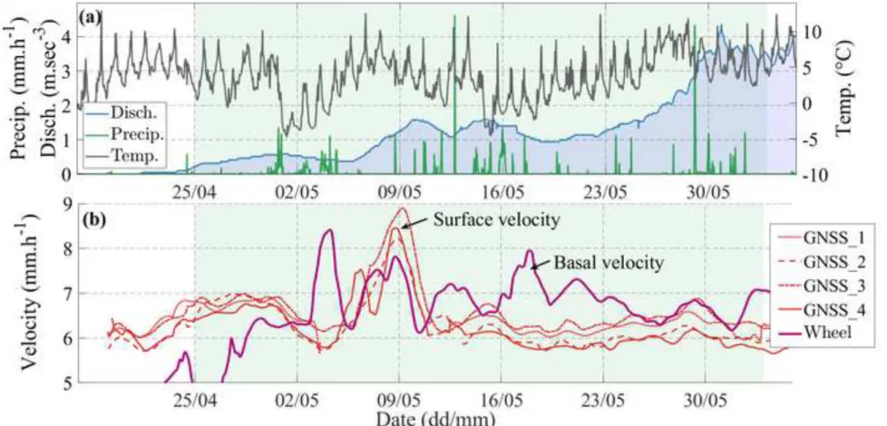
Temperature generally increases over the instrumented period, from a multi-daily average of 263
about 0° C at the beginning of the measurement period to about 5 °C at the end (Fig. 3a). This 264
drives the general increase in water discharge, which varies from few tenths of m3.s-1 to 265
several m3.s-1 over the period. Episodic rain events also occur during the instrumented period, 266
but have little to no effect on subglacial discharge likely as a result of the snow cover acting as 267
a water storage buffer (Fountain and Walder, 1998). 268
12 269
Glacier dynamics instrumentation and general features 270
271
We evaluate changes in glacier dynamics over the instrumented period by means of two 272
observational methods. The first one is unique to the present site, and consists of basal sliding 273
velocity measurements made continuously in the down glacier serac fall area (see red star in 274
Fig. 1b) by means of a bicycle wheel placed directly in contact with the basal ice at the 275
extremity of an excavated tunnel (Vivian and Bocquet, 1973; Moreau, 1999). The wheel is 276
coupled with a potentiometer that retrieves its rotation rate, which is then recorded digitally 277
and converted back to a sliding velocity at a 1-s sampling time with a displacement increment 278
resolution of 0.07 mm. The second type of measurements consists of 4 glacier surface and 1 279
reference bedrock GNSS stations (yellow stars in Fig. 1b) of type Leica GR25 acquiring the GNSS 280
signals every second. This temporary array is supplemented by a permanent ARGR GNSS 281
station from the RESIF-RENAG network (http://renag.resif.fr) on the bedrock close to the 282
glacier 3 km uphill (yellow star in Fig. 1a). The GNSS antennas on the glacier are installed on 283
8-m long aluminum masts anchored 4-m deep in the ice and thus emerging about a meter 284
above the snow surface at the beginning of the measurement period. The temporary station 285
placed next to the glacier side provides a reference for validating kinematic GNSS processing 286
approaches, evaluating station positions from every single set of GNSS signal recordings (i.e. 287
every second, as opposed to static processing, which cumulates GNSS signals over a much 288
longer time). We conduct such kinematic processing using the TRACK software ((Herring et al., 289
2018), http://geoweb.mit.edu/gg/docs.php). Our processing chain includes the on-line tool 290
SARI (https://alvarosg.shinyapps.io/sari/) for the removal of outliers that arise from low 291
satellite coverage in the glacier valley and to perform a de-trend and re-trend analysis to 292
13
estimate and correct for offsets due to manual antenna mast shortening as snow melt 293
progresses. We also correct for multi-path effects induced by GNSS signal reflections from the 294
ground, although we find that those are attenuated by the combination of GPS and GLONASS 295
signals thanks to their different sidereal periods (~24 h for GPS and ~8 days for GLONASS). We 296
finally calculate position time series at a 30-s time step sufficient to capture glacier dynamics 297
and subsequently evaluate three-dimensional velocities by the linear trends of the position 298
components. The horizontal velocity is calculated as 𝑣ℎ = √𝑣𝑁2 + 𝑣𝐸2 where 𝑣𝑁 and 𝑣𝐸 are
299
the North and East components, respectively. 300
301
To facilitate comparison of basal sliding and surface velocity here we smooth both timeseries 302
at a 36-hr timescale (Fig. 3b), since daily down to sub-daily fluctuations in basal sliding 303
velocities are largely affected by unconstrained variations in the local ice roughness in contact 304
with the wheel, as for example, when an entrained rock passes over the wheel. Although basal 305
sliding velocity is to be lower than surface velocity, here both quantities have similar absolute 306
values because the sliding velocity is measured at a place where the glacier is much steeper 307
(25% slope as opposed to 1-2%) and thus driving stress is much larger than at the GNSS 308
locations. We observe an increase in basal sliding velocity from 4.5 mm/h to more than 6 309
mm/h at the very beginning of the monitored period. Such an acceleration is commonly 310
observed in spring on alpine glaciers (Iken and Bindschadler, 1986; Mair et al., 2002; Vincent 311
and Moreau, 2016) and is known to correspond to water pressurization caused by an increase 312
in water input at the bed due to surface melt water supply, which causes the reduction of 313
friction and thus the enhancement of sliding (Lliboutry, 1959, 1968; Iken, 1981; Schoof, 2005; 314
Gagliardini et al., 2007). This acceleration is not seen in the GNSS observations, which could 315
be due to the glacier seasonal acceleration occurring earlier at this location. We also observe 316
14
one major acceleration event in the location of the dense seismic array occurring between 4 317
May and 8 May 2018 likely due to the large concomitant increase in water discharge (see 318
blue line in Fig. 3a) causing basal water pressurization (Cuffey and Paterson, 2010). 319 320 321 FIRST RESULTS 322 323
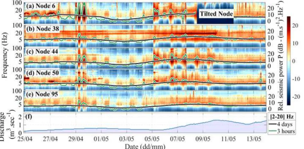
SEISMIC NOISE CHARACTERISTICS 324
325
We investigate the spatial and temporal variability of seismic power 𝑃 (in dB) across a wide 326
range of frequencies by applying Welch’s method (Welch, 1967) over 4 seconds-long vertical 327
ground motion timeseries (with 50 % overlap) prior to averaging power (in the decibel space) 328
over 15 minutes-long time windows. This two-step strategy allows limiting the influence of 329
impulsive events (which are studied in more details in the next sections) on the seismic power 330
while enhancing that of the continuous background noise (Bartholomaus et al., 2015; Nanni 331
et al., 2020). In Fig. 4 we present 1-100 Hz spectrograms (i.e. seismic power at any given
332
frequency and time) over the first half of the instrumented period (15 April to 14 May 2018) 333
together with timeseries of 2-20 Hz frequency median seismic power at five different stations 334
of the array, four stations located on the four array sides and one located in the array center 335
(see node numbers in Fig. 1b and Fig. S1 for spectrograms across all stations and over the 336
entire frequency range and experimental period). Time periods when sensors tilted beyond 337
their specifications (and thus were no longer deemed functional) as a result of snow melt 338
causing them to be no longer buried are manifested by drastically reduced seismic power 339
across the whole frequency range (see node 6 from 8 May to 11 May 2018). Fortunately, 340
15
sensor tilt only occurred at a small number of seismic stations (11 out of 98) and during a 341
restricted time duration (less than 2 days on average, see Fig. S1). We also observe that 342
spectrograms do not undergo significant change from prior to after sensor reinstallation on 343
11 May 2018. This suggests that these are not significantly affected by potential changes in 344
sensor coupling to snow, which is pleasant given that a previous study found that coupling can 345
strongly affect nodes recorded signals (Farrell et al., 2018). 346
347
All stations generally experience similar multi-day (e.g. four days’ average, see black lines in 348
Fig. 4) variations in seismic power that are highly correlated with multi-day discharge 349
variations, although seismic power precedes discharge variations by about a day or two. The 350
likely reason is that seismic power is controlled by the hydraulic pressure gradient, which is 351
highest during periods of rising discharge (Gimbert et al., 2016; Nanni et al., 2020). Although 352
shorter term (e.g. diurnal) variations in seismic power are also similar across stations when 353
discharge is low (from 24 April to 28 April and from 30 April to 4 May) and anthropogenic noise 354
dominates (Nanni et al., 2020), the picture is different at higher discharges when seismic 355
power is dominated by subglacial water flow (Nanni et al., 2020). On 29 April and from 5 May 356
to 10 May seismic power exhibits pronounced (up to 10 dB) and broad frequency (1-100 Hz) 357
short time scale (sub-diurnal to diurnal) variations that are particularly marked at certain 358
stations (e.g. node 6 (Fig. 4a), node 44 (Fig. 4c) and node 50 (Fig. 4d)) and not at others (e.g. 359
node 38 (Fig. 4b) and 95 (Fig. 4e)). We also observe that at certain stations seismic power 360
appears to be continuously or intermittently enhanced within narrow frequency bands. For 361
instance node 38 systematically presents higher seismic power above 20 Hz. These 362
discrepancies suggest that measurements of ground motion amplitude are sensitive to 363
heterogenous and intermittent subglacial water flow, although certain features discussed 364
16
here could be due to extraneous noise sources associated with sensor coupling (Farrell et al., 365
2018), to localized sources other than subglacial fluid flow or to site effects. 366
367
DETECTING AND LOCATING BASAL STICK SLIP IMPULSIVE EVENTS USING TEMPLATE 368
MATCHING 369
370
We detect high-frequency (>50 Hz) basal stick-slip events using template matching. This 371
follows a two-step analysis as in Helmstetter et al. (2015). We first build a catalog of events 372
through applying a short-term-average over long-term-average (STA/LTA) detection method 373
(Allen, 1978) to the continuous high-pass filtered signal (>20 Hz) using a STA time window of 374
0.1 s and a LTA time window of 1 s. We identify an event when the STA/LTA ratio exceeds a 375
factor of 2. We then manually select all events with short duration (<0.2 s) and high average 376
frequency (>50 Hz) and define groups of events referred to as clusters when their correlation 377
with each other exceeds 0.8. For each cluster, we compute the average waveform to define 378
its “template” signal (using a time window of 0.25 s). We take the sum of seismograms 379
normalized by their peak amplitude and weighted by the square correlation between each 380
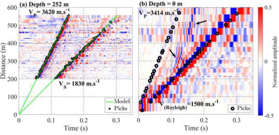
event and the template event, iterating this procedure several times until convergence. We 381
visually check that events present distinct P and S wave arrivals and use a polarization analysis 382
to ensure that they are not associated with surface waves (Fig. 5a). We then use the template 383
matching filter method (Gibbons and Ringdal, 2006) to further detect smaller amplitude 384
events not picked with the above strategy but exhibiting a correlation higher than 0.5 with the 385
template signal. 386
17
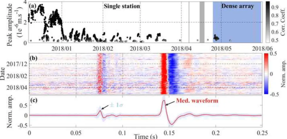
We first conduct the analysis using the borehole station ARG, which has a higher sensor 388
sensitivity, signal-to-noise and sampling rate compared to the nodes. We identify 31 active 389
clusters during the dense array experiment. Interestingly, these clusters constitute a large part 390
of the 46 clusters identified on a much longer period (from December 2017 to June 2018, using 391
the borehole sensor which ran almost continuously, see Fig. 6). Although the amplitude of 392
these signals varies strongly through time (from 1 ⋅ 10−7 m.s-1 to 4 ⋅ 10−6 m.s-1 Fig. 6a), 393
waveform characteristics remain strikingly similar (Fig. 6b and 6c). All 46 identified clusters 394
exhibit similar characteristics to that shown in Fig. 6, and their activity does not appear to be 395
temporally correlated with each other, nor with external drivers related to meteorology, 396
hydrological or glacier dynamics. 397
398
We also apply the template matching algorithm on a subset of 10 nodes covering the whole 399
study area, using the same 31 clusters as previously identified using station ARG. At each time 400
step we compute the correlation coefficient between each template signal and the continuous 401
signal averaged over all nodes and all components (using a time window of 0.35 s instead of 402
0.25 s in order to match signal duration at all selected nodes). The large number of sensors 403
allows us to lower the correlation threshold from 0.5 to 0.2 while reducing the number of false 404
detections. Indeed, events belonging to different clusters with very different locations can end 405
up being correlated above the detection threshold when using one station, while using several 406
stations this scenario is much more unlikely. We detect 79% more events using the nodes 407
compared to using the station ARG. The newly detected events are mostly smaller amplitude 408
events. Most (83%) of the events detected using ARG are also detected using the nodes. This 409
shows that increasing the number of sensors allows detecting more events and reducing the 410
number of false detections despite signal-to-noise ratio and sampling rate not being optimum. 411
18 412
We determine the position of the 31 identified clusters by first manually picking on each node 413
the P and S arrival times associated with the event in each cluster that is associated with the 414
largest correlation with the template event, and then inverting for the location of each event 415
and the associated P and S wave velocities assuming velocities are homogeneous and identical 416
for all events. We only consider first arrivals that are usually geometrically predicted to be 417
direct (as opposed to refracted) waves for most sensors and most events. Assuming a simple 418
1D velocity model with 𝑉𝑃=3620 m/s in the ice and 𝑉𝑃=4300 m/s in the bedrock (see Fig 10b)
419
and a glacier thickness of 200 m, the direct wave is faster for epicentral distances shorter than 420
306 m. Moreover, even when the refracted wave is faster, it is usually less impulsive and has 421
a smaller amplitude than the direct wave. We estimate P and S wave velocities using a grid 422
search inversion with a step of 10 m.s-1 and the Nonlinloc software (Lomax et al., 2000) to 423
locate clusters. We assume a standard error of arrival times of 2 ⋅ 10−3 s for P waves, 4 ⋅ 10−3s 424
for S waves and of 3.5 ⋅ 10−3 s for calculated travel times. We can see in Fig. 5a that the picked 425
arrival times (black circles) are consistent with the computed travel times (green lines). The 426
root-mean-square error for this event is 2.4 ms, which corresponds to about one sample (2 427
ms). 428
429
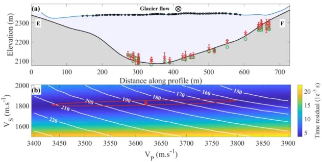
We show the locations of basal icequakes versus depth in an average transverse section in Fig. 430
7a and on a two-dimensional map in Fig. 8. They are mainly located in the down-glacier part 431
of the array and in the central part of the glacier or near the right side, while there is no event 432
observed towards the left side. Icequake depths range between 80 m and 285 m, and are in 433
good agreement with the bedrock topography estimated from the radar profiles. Uncertainty 434
on absolute source depth is on the order of 10 m (see errorbars in Fig. 7a), and the estimated 435
19
seismic wave velocities of 𝑉𝑃=3620 m.s-1 and 𝑉𝑆=1830 m.s-1 (Fig. 7b) are in good agreement
436
with velocities measured on other alpine glaciers (Podolskiy and Walter, 2016). 𝑉𝑆 is much
437
better constrained by the data compared to 𝑉𝑃 (Fig. 7b).
438 439
SYSTEMATIC LOCATION OF EVENTS USING MATCHED-FIELD PROCESSING 440
441
Contrary to in the previous section where a priori constraints on waveform characteristics and 442
wave velocity are used to target basal stick-slip events, we next test location of a wide range 443
of seismic events generated by impulsive or emergent sources with no a priori knowledge on 444
waveform characteristics and minimal a priori knowledge on medium properties. The 445
rationale is that the limited a-priori knowledge for source identification is balanced by the high 446
spatial and temporal resolution provided by array processing techniques, which may provide 447
spatial or temporal characteristics facilitating source identification (Vandemeulebrouck et al., 448
2013; Chmiel et al., 2019). 449
450
We conduct Matched-Field Processing (MFP), which consists of recursively matching a 451
synthetic field of phase delays between sensors with that obtained from observations using 452
the Fourier transform of time-windowed data. We obtain the synthetic field from a source 453
model with a frequency-domain Green’s function that depends on 4 parameters, which are 454
the source spatial coordinates 𝑥, 𝑦 and 𝑧 and the medium phase speed 𝑐. MFP output is 455
normalized to range from 0 to 1 with higher values corresponding to better matches between 456
modelled and observed signal phases, and therefore a higher confidence in true source 457
location. Here we use a spatially homogeneous velocity field within the glacier, which the 458
advantage of a fast-analytical computation, although it also results in a higher degree of 459
20
ambiguity between 𝑧 and 𝑐. Contrary to classical beamforming techniques in which a planar 460
wave front is often assumed, our MFP approach considers spherical waves and allows locating 461
sources closer to and within the array. To build a large catalog of events, we apply MFP over 462
short time windows of 1-s with 0.5-s overlap, across 16 frequency bands of ±2 Hz width equally 463
spaced from 5 to 20 Hz and over the entire study period. Calculating source locations over 464
such a large number of windows requires minimizing computational cost. We do so by using 465
a minimization algorithm that relies on the downhill simplex search method (Nelder-Mead 466
optimization) of Nelder and Mead (1965) and Lagarias et al. (1998) instead of using a multi-467
dimensional grid search approach. As the exploration of the solution space is characterized by 468
a certain level of randomness, we maximize the likelihood that our minimization technique 469
finds a global minima and thus the dominant source over the considered time window through 470
(i) starting the optimized algorithm from a set of 29 points located at a depth of 250 m inside 471
and near the array (see black crosses in Fig. 9d) with a starting velocity 𝑐=1800 m.s-1 and (ii) 472
taking the highest MFP output out of the 29 inversions found after convergence. 473
474
In Fig. 9b,c we present two examples of events located inside and outside the array and 475
associated with a high MFP output of 0.92. The half-size of the focal spot in the MFP output 476
field gives a measure of the location uncertainty (Rost and Thomas, 2002), which is about 10 477
m for events located inside the array and can increase up to 40 m when for events up to 100 478
m away from the array edges. Gathering all sources over one continuous day of record, we 479
find that the associated MFP output distribution exhibits a heavy tail towards high values (red 480
area in Fig. 9a for an example at 13 Hz). Such a heavy tail is not obtained for a random field, 481
in which case MFP output exhibits a distribution shifted towards almost one order of 482
magnitude lower values. This suggests that most identified sources correspond to real and 483
21
detectable seismic events. Well resolved seismic events with MFP outputs higher than 0.8 are 484
located near the surface and delineate crevasse geometries, such that they likely correspond 485
to englacial fracturing (red dots in Fig. 8). Few (less than one percent) of these events are 486
however located outside of the glacier and likely correspond to rock falls. Typical waveforms 487
associated with englacial fracturing events are dominated by surface waves arrivals (Fig. 5b), 488
although P waves arrivals as well as arrivals showing hyperbolic moveout (black arrows in Fig. 489
5b) are also distinguishable. Although P waves arrivals associated with surface crevassing 490
events are not commonly observed (Walter et al., 2009; Helmstetter, Moreau, et al., 2015), 491
their observation here may result from improved detection thanks to the dense seismic array. 492
Arrivals showing hyperbolic moveout likely correspond to reflected waves at the 493
glacier/bedrock interface. 494
495 496
USING EVENT CATALOGS FOR STRUCTURE INVERSION 497
498
Dense-array techniques for seismic imaging often involve interferometry analysis on 499
continuous seismic noise. Such techniques however require an equipartitioned wavefield 500
inherited directly from homogenously distributed noise sources and/or indirectly from 501
sufficiently strong scattering (Lobkis and Weaver, 2001; Fichtner et al., 2019). These 502
conditions strongly limit the applicability of such techniques on glaciers where sources are 503
often localized and waves in ice are weakly scattered (Sergeant et al., 2020). An alternative 504
way is to use localized and short-lived sources with known positions (Walter et al., 2015) as 505
those previously identified using our systematic MFP technique, which are numerous and 506
more evenly distributed in space (Fig. 8). 507
22 508
We consider the catalog of sources associated with MFP outputs larger than 0.6, located near 509
the surface (z<10m) and close to the array (within a radius of 400 m from the array center). 510
With these criteria our catalog includes about 106 sources gathered over the 35 days of 511
continuous recordings. In order to further demonstrate that our MFP calculations yield 512
reliable velocities (i.e. the ambiguity between 𝑧 and 𝑐 is limited for these sources), we use the 513
velocities given from our MFP calculation (which for shallow events recover the dominant 514
surface waves) to construct dispersion curves, as opposed to classical f-k analysis (Capon, 515
1969). We infer surface wave phase velocity at each frequency between 3.5 Hz and 25 Hz by 516
fitting a Gaussian function to the probability density distributions of velocities in each 517
frequency bin, and taking the center of the Gaussian function as the most representative 518
velocity in that frequency bin (see Fig. 10a (inset) for an example at 13 Hz). We note that the 519
presently constructed dispersion curve is similar to the one that would be obtained using a 520
classical f-k analysis (not shown). We find that surface wave velocity increases gently from 521
1560 m.s-1 to 1630 m.s-1 as frequency decreases from 25 Hz down to 7 Hz, and then increases 522
sharply up to 2300 m.s-1 as frequency decreases down to 3.5 Hz. These observations can be 523
reproduced using a three-layer one-dimensional elastic model (using the Geopsy package, 524
Wathelet et al. (2020)) that incorporates a gentle velocity increase (from 1670 to 1720 m.s-1 525
for 𝑉𝑠) at 40 m depth and a drastic velocity increase (from 1720 to 2800 m.s-1 for 𝑉𝑠) located
526
between 200 and 220 m depth (Fig. 10b). These values were obtained by trial and error tests. 527
The slightly slower velocities and density within the first 40-m deep layer may be due to 528
surface crevasses, and are consistent with surface events being associated with smaller P wave 529
velocities than those associated with stick-slip events at the ice/bedrock interface (Fig. 5). The 530
23
200- to 220-m deep drastic discontinuity results from the ice/bedrock interface, consistent 531
with the radar-derived average glacier thickness beneath the seismic network (Fig. 2a). 532
533
We go one step further and perform two-dimensional surface wave inversions from eikonal 534
wave tomography (Roux et al., 2011; Lin et al., 2013; Mordret et al., 2013). We first extract 535
~200,000 Rayleigh wave travel times using the best (associated with MFP outputs larger than 536
0.9) seismic events and then perform a simple linear inversion for the slowness (starting from 537
a homogeneous initial model with a phase velocity of 1580 m.s-1, see Fig. 10a) assuming 538
straight rays as propagation paths and an a-priori error covariance matrix that decreases 539
exponentially with distance over 10 m. The weight of the spatial smoothing is chosen at the 540
maximum curvature of the standard trade-off analysis (L-curve) based on the misfit value 541
(Hansen and O’Leary, 1993), and the inversion produces a residual variance reduction of ~98% 542
relative to the arrival times for the homogeneous model. In Fig. 8 we show the Rayleigh wave 543
phase velocity maps obtained as a result of the travel-time inversion on a regular horizontal 544
grid with steps of 5 m and using 13-Hz Rayleigh waves, which have largest sensitivity between 545
20 m and 60 m depth (Fig. 10c) according to kernel sensitivity computations performed on the 546
three layer elastic model (Fig. 10b) using the code of Herrmann (2013). We observe that 547
locations with higher crevasse density are generally associated with lower phase velocities, as 548
observed in the left glacier side and in the down glacier part of the array. This observation is 549
however not systematic, since high velocities are also observed in the right glacier side and in 550
the up glacier part of the array where crevasses are also present. This could be explained by 551
shallower crevasses or by crevasse orientations, which affect different wave propagation 552
directions in these regions. This latter potential source of bias could be investigated by 553
24
explicitly accounting for anisotropy in the tomography inversion scheme (Mordret et al., 554 2013). 555 556 557 DISCUSSION 558 559
INTERPRETING SPATIAL AND TEMPORAL VARIATIONS IN GROUND MOTION AMPLITUDES 560
561
Although our seismic array observations generally exhibit spatially homogenous multi-day 562
changes in seismic power, there exist specific times when changes in seismic power are 563
spatially heterogeneous (Fig. 4). A surprising observation is that these heterogeneous changes 564
are observed down to the lowest frequencies (3 to 10 Hz) associated with wavelengths larger 565
than the inter-station spacing, such that the observed spatial heterogeneity is unlikely solely 566
caused by wave attenuation. It remains to be investigated as to which processes mainly cause 567
the observed spatial variability in seismic power. Punctual sources identified from the MFP 568
analysis could be used to investigate the respective control of wave attenuation, wave 569
scattering and site effects on amplitude field heterogeneity and its potential dependency on 570
site attributes like crevasse density, glacier thickness or snow layer thickness. Full waveform 571
modelling combined with wave polarity analysis could also be conducted in order to further 572
understand how wave focusing in the near field domain as well as source heterogeneity and 573
directivity may cause heterogenous amplitude wavefields. Incorporating these constraints 574
into an improved model describing the control of both source and wave propagation physics 575
on the seismic wave amplitude field (Gimbert et al., 2016) could allow using our dense array 576
25
observations to infer the spatial variability in subglacial water flow parameters such as 577
subglacial channel size and pressure. 578
579 580
PHYSICS OF STICK SLIP EVENTS 581
582
We demonstrate that dense array observations provide enhanced resolution on stick-slip 583
motion. Applying template matching on an array of sensor as opposed to on a single station 584
enables detecting many more events within clusters. Using the whole array for location 585
inversions also allows significantly reducing location uncertainties. Future studies may focus 586
on applying template matching across all sensors of the array in order to detect and locate 587
more events within clusters and potentially more clusters. With our present analysis we find 588
that events are all located in the down-glacier part of the array and in the central part of the 589
glacier or near the right side, while there is no event observed towards the left side (Fig. 7 and 590
8). This provides further observational support that specific bed conditions (e.g. water 591
pressure, bed shear stress, bed roughness, bed topography, carried sediments) are necessary 592
for these events to occur (Zoet et al., 2013; Lipovsky et al., 2019). Further insights into the 593
physics controlling the spatio-temporal dynamics of these events could be gained by 594
performing relative event location within each cluster using double-differences (Waldhauser 595
and Ellsworth, 2000) instead of simply inferring single cluster locations as presently done. 596
These improvements could allow identifying whether or not stick-slip asperities migrate. 597
598
USING MFP TO RETRIEVE SOURCES AND STRUCTURAL PROPERTIES 599
26
Systematic MFP analysis with adequate parametrization opens a route to continuous, 601
automatic, and statistics-based monitoring of glaciers. A wide diversity of seismic sources may 602
be identified and studied separately with this technique by scanning through different values 603
of MFP outputs. High MFP outputs may be used to study the dynamics of crevasse propagation 604
with particularly high spatio-temporal resolution. Such observations may allow to better 605
understand the underlying mechanisms associated with crack propagation, in particular 606
through providing an opportunity to better bridge the gap between laboratory and theoretical 607
material physics of crack propagation (van der Veen, 1998; Weiss, 2004) and crevasse 608
propagation under realistic glacier conditions in which water is expected to play an important 609
role (van der Veen, 2007). Lower MFP outputs may be used to locate spatially distributed 610
sources generating coherent signals over only a limited spatial extent. These distributed 611
sources may include tremor sources (e.g. water flow) or various glacier features (e.g. 612
crevasses, englacial conduits) acting as scatterers. One could also combine MFP with 613
eigenspectral decomposition to reveal weaker noise sources that would otherwise be hidden 614
within the background noise (Seydoux et al., 2016). Additional constraints for seismic imaging 615
may also be provided through identifying specific events generating indirect arrivals of 616
particular interest for structural analysis, such as in bed-refracted waves shown in Fig. 5 (black 617 arrows). 618 619 SUMMARY 620 621
We present a dense seismic array experiment made of 98 3-component seismic stations 622
continuously recording during 35 days in early spring 2018 on the Argentière Glacier, French 623
Alps. The seismic dataset is supplemented by complementary observations obtained from 624
27
ground penetrating radar, drone imagery, GNSS positioning and in-situ instrumentation of 625
basal glacier sliding velocities and subglacial water flow discharge. We show that a wide range 626
of glacier sources and structure characteristics can be extracted through multiple seismic 627
processing techniques such as spectral analysis, template matching, matched-field processing 628
and eikonal wave tomography. Future studies focusing more specifically on each aspect of the 629
herein presented observations may yield novel quantitative insights into spatio-temporal 630
changes in glacier dynamics and structure. 631
632
DATA AND RESOURCES 633
Raw seismic data can be found at: 634
635
Roux, P., Gimbert, F., & RESIF. (2021). Dense nodal seismic array temporary experiment on 636
Alpine Glacier of Argentière (RESIF-SISMOB) [Data set]. RESIF - Réseau Sismologique et
637
géodésique Français. https://doi.org/10.15778/RESIF.ZO2018 (see also link 638 http://seismology.resif.fr/#NetworkConsultPlace:ZO%5B2018-01-01T00:00:00_2018-12-639 31T23:59:59%5D). 640 641 642
Processed data used in this paper can be found at: 643
- https://doi.org/10.5281/zenodo.3701519 for meteorological, subglacial water flow
644
discharge and glacier sliding speed data 645
- https://doi.org/10.5281/zenodo.3971815 for bed thickness, surface elevation, nodes
646
positions, crevasses positions, surface velocity, noise PSDs, event occurrences and 647
locations derived from template matching for stick-slip events and MFP for englacial 648
fracturing events 649
- https://doi.org/10.5281/zenodo.3556552 for drone orthophotos
650 651
ACKNOWLEDGEMENTS 652
This work has been supported by a grant from Labex OSUG (Investissements d’avenir – ANR10 653
LABX56). IGE and IsTerre laboratories are part of Labex OSUG (ANR10 LABX56). 654
Complementary funding sources have also been provided for instrumentation by the French 655
“GLACIOCLIM (Les GLACIers comme Observatoire du CLIMat)” organization and by l’Agence 656
Nationale de la recherche through the SAUSSURE (, ANR-18-CE01-0015) and SEISMORIV (ANR-657
17-CE01-0008) projects. We thank C. Aubert, A. Colombi, L. Moreau, L. Ott, I. Pondaven, B. 658
Vial, L. Mercier, O. Coutant, L. Baillet, M. Lott, E. LeMeur, L. Piard, S. Escalle, V. Rameseyer, A. 659
28
Palanstjin, A. Wehrlé and B. Urruty for their help in the field, as well as Martin, Fabien and 660
Christophe for mountain guiding the group. 661 662 663 REFERENCES 664 665
Allen, R. V. (1978). Automatic earthquake recognition and timing from single traces, Bulletin 666
of the Seismological Society of America 68, no. 5, 1521–1532.
667
Allstadt, K., and S. D. Malone (2014). Swarms of repeating stick-slip icequakes triggered by 668
snow loading at Mount Rainier volcano, Journal of Geophysical Research: Earth Surface 669
119, no. 5, 1180–1203, doi: 10.1002/2014JF003086. 670
Aso, N., V. C. Tsai, C. Schoof, G. E. Flowers, A. Whiteford, and C. Rada (2017). 671
Seismologically Observed Spatiotemporal Drainage Activity at Moulins, Journal of 672
Geophysical Research: Solid Earth 122, no. 11, 9095–9108, doi: 10.1002/2017JB014578.
673
Aster, R. C., and J. P. Winberry (2017). Glacial seismology, Reports on Progress in Physics 80, 674
no. 12, 126801, doi: 10.1088/1361-6633/aa8473. 675
Bakker, M., F. Gimbert, T. Geay, C. Misset, S. Zanker, and A. Recking (2020). Field 676
Application and Validation of a Seismic Bedload Transport Model, Journal of Geophysical 677
Research: Earth Surface 125, no. 5, e2019JF005416, doi: 10.1029/2019JF005416.
678
Bartholomaus, T. C., J. M. Amundson, J. I. Walter, S. O’Neel, M. E. West, and C. F. Larsen 679
(2015). Subglacial discharge at tidewater glaciers revealed by seismic tremor, Geophys. Res. 680
Lett. 42, no. 15, 2015GL064590, doi: 10.1002/2015GL064590.
681
Beaud, F., G. E. Flowers, and J. G. Venditti (2016). Efficacy of bedrock erosion by subglacial 682
water flow, Earth Surface Dynamics 4, no. 1, 125–145, doi: https://doi.org/10.5194/esurf-4-683
125-2016. 684
Brun, F., P. Buri, E. S. Miles, P. Wagnon, J. Steiner, E. Berthier, S. Ragettli, P. Kraaijenbrink, 685
W. W. Immerzeel, and F. Pellicciotti (2016). Quantifying volume loss from ice cliffs on 686
debris-covered glaciers using high-resolution terrestrial and aerial photogrammetry, Journal 687
of Glaciology 62, no. 234, 684–695, doi: 10.1017/jog.2016.54.
688
Capon, J. (1969). High-resolution frequency-wavenumber spectrum analysis, Proceedings of 689
the IEEE 57, no. 8, 1408–1418, doi: 10.1109/PROC.1969.7278.
690
Chmiel, M., P. Roux, and T. Bardainne (2019). High-sensitivity microseismic monitoring: 691
Automatic detection and localization of subsurface noise sources using matched-field 692
processing and dense patch arraysHigh-sensitivity microseismic monitoring, Geophysics 84, 693
no. 6, KS211–KS223, doi: 10.1190/geo2018-0537.1. 694
Church, G., A. Bauder, M. Grab, L. Rabenstein, S. Singh, and H. Maurer (2019). Detecting and 695
characterising an englacial conduit network within a temperate Swiss glacier using active 696
seismic, ground penetrating radar and borehole analysis, Annals of Glaciology 60, no. 79, 697
193–205, doi: 10.1017/aog.2019.19. 698
Cuffey, K. M., and W. S. B. Paterson (2010). The Physics of Glaciers, 4th edn, Butterworth-699
Heinemann, Burlington, Burlington, MA, USA. 700
Durand, G., O. Gagliardini, L. Favier, T. Zwinger, and E. le Meur (2011). Impact of bedrock 701
description on modeling ice sheet dynamics, Geophysical Research Letters 38, no. 20, doi: 702
10.1029/2011GL048892. 703
Eibl, E. P. S., C. J. Bean, B. Einarsson, F. Pàlsson, and K. S. Vogfjörd (2020). Seismic ground 704
vibrations give advanced early-warning of subglacial floods, 1, Nature Communications 11, 705
no. 1, 2504, doi: 10.1038/s41467-020-15744-5. 706
Evans, S., and G. de Q. Robin (1966). Glacier Depth-Sounding from the Air, 5039, Nature 210, 707
no. 5039, 883–885, doi: 10.1038/210883a0. 708
29
Faillettaz, J., A. Pralong, M. Funk, and N. Deichmann (2008). Evidence of log-periodic 709
oscillations and increasing icequake activity during the breaking-off of large ice masses, 710
Journal of Glaciology 54, no. 187, 725–737, doi: 10.3189/002214308786570845.
711
Farrell, J., S.-M. Wu, K. M. Ward, and F.-C. Lin (2018). Persistent Noise Signal in the 712
FairfieldNodal Three‐Component 5‐Hz Geophones, Seismological Research Letters 89, no. 5, 713
1609–1617, doi: 10.1785/0220180073. 714
Fichtner, A., L. Gualtieri, and N. Nakata (Editors) (2019). Theoretical Foundations of Noise 715
Interferometry, in Seismic Ambient Noise, Cambridge University Press, Cambridge, 109–143, 716
doi: 10.1017/9781108264808.006. 717
Foroutan, M., S. J. Marshall, and B. Menounos (2019). Automatic mapping and 718
geomorphometry extraction technique for crevasses in geodetic mass-balance calculations at 719
Haig Glacier, Canadian Rockies, Journal of Glaciology 65, no. 254, 971–982, doi: 720
10.1017/jog.2019.71. 721
Fountain, A. G., and J. S. Walder (1998). Water flow through temperate glaciers, Reviews of 722
Geophysics 36, 299–328, doi: 10.1029/97RG03579.
723
Gagliardini, O., D. Cohen, P. Råback, and T. Zwinger (2007). Finite-element modeling of 724
subglacial cavities and related friction law, J. Geophys. Res. 112, no. F2, F02027, doi: 725
10.1029/2006JF000576. 726
Garambois, S., A. Legchenko, C. Vincent, and E. Thibert (2016). Ground-penetrating radar and 727
surface nuclear magnetic resonance monitoring of an englacial water-filled cavity in the 728
polythermal glacier of Tête Rousse, GEOPHYSICS 81, no. 1, WA131–WA146, doi: 729
10.1190/geo2015-0125.1. 730
Garcia, L., K. Luttrell, D. Kilb, and F. Walter (2019). Joint geodetic and seismic analysis of 731
surface crevassing near a seasonal glacier-dammed lake at Gornergletscher, Switzerland, 732
Annals of Glaciology, 1–13, doi: 10.1017/aog.2018.32.
733
Gibbons, S. J., and F. Ringdal (2006). The detection of low magnitude seismic events using 734
array-based waveform correlation, Geophysical Journal International 165, no. 1, 149–166, 735
doi: 10.1111/j.1365-246X.2006.02865.x. 736
Gilbert, A., A. Sinisalo, T. R. Gurung, K. Fujita, S. B. Maharjan, T. C. Sherpa, and T. Fukuda 737
(2020). The influence of water percolation through crevasses on the thermal regime of a 738
Himalayan mountain glacier, The Cryosphere 14, no. 4, 1273–1288, doi: 739
https://doi.org/10.5194/tc-14-1273-2020. 740
Gimbert, F., V. C. Tsai, J. M. Amundson, T. C. Bartholomaus, and J. I. Walter (2016). 741
Subseasonal changes observed in subglacial channel pressure, size, and sediment transport, 742
Geophys. Res. Lett. 43, no. 8, 2016GL068337, doi: 10.1002/2016GL068337.
743
Gimbert, F., V. C. Tsai, and M. P. Lamb (2014). A physical model for seismic noise generation 744
by turbulent flow in rivers, J. Geophys. Res. Earth Surf. 119, no. 10, 2209–2238, doi: 745
10.1002/2014JF003201. 746
Hansen, P. C., and D. P. O’Leary (1993). The Use of the L-Curve in the Regularization of 747
Discrete Ill-Posed Problems, SIAM J. Sci. Comput. 14, no. 6, 1487–1503, doi: 748
10.1137/0914086. 749
Hantz, D., and L. Lliboutry (1983). Waterways, Ice Permeability at Depth, and Water Pressures 750
at Glacier D’Argentière, French Alps, Journal of Glaciology 29, no. 102, 227–239, doi: 751
10.3189/S0022143000008285. 752
Helmstetter, A., L. Moreau, B. Nicolas, P. Comon, and M. Gay (2015). Intermediate-depth 753
icequakes and harmonic tremor in an Alpine glacier (Glacier d’Argentière, France): Evidence 754
for hydraulic fracturing?, J. Geophys. Res. Earth Surf. 120, no. 3, 2014JF003289, doi: 755
10.1002/2014JF003289. 756
Helmstetter, A., B. Nicolas, P. Comon, and M. Gay (2015). Basal icequakes recorded beneath 757
an Alpine glacier (Glacier d’Argentière, Mont Blanc, France): Evidence for stick-slip 758