I. Introduction
9/23/2009 I. Introduction 3
Introduction
• Aim of the course
– Give a general overview of classical and modern control theory
– Give a general overview of modern control tools
• Prerequisites
– Mathematics : complex numbers, linear algebra
9/23/2009 I. Introduction 4
Introduction
• Tools
– Matlab / Simulink
• Book
– « Feedback Control of Dynamics Systems », Franklin, Powell, Amami-Naeini, Addison-Wessley Pub Co
– Many many books, websites and free references...
9/23/2009 I. Introduction 5
Introduction
270 BC : the clepsydra and other hydraulically regulated devices for time measurement (Ktesibios)
9/23/2009 I. Introduction 6
Introduction
1136-1206 : Ibn al-Razzaz al- Jazari
“The Book of Knowledge of Ingenious Mechanical Devices”
crank mechanism, connecting rod,
programmable automaton, humanoid robot, reciprocating piston engine, suction pipe, suction pump, double-acting pump, valve, combination lock, cam, camshaft, segmental gear, the first mechanical clocks driven by water and weights, and especially the crankshaft, which is considered the most important mechanical invention in history after the wheel
9/23/2009 I. Introduction 7
Introduction
1600-1900 : pre-industrial revolution
Thermostatic regulators (Cornelius Drebbel 1572 - 1633)
Windmill speed
regulation.
1588 : mill hoper ; 1745 : fantail by Lee ; 1780 : speed regulation by Mead
Water level regulation (flush toilet, steam machine)
Steam engine pressure
regulation (D.
Papin 1707)
Centrifugal mechanical governor ( James Watt, 1788)
9/23/2009 I. Introduction 8
Introduction
1800-1935 : mathematics, basis for control theory
Differential equations first analysis and proofs of stability condition for feedback systems (Lagrange, Hamilton, Poncelet, Airy-1840, Hermite-1854, Maxwell-1868, Routh-1877, Vyshnegradsky-1877, Hurwitz-1895, Lyapunov-1892)
Frequency domain approach (Minorsky-1922, Black-1927, Nyquist-1932, Hazen-1934)
1940-1960 : classical period
Frequency domain theory : (Hall-1940, Nichols-194, Bode-1938)
Stochastic approach (Kolmogorov-1941, Wiener and Bigelow-1942)
Information theory (Shannon-1948) and cybernetics (Wiener-1949)
9/23/2009 I. Introduction 9
Introduction
1960-1980 : modern period, aeronautics and spatial industry
Non linear and time varying problems (Hamel-1949, Tsypkin-1955, Popov- 1961, Yakubovich-1962, Sandberg-1964, Narendra-1964, Desoer-1965,Zames- 1966)
Optimal control and Estimation theory (Bellman-1957, Pontryagin-1958,Kalman- 1960)
Control by computer, discrete systems theory : (Shannon-1950, Jury-1960, Ragazzini and Zadeh-1952, Ragazzini and Franklin-1958,(Kuo-1963, Aström-1970) 1980-... : simulation, computers, etc...
9/23/2009 I. Introduction 10
Introduction
What is automatic control ?
Basic idea is to enhance open loop control with feedback control This seemingly idea is tremendously powerfull
Feedback is a key idea in control
Open loop Controler
Process
Input Output
Input reference
Perturbation
Closed loop Controler
Process
Input Output
Input reference
Measurement
Perturbation
9/23/2009 I. Introduction 11
Introduction
Example : the feedback amplifier Harold Black, 1927
A R2 R1
V1 + V2
- Amplifier A has a high gain (say 40dB)
1 R
2 R 1
R 2 1 R
A 1 1
1 1
R 2 R 1
V 2
V ≈ −
+ +
⋅
−
=
Resulting gain is determined by passive components ! amplification is linear
reduced delay noise reduction
9/23/2009 I. Introduction 12
Introduction
Use of block diagrams
Capture the essence of behaviour standard drawing
abstraction
information hiding
points similarities between systems
Same tools for :
generation and transmission of energy transmission of informaiton
transportation (cars, aerospace, etc...) industrial processes, manufacturing mechatronics, instrumentation
Biology, medicine, finance, economy...
9/23/2009 I. Introduction 13
Introduction
Basic properties of feedback (1)
V1 A
k - V2
+
( )
( )
k 1 k A 1 1
1 k
1 1 V
2 V
1 V A k
A 1 2 V
2 V k 1 V A 2 V
≈ + ⋅
⋅
=
⋅
=
⋅ +
⋅
⋅
−
⋅
=
Resulting gain is determined by feedback !
9/23/2009 I. Introduction 14
Introduction
Basic properties of feedback (2) : static properties
kp r
-
kc
e u
d
y kp
kc
e u
d
y r : reference e : error
d : disturbance y : output
kc : control gain Kp : process gain
Open loop control : y = kp ⋅kc ⋅e+ kp ⋅d
Closed loop control : p c p
p c p c
k k k
y r d
1 k k 1 k k
= ⋅ ⋅ + ⋅
+ ⋅ + ⋅
If kc is big enough y tend to r and d is rejected
9/23/2009 I. Introduction 15
Introduction
Basic properties of feedback (2) : dynamics properties Closed loop control can :
enhance system dynamics stabilize an unstable system
make unstable a stable system !
9/23/2009 I. Introduction 16
Introduction
The On-Off or bang-bang controller : u = {umax , umin}
e u
e u
e u
The proportional controller : u=kc.(r – y)
9/23/2009 I. Introduction 17
Introduction
The proportional derivative controller
( ) ( ) ( )
dt t k de
t e k t
u = p ⋅ + d ⋅
Gives an idea of future : phase advance The proportional derivative controller
( ) ( ) ( )
dt t k de
t e k t
u = p ⋅ + d ⋅
The proportional integral controller
( )
t = kp ⋅e( )
t + ki ⋅∫
0te( )
τ ⋅dτ ue(t) tends to zero !
9/23/2009 II. A first controller design 18
II. A first controller design
9/23/2009 II. A first controller design 19
A first control design
• Use of block diagrams
• Compare feedback and feedforward control
• Insight feedback properties :
– Reduce effect of disturbances
– Make system insensitive to variations – Stabilize unstable system
– Create well defined relationship between output and reference – Risk of unstability
• PID controler :
( )
= p ⋅( )
+ d ⋅( )
+ ki ⋅∫
0te( )
τ ⋅dτ dtt k de
t e k t
u
9/23/2009 II. A first controller design 20
Cruise control
mg
F
θθθθ
A cruise control problem :
• Process input : gas pedal u
• Process output : velocity v
• Reference : desired velocity vr
• Disturbance : slope θ Construct a block diagram
• Understand how the system works
• Identify the major components and the relevant signals
• Key questions are :
– Where is the essential dynamics ?
– What are the appropriate abstractions ?
• Describe the dynamics of the blocks
9/23/2009 II. A first controller design 21
Cruise control
We made the assumptions :
• Essential dynamics relates velocity to force
• The force respond instantly to a change in the throttle
• Relations are linear
vr Body -
Engine F
ext. force Controller
v Throttle
We can now draw the process equations
9/23/2009 II. A first controller design 22
Cruise control
Process linear equations :
( )
+ ⋅ = − ⋅ ⋅θ⋅ k v F m g
dt t m dv
Reasonable parameters according to experience :
( )
+ 0.02⋅v = u −10⋅θdt t dv Where :
• v in m.s-1
• u : normalized throttle 0 < u < 1
• θ slope in rad
9/23/2009 II. A first controller design 23
Cruise control
Process linear equations :
PI controller :
( )
+ 0.02⋅v = u −10⋅θdt t dv
( )
t = k⋅(
vr − v( )
t)
+ ki ⋅∫
0t(
vr − v( )
τ)
⋅dτ uCombining equations leads to :
( ) ( ) ( ) ( ) ( )
dt t t d
e dt k
t k de
dt t e d
i
⋅ θ
=
⋅ +
⋅ +
+ 0 . 02 10
2 2
Integral action
Steady state and θ = 0 e = 0 !
9/23/2009 II. A first controller design 24
Cruise control
Now we can tune k and ki in order to achieve a given dynamics
( ) ( ) ( ) ( ) ( )
dt t 10 d
t e dt k
t k de
02 . dt 0
t e d
i
2 + + ⋅ + ⋅ = ⋅ θ
( ) ( )
x( )
t 0dt t 2 dx
dt t x
d 2
0 0
2 + ⋅σ⋅ω ⋅ + ω ⋅ =
How to choose ω0 and σ ?
9/23/2009 II. A first controller design 25
Cruise control
Compare open loop and closed loop
Open loop
Closed loop
9/23/2009 II. A first controller design 26
Cruise control
Compare different damping σ (ω0 = 0.1)
σ = 0.5 σ = 1 σ = 2
9/23/2009 II. A first controller design 27
Cruise control
Compare different natural frequencies ω0 (σ= 1)
ω0 = 0.05 ω0 = 0.1 ω0 = 0.2
9/23/2009 II. A first controller design 28
Cruise control
Control tools and methods help to :
• Derive equations from the system
• Manipulate the equations
• Understand the equations (standard model)
– Qualitative understanding concepts – Insight
– Standard form – Computations
• Find controller parameters
• Validate the results by simulation END 1
9/23/2009 II. A first controller design 29
Standard models
Standard models are foundations of the “control language”
Important to :
Learn to deal with standard models Transform problems to standard model
The standard model deals with Linear Time Invariant process (LTI), modelized with Ordinary Differential Equations (ODE) :
( ) ( ) ( ) ( )
... b u( )
tdt t u b d
t y a
...
dt t y a d
dt t y d
1 n n 1 n 1 1 n
n 1 n n 1
n + ⋅ − − + ⋅ = ⋅ − − + ⋅
9/23/2009 II. A first controller design 30
Standard models
Example (fundamental) : the first order equation
( ) ( )
( ) ( )
t y 0 e a ty
0 t
y dt a
t dy
⋅
⋅ −
⇒ =
=
⋅ +
( ) ( ) ( )
( ) ( )
= ⋅ + ⋅ ( ) ⋅( )
τ ⋅ τ⇒
⋅
=
⋅ +
∫
− ⋅ −τ⋅
− b e u d
e 0 y t
y
t u b t
y dt a
t dy
t 0
t a t
a
Input signal Initial conditions
9/23/2009 II. A first controller design 31
Standard models
A higher degree model is not so different :
( ) ( )
... a y( )
t 0dt t y a d
dt t y d
1 n n 1 n n 1
n + ⋅ − − + ⋅ =
Characteristic polynomial is :
( )
n1 n 1
n a s ... a
s s
A = + ⋅ − +
If polynomial has n distinct roots αk then the time solution is :
( ) ∑
=
⋅
⋅ α
= n
1 k
t k e k C
t y
9/23/2009 II. A first controller design 32
Standard models
Real αk roots gives first order responses :
Complex αk=σ±i.ω roots gives second order responses :
9/23/2009 II. A first controller design 33
Standard models
General case (input u) :
( ) ( ) ( ) ( ) ( )
( )
=∑ ( )
⋅ +∫ ( )
−τ ⋅ τ⇒
⋅ +
⋅
=
⋅ +
⋅ +
=
⋅ α
−
−
−
−
t 0 n
1 k
t k
1 n n 1 n 1 1 n
n 1 n n 1
n
d t
g e
t C t
y
t u b ...
dt t u b d
t y a
...
dt t y a d
dt t y d
k
Where :
• Ck(t) are polynomials of t
•
( ) ∑ ( )
=
⋅
⋅ α
= n
1 k
k t
' k
e t C t
g
A system is stable if all poles have negative real parts
9/23/2009 II. A first controller design 34
Standard models
Transfer function
without knowing anything about Laplace transform it can be useful to store ak and bk coefficients in a convenient way, the transfer function :
( ) ( ) ( )
1 n 1 n n1 n 1 n
b ...
s b
a ...
s a s
s A
s s B
F ⋅ +
+
⋅
= +
= − −
9/23/2009 III. Laplace transforms 35
III. The Laplace transform
9/23/2009 III. Laplace transforms 36
• We assume the system to be LINEAR and TIME INVARIANT
The output (y) of the the system is related to the input (u) by the convolution :
System
u y
Laplace transform (1) : convolution
d τ τ ) h(t
) u( τ
y(t) = ∫
−+∞∞⋅ − ⋅
• Example : u(t) is an impulsion (0 everywhere except in t = 0)
h(t) y(t) =
h(t) is called the impulse response, h(t) describes completely the system
• Causality : h(t) = 0 if t < 0
9/23/2009 III. Laplace transforms 37
Time space
u(t) h(t) y(t)
Laplace space
x(t)
U(s) H(s) Y(s)
Laplace transform (1) : definition
∫
+∞ ⋅ − ⋅ ⋅= 0
t
s dt
e ) t ( x )
s ( X
t : real (time) s : complex (frequency)
∫
−−⋅∞⋅∞⋅
⋅⋅
⋅ ⋅ π
= ⋅
c jj c
t
s
ds
e ) s ( j X
2 ) 1 t (
x
X(s)d τ τ ) h(t )
u( τ
y(t) = ∫
−+∞∞⋅ − ⋅
Y(s) = H(s) . U(s)☺ Mathematical formulas are never used !
9/23/2009 III. Laplace transforms 38
Step fonction :
t<0 : x(t) = 0
t>0 : x(t) = 1 X(s) = 1/s
Impulse fonction
t=0 : x(t) = infinite
x(t)=0 X(s) = 1
Derivation :
) t ( dt x
y(t) = d
Y(s) = s.X(s)− x(0+)Sinusoïdal fonction :
) t sin(
y(t) = ω ⋅
2 2s ) 1 s (
Y = +ω
Laplace transform (2) : properties
9/23/2009 III. Laplace transforms 39
Delay :
) t t ( x
y(t) = −
dY ( s ) = X ( s ) ⋅ e
−td⋅sInitial value theorem :
( ) ( s Y s )
lim )
0
y( =
s⋅
∞ + →
Final value theorem (if limit exists) :
( ) ( s Y s )
lim )
y( + ∞ =
s 0⋅
→
Laplace transform (3) : properties
9/23/2009 III. Laplace transforms 40
From t to s
Laplace transform (4) : tables
9/23/2009 III. Laplace transforms 41
From s to t
Laplace transform (4) : tables
9/23/2009 III. Laplace transforms 42
( ) t a x ( ) t a x ( ) t b u ( ) t b u ( ) t
x
a
o+
1+
2=
0+
1+
Theorem of differentiation
( ) ( ( ) ( ) ) ( ( ( ) ( ) ) ( ) ) ( ) ( ( ) ( )
+)
+ +
+
−
⋅ +
=
−
−
⋅
⋅ +
−
⋅
⋅ +
0 u s
U s b s
U b
0 x 0
x s
X s s a 0
x s
X s a
s X a
1 0
2 1
o
Laplace transform and differential equations
9/23/2009 III. Laplace transforms 43
( ) ( ( ) ( ) ) ( ( ( ) ( ) ) ( ) ) ( ) + ( ⋅ ( ) ( ) −
++)
+ +=
−
−
⋅
⋅ +
−
⋅
⋅ +
0 u s
U s b s
U b
0 x 0
x s
X s s a 0
x s
X s a
s X a
1 0
2 1
o
( ) ( ) ( ) ( ) ( )
( + ⋅ ) ( ) ⋅ − ⋅ ( )
+ + +=
⋅
−
⋅
⋅ +
−
⋅
⋅ +
⋅ +
0 u b s
U s
b b
0 x a
0 x s a a
s X s
a s a a
1 1
0
2 2
1 2
2 1
o
( ) ( ) ( ) ( ) ( ) ( )
2 2 1
o
1 2
2 1
2 2 1
o
1 0
s a s a a
0 u b 0
x a
0 x s a s a
s U a
s a a
s b s b
X + ⋅ + ⋅
⋅
−
⋅ +
⋅
⋅ + +
⋅ +
⋅ +
⋅
= +
+ + +Initial conditions Transfer function
Laplace transform and differential equations
9/23/2009 III. Laplace transforms 44
( ) ( ) ( ) ( ) s H s U s I s
X = ⋅ +
( ) ( ) ( ) ( ) ( ) ( )
2 2 1
o
1 2
2 1
2 2 1
o
1 0
s a s a a
0 u b 0
x a
0 x s a s a
s U a
s a a
s b s b
X + ⋅ + ⋅
⋅
−
⋅ +
⋅
⋅ + +
⋅ +
⋅ +
⋅
= +
+ + +( ) ( ) ( ) ( ) t h t u t i t
x = ∗ +
☺ Initial conditions are generally assumed to be null !
Laplace transform and differential equations
9/23/2009 III. Laplace transforms 45
System
u(t) y(t)
What is the output y(t) from a given input u(t) ?
u(t)
Table of transform
U(s)
Y(s) = H(s) . U(s)
Y(s) y(t)
Table of transform
Finding output response with Laplace transform
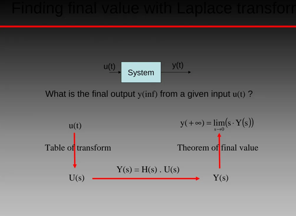
9/23/2009 III. Laplace transforms 46
System
u(t) y(t)
What is the final output y(inf) from a given input u(t) ?
u(t)
Table of transform
U(s)
Y(s) = H(s) . U(s)
Y(s)
Theorem of final value
( ) (
s Y s)
lim )
y(+ ∞ = s 0 ⋅
→
Finding final value with Laplace transform
9/23/2009 III. Laplace transforms 47
Poles and zeros
H(s) Y
U
Transfer function is a ratio of polynomials : ...
s a s a s a a
...
s b s b b
) s ( D
) s ( ) N s ( ) H s ( U
) s ( Y
3 3 2
2 1
0
2 2 1
0
+ +
+ +
+ +
= +
=
=
Poles and zeros :
( ) ( )
(
−) (
−⋅ −⋅ −) (
⋅ −⋅ ⋅⋅)
⋅ ⋅⋅⋅
=
=
3 2
1
2 1
0 0
p s p
s p s
z s z s a
) b s ( ) H s ( U
) s ( Y
zero : z1, z2, …
poles : p1, p2, p3…
p2
p1 z1
Re Im
p3
z2
• Poles and zeros are either into the left plane ore into the right plane
• Complex poles and zeros have a conjugate
9/23/2009 III. Laplace transforms 48
• Poles are the roots of Transfer function denominator
– Real values or conjugate complex pairs
• Poles are also the eigenvalues of matrix A
• Poles = modes
9/23/2009 III. Laplace transforms 49
Poles and zeros : decomposition
H(s) Y
U
Transfer function can be expansed into a sum of elementary terms : ...
s a s
a s a a
...
s b s b ) b
s ( ) H s ( U
) s ( Y
3 3 2 2 1
0
2 2 1
0
+ +
+ +
+ +
= +
=
p ...
s p
s p ) s
s ( ) H s ( U
) s ( Y
3 3 2
2 1
1 +
− + α
− + α
−
= α
=
p1 and p2 are conjugate : = −ω ⋅ ⋅θ = −ω0 ⋅ −j⋅θ j
0
1 e ,p2 e
p
p ...
s s cos 2
) s s ( ) H s ( U
) s ( Y
3 3 2
0 0
2
2 ,
1 +
− + α ω +
⋅ θ
⋅ ω
⋅ +
= α
=
First orders Second orders
☺ Complex system response is the sum of first order and second order systems responses
9/23/2009 III. Laplace transforms 50
Dynamic response of first order systems
U Y
p1
s ) 1 s (
H = +
( )
U( )
sp s s 1 Y
+ 1
=
Example 1 : impulse response
u(t) is an impulsion (0 everywhere, except in 0 : ∞)
u(t)
Table of transform
U(s)=1
Table of transform
( )
s H( ) ( )
s U sY = ⋅
( )
p1
s s 1
Y = +
t p1
e ) t (
y = − ⋅
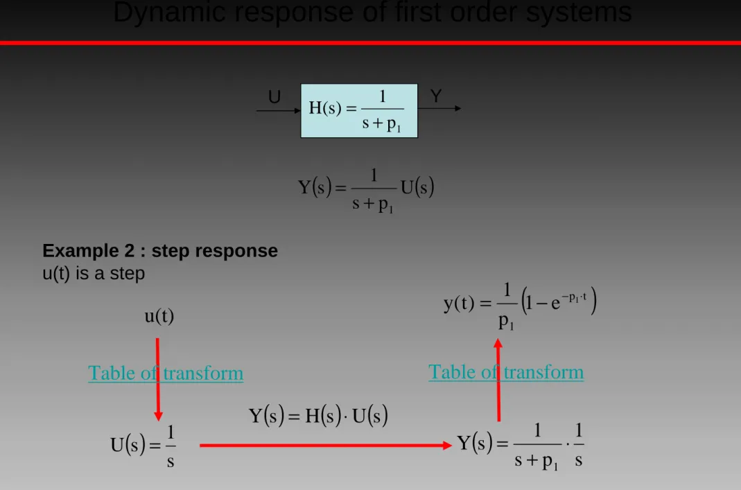
9/23/2009 III. Laplace transforms 51
Dynamic response of first order systems
U Y
p1
s ) 1 s (
H = +
( )
U( )
sp s s 1 Y
+ 1
=
Example 2 : step response u(t) is a step
u(t)
Table of transform Table of transform
( )
s H( ) ( )
s U sY = ⋅
( )
s1 p s s 1 Y
1
+ ⋅
=
(
p t)
1
e 1
p 1 ) 1 t (
y = − − ⋅
( )
s s 1 U =9/23/2009 III. Laplace transforms 52
Properties of first order systems
U Y
p1
s ) 1 s (
H = +
Step response
t1 = 1/p1 is the time constant of the system :
after t = t1, 63% of the final value is obtained
( )
U( )
sp s s 1 Y
+ 1
=
9/23/2009 III. Laplace transforms 53
2 0 0
2 2 s
s ) 1 s (
H = + ⋅σ⋅ω ⋅ + ω
Dynamic response of second order systems
U Y
Example 1 : impulse response
u(t) is an impulsion (0 everywhere, except in 0 : ∞)
u(t)
Table of transform
U(s)=1
Table of transform
( )
s H( ) ( )
s U sY = ⋅
(
1 t)
sin e
1 ) 1
t (
y t 0 2
2 0
à ⋅ ω −σ ⋅
σ ⋅
−
= ω −σ⋅ω ⋅
2 0 0
2 2 s
s ) 1 s (
Y = + ⋅σ⋅ω ⋅ + ω
9/23/2009 III. Laplace transforms 54
2 0 0
2 2 s
s ) 1 s (
H = + ⋅σ⋅ω ⋅ + ω
Dynamic response of second order systems
U Y
Example 2 : step response u(t) is an step
u(t)
Table of transform
U(s)=1/s
Table of transform
( )
s H( ) ( )
s U sY = ⋅
(
ω −σ ⋅ +( )
σ)
⋅ σ ⋅
−
− ω
= e−σ⋅ω ⋅ sin 1 t arcos 1
1 1 ) t (
y t 0 2
2 0
à
s 1 s
2 s
) 1 s (
Y 2
0 0
2 ⋅
ω +
⋅ ω
⋅ σ
⋅
= +
9/23/2009 III. Laplace transforms 55
Properties of second order systems
Step response :
σ is the damping factor ω0 is the natural frequency
2 0 0
2 2 s
s ) 1 s (
H = + ⋅σ⋅ω ⋅ + ω Y U
(
ω −σ ⋅ +( )
σ)
⋅ σ ⋅
−
− ω
= e−σ⋅ω ⋅ sin 1 t arcos 1
1 1 ) t (
y t 0 2
2 0
à
2 0 1−σ
ω is the pseudo-frequency 5% of the final value is obtained after :
0
% 5
t 3
ω
⋅
≈ σ
overshoot
Overshoot increases as σ decreases
9/23/2009 III. Laplace transforms 56
Properties of second order systems
Step response (continued) :
2 0 0
2 2 s
s ) 1 s (
H = + ⋅σ⋅ω ⋅ + ω Y U
poles : p1,2 = −ω0 ⋅e±θ cos(θ)=σ
θ ω0
Re Im
9/23/2009 III. Laplace transforms 57
Stability
Re Im
Unstable
Stable
unstable pole, deverges like exp(t)
stable pole, decays like exp(-4.t)
Any pole with positive real part is unstable
Any input (even small) will lead to instability
See animation
9/23/2009 III. Laplace transforms 58
« fast poles » vs « slow poles »
Re Im
slow
fast
slow pole, decays like exp(-t)
constant time : t1 = 1s fast pole, decays like
exp(-4.t)
constant time : t1 = 4s Fast poles can be neglected
See animation
9/23/2009 III. Laplace transforms 59
Effect of zeros
See animation
Re Im
Zeros modify the transient response
• Fast zero : neglected
• Slow zero : transient response affected
• Positive zero : non minimal phase system, step response start out in the wrong
direction
9/23/2009 III. Laplace transforms 60
Ex. analysis of a feedback system
Process model :
( )
+0.02⋅v = u −10⋅θdt t dv
Transfer function
s
:( ) ( ) ( )
( ) ( ) ( )
θ
⋅
−
=
⋅ +
⋅
=
⋅ +
⋅
s 10
s V 02 . 0 s
V s
s U s
V 02 . 0 s
V s
( ) ( ) ( ) ( ) ( )
− + θ =
= +
=
⇒
s 02 . 0
10 s
s V
s 02 . 0 s 1
s F U
s V
9/23/2009 III. Laplace transforms 61
Ex. analysis of a feedback system
Transfer function of the controller (PID) :
( ) ( ) ( ) ( )
( ) ( )
t k k s k 1sE t U
d t e dt k
t k de
t e k t
u
i d
t i 0 d
⋅ +
⋅ +
⇒ =
τ
⋅
⋅ +
⋅ +
⋅
=
∫
9/23/2009 III. Laplace transforms 62
Ex. analysis of a feedback system
We can now combine transfer functions :
vr -
F
θ
PID v
u
e -10
( )
s 1 F( )
s 1PID( ) ( )
s V s 1 F( )
s 10PID( ) ( )
s E sV r ⋅
⋅ +
+ −
⋅ ⋅
= +
9/23/2009 IV. Design of simple feedbacks 63
IV. Design of simple feedback
9/23/2009 IV. Design of simple feedbacks 64
P(s)
u y
Introduction
Standard problems are often first orders or second orders
• Standard problem standard solution
C(s)
d r
-
( )
s a s bP = +
( )
2 1
2
2 1
a s a s
b s s b
P + ⋅ +
= +
9/23/2009 IV. Design of simple feedbacks 65
Control of a first order system
Most physical problems can be modeled as first order systems
( )
s a s bP = +
Step 1 : transform your problem in a first order problem :
( )
sk k s
C = + i Step 2 : choose a PI controller
Step 3 : combine equations and tune k and in kiin order to achieve the desired closed loop behavior (mass-spring damper analogy)
( ) ( ) ( ) ( ) ( )
2 0
2 0
i i
s s 1 2
s ' b K 1
s k k
a s 1 b
s k k
a s
b s
C s P 1
s C s s P
CL
+ ω ω ⋅
σ + ⋅
⋅
⋅ +
=
+ + ⋅
+
+ + ⋅
⋅ = +
= ⋅
9/23/2009 IV. Design of simple feedbacks 66
2 0 0
2 2 s
s ) 1 s (
H = + ⋅σ⋅ω ⋅ + ω
Dynamic response of second order systems
U Y
Example 1 : impulse response
u(t) is an impulsion (0 everywhere, except in 0 : ∞)
u(t)
Table of transform
U(s)=1
Table of transform
( )
s H( ) ( )
s U sY = ⋅
(
1 t)
sin e
1 ) 1
t (
y t 0 2
2 0
à ⋅ ω −σ ⋅
σ ⋅
−
= ω −σ⋅ω ⋅
2 0 0
2 2 s
s ) 1 s (
Y = + ⋅σ⋅ω ⋅ + ω
9/23/2009 IV. Design of simple feedbacks 67
2 0 0
2 2 s
s ) 1 s (
H = + ⋅σ⋅ω ⋅ + ω
Dynamic response of second order systems
U Y
Example 2 : step response u(t) is an step
u(t)
U(s)=1/s
Table of transform
( )
s H( ) ( )
s U sY = ⋅
(
ω −σ ⋅ +( )
σ)
⋅ σ ⋅
−
− ω
= e−σ⋅ω ⋅ sin 1 t arcos 1
1 1 ) t (
y t 0 2
2 0
à
s 1 s
2 s
) 1 s (
Y 2
0 0
2 ⋅
ω +
⋅ ω
⋅ σ
⋅
= + Table of transform
9/23/2009 IV. Design of simple feedbacks 68
Properties of second order systems
Step response :
σ is the damping factor ω0 is the natural frequency
2 0 0
2 2 s
s ) 1 s (
H = + ⋅σ⋅ω ⋅ + ω Y U
(
ω −σ ⋅ +( )
σ)
⋅ σ ⋅
−
− ω
= e−σ⋅ω ⋅ sin 1 t arcos 1
1 1 ) t (
y t 0 2
2 0
à
2
0 1−σ
ω is the pseudo-frequency 5% of the final value is obtained after :
0
% 5
t 3
ω
⋅
≈ σ
overshoot
Overshoot increases as σ decreases
9/23/2009 IV. Design of simple feedbacks 69
Properties of second order systems
Step response (continued) :
2 0 0
2 2 s
s ) 1 s (
H = + ⋅σ⋅ω ⋅ + ω Y U
poles : p1,2 = −ω0 ⋅e±θ cos(θ)=σ
θ ω0
Re Im
9/23/2009 IV. Design of simple feedbacks 70
Control of a second order system
Step 1 , step 2 : idem (PI controller)
Step 3 : Transfer function is now third order
( ) ( ) ( )
( ) ( ) ( )
+ ω ω ⋅
σ + ⋅
⋅ +
⋅
⋅ +
⋅ = +
= ⋅
2 0
2 0
s s 1 2
s a 1
s ' b K 1
s C s P 1
s C s s P
CL
2 dof (k and ki) : the full dynamics (order 3) cannot be totally chosen
9/23/2009 IV. Design of simple feedbacks 71
Simulation tools
Matlab or Scilab
Transfer function is a Matlab object
Adapted to transfer function algebra (addition, multiplication…) Simulation, time domain analysis
9/23/2009 VI. Design of simple feedbacks (Ctd) 72
Conclusion
Laplace Transform +
Simulation tools
Design of simple feedbacks
9/23/2009 V. Frequency response 73
V. Frequency response
9/23/2009 V. Frequency response 74
Introduction
Frequency response :
• One way to view dynamics
• Heritage of electrical engineering (Bode)
• Fits well block diagrams
• Deals with systems having large order
– electronic feedback amplifier have order 50-100 !
• input output dynamics, black box models, external description
• Adapted to experimental determination of dynamics
9/23/2009 V. Frequency response 75
The idea of black box
The system is a black box : forget about the internal details and focus only on the input-output behavior
Frequency response makes a “giant table” of possible inputs-outputs pairs
Test entries are enough to fully describe LTI systems ☺
- Step response - Impulse response - sinusoids
System
u y
9/23/2009 V. Frequency response 76
What is a LTI system
A Linear Time Invariant System is :
• Linear
If (u1,y1) and (u2,y2) are input-output pairs then (a.u1+ b.u2 , a.y1+ b.y2) is an input-output pair : Theorem of superposition
• Time Invariant
(u1(t),y1(t)) is an input-output pair then (u1(t-T),y1(t-T)) is an input- output pair
The “giant table” is drastically simplified :
( ) ( ) ( ) ( ) ( )
s H s U sY
dτ u τ
t τ h y(t)
⋅
⇒ =
⋅
⋅
−
=
∫
−+∞∞9/23/2009 V. Frequency response 77