Adoption of technologies with network effects : an empirical examination of the adoption of automated teller machines

Digitized

by

the

Internet

Archive

in

2011

with

funding

from

Boston

Library

Consortium

Member

Libraries

•&&m

(!

7

ADOPTION OF TECHNOLOGIES UITH NETWORK

EFFECTS:

An

Empirical Examination

of the

Adoption of Automated Teller Machines

Garth Saloner

and

Andrea Shepard

No. 577

April 1991

massachusetts

institute

of

technology

50 memorial

drive

Cambridge,

mass.

02139

ADOPTION

OF

TECHNOLOGIES

WITH

NETWORK

EFFECTS:

An Empirical

Examination

of the

Adoption of Automated Teller Machines

Garth Saloner

and

Andrea Shepard

JUL

1 8 1991 RfeO.*

ADOPTION

OF

TECHNOLOGIES

WITH

NETWORK

EFFECTS:

An

Empirical

Examination

of

the

Adoption

of

Automated

Teller

Machines*

Garth

Saloner

Stanford University

and

Andrea

Shepard

Massachusetts

Institute of

Technology

Current Version: April 9, 1991

ABSTRACT

The

literature

on

networks

suggests that thevalue ofa

network

is positively affected

by

the

number

ofgeographically dispersed locations it serves (the

"network

effect")

and

the

number

ofitsusers (the "production scale effect").

We

show

that as aresult

a firm's

expected time

until

adoption

of technologies

with

network

effects declines

in

both

users

and

locations.

We

provide empirical evidence

on

the

adoption

of

automated

teller

machines by banks

that is consistent

with

this prediction.

Using

standard

duration models,

we

find that a bank's date of

adoption

is decreasing in

the

number

ofits

branches

(a

proxy

for the

number

of locations

and

hence

for the

network

effect)

and

the value ofits deposits (a

proxy

for

number

ofusers

and

hence

for

production

scale economies).

The

network

effect is the larger ofthe

two

effects.

*

We

_would

_{like to}

_thank

_Timothy

_Hannan

_and

_John

_McDowell

_{for generously}

allowing us to use their data,

Stephen

Rhoades

and

Lynn

Flynn

at the

Board

of

Governors

for providing Federal Reserve data,

Keith

Head

and

Christopher

Snyder

for research assistance,

Robert Gibbons,

Nancy

Rose,

and

Julio

Rotemberg

for

several helpful discussions,

workshop

participants at

Harvard

and

the

NBER

for

useful

comments,

the National Science

Foundation (Grant

IST-8510162), the

Sloan

Foundation,

and

the

Telecommunication

Business

and Economics

Program

at

MIT

forfinancial support.

1.

Introduction

With

the proliferation of information technology over the past several decades,

net-works have

become

increasingly important.

Examples

include banks'

automated

teller machines, airlines'

customer

reservation systems,

and

the

growing

network

of facsimile machines. In such networks, the value to each individual orfirm of

partic-ipating increases

with

network

size.

Network

effects,

and

demand-side economies

of scale

more

generally,

have been

shown

in theory to

have

implications for a variety of

important

economic

activities including technology adoption, predatory pricing,

and

product

preannouncements.

1

There have

not, however,

been

any attempts

to

test econometrically for the effects of

networks

on

these

phenomena.

2

In this

pa-per

we

construct

and

apply a test for

network

effects

on

the

adoption

by banks

of

automated

teller

machines

(ATMs).

For telephone systems,

which

are

perhaps

the best

known

example

ofa

technol-ogy with important network

effects, there are

two

types ofeffects. First, the benefit of the technology to

an

individual user increases in the

number

of telephones, i.e.,

in the

number

oflocations

from which

the

system can be

accessed.

This

size effect

also exists, for

example,

in retail distribution

networks

where

consumer

benefit

in-creases in the

number

of outlets at

which

the

good

is available. Second, the benefit increases in the

number

of people

who

are

on

the system: as the

number

of people

who

make

and

receive calls increases, each individual

can

communicate

with

more

people.

This second

effect is the source of

network

externalities

because

each

new

user confers

a

benefit

on

all other users.

In the case of

ATMs

the

network

effect is of the first type.

A

cardholder is

better off the larger the

number

ofgeographically dispersed

ATMs

from

which

she

can

access her account.

The

convenience of access to one's account

wherever one

happens

to

be

means

that the value of the

ATM

network

increases in the

number

of

ATM

locations it includes.

A

bank

can

increase its

network

size

by

adding

more

ATMs

to its proprietary

system

and

by

linking its

network with

the

networks

of

1

See, for

example,

Katz and

Shapiro (1986)

and

Farrell

and

Saloner (1985,1986).

2

Several case studies

have

been conducted

to confirm the relevance of the the-ories.

For example,

David

(1985) argues that

demand-side economies

explain the

other banks. In the early days of

ATM

adoption studied here, interbank

networks

were

quite rare for a variety of technical

and

institutional reasons.

As

a result the value of the

network

to depositors

was

increasing in the

number

of

ATM

locations

in their bank's network.

Because

differences in banks' post-adoption

network

size

would

generate

dif-ferent valuations to their depositors, the value of

adopting

an

ATM

system

would

be

higher for

banks

expecting to

have

larger proprietary

networks

in equilibrium,

all else equal.

Because

new

technologies diffuse gradually

through

an

industry, it

is

common

and

reasonable to expect those firms that value the technology

more

to

adopt

earlier. Ifeither thecost ofadopting

an

ATM

network

ofa given size fallsover

time

(because

banks and/or

suppliers

have

alearningcurve) or the benefit rises over

time

(because depositors learn

about

the value of

ATMs

or

ATMs

perform

more

functions),

then

banks with

a relatively higher valuation of the technology at

any

point in

time

will

adopt

relatively early.

A

reasonable version ofthe

network

effects hypothesis, therefore, is that

banks

expecting to

have

a larger

number

of locations in equilibrium will

adopt

sooner.

To

test this hypothesis

we

proxy

unobservable

expected

network

size

by

the

number

of

branches

a

bank

has.

Branches

are a

good

proxy

for

expected network

size

because

they

are the

most

common

location for

ATMs,

they are the lowest-cost locations,

and

because

legal restrictions limited

placement

outside

branches

during the

sample

period. Further,

commentary

in the trade press

and

casual

empiricism

suggest that

banks

eventually place

ATMS

in most, if not all, branches.

Accordingly

we

focus

on

the likelihood that

banks adopt

as a function of the

number

of

branches

they

have.

The

net value of

an

ATM

system

to a

bank

also will

be

affected

by

the

number

of its depositors to

whom

ATMs

are valuable.

Because

there are fixed costs of

adoption,

economies

of scale in production

mean

that a bank's propensity to

adopt

will increase in the

number

of these depositors. Indeed, earlier studies of

ATM

adoption

by

Hannan

and McDowell

(1984, 1987) find that

bank

size, as

measured

by

total assets, is

an important determinant

of

time

of adoption.

We

confirm

these results

by

including a

measure

of size

more

directly related to the

number

of

we

are able to separate the

network

effect

from

the scale

economies

effect.

Controlling for variation in the

number

of depositors

and

other heterogeneity,

we

find that increasing

network

size increases the probability of early adoption.

When

evaluated at the

sample

mean,

the estimated probability that a

bank would

have adopted

in the first nine years

ATMs

were

available is 17.1 percent.

Adding

a single

branch

increases this probability

by

at least 5.7 percent (to 18.1 percent)

and

perhaps

by

as

much

as 10 percent. In comparison,

adding

enough

depositors

to equal

an

average sized

branch

increases the adoption probability

by

4.3 percent.

The

strong

network

effect is robust to specification

and

to

removing

large outliers.

In section 2,

we

discuss the determinants of

ATM

adoption

and

develop a test for

network

effects. In Section 3

we

briefly discuss the statistical

models

used.

The

data used

to

implement

these

models

are discussed in Section 4,

and

in Section 5

we

present

our

results. Section 6 provides

some

concluding

comments.

2.

Network

Effects

and

ATM

Adoption

In this section

we

develop a

framework

for considering a bank's

adoption

decision.

While

thisdiscussion does not identifystructuralparameters, it does provideinsight into the relationship

between network

size

and

a bank's propensity to

adopt

ATMs

that guides the empirical analysis. In particular,

we

focus

on

distinguishing the

effect of

network

size

from

the effect ofthe

number

ofend-users.

In our context, end-users are the bank's depositors

and

the relevant

measure

of

network

size is the

number

of physical locations at

which any

given depositor

can

carry out

a

transaction.

While

each user is largely unaffected

by

the

number

of

other users of the

same

network, each user is better off the greater the

number

of outlets

from

which

she

can

access the network. Feasible locations for

ATMs

include the bank's

branches

and

may

also include

some

non-branch

locations.3

To

simplify

theanalysis

and

be

consistent with the

data

availableforempirical work,

we

assume

that if a

bank

decides to

adopt

ATMs

it will

be

optimal for it to install

ATMs

in

all feasible locations

and

make

the

system

accessible to all its depositors.

3

As

discussedin asubsequent section,placing

ATMs

outsideof existing

branches

We

start

with

banks

endowed

with a set of characteristics including its

depos-itors

and

feasible

ATM

locations.

Throughout

the analysis,

we

treat these

charac-teristics as predetermined, focusing

on

the adoption decision conditional

on

bank

characteristics.

With

the

number

of depositors

and

potential

network

size prede-termined, a

bank

decides

whether

to

adopt

an

ATM

system

ofa fixed size to serve

a fixed

number

of depositors and, if so,

when.

The

bank's decision,

depends

on

the flow of benefits

and

costs

from

adoption.

We

begin

by

considering the "benefit side",

and

in particular, the benefits to

an

individual user. In the theoretical literature

on network

effects,

an

end-user's per period benefits are frequently represented

by

a

+

b(N),

where

a represents the "stand-alone" benefit

from

the technology

and

b(N)

represents the

network

effect.4

The

"stand-alone" or

"network

independent"

component

ofthe user's benefit is that

which

the user obtains regardless ofthe sizeofthe network.

Thus,

a

might

represent

the utilitythat a depositor receives

from

having

an

ATM

installed at the

branch

she

"usually" uses: the depositor

may

get superior service simply

by

substituting the

automated

teller for the

human

one

during

normal

business hours,

and

will

be

able to lengthen the period during

which

she

can

transact at that

branch

by

substituting

an

after-hours

ATM

for a

daytime

teller.

The

network

effect term, b(N), increases in

N

which measures

the size of the

network

(JV

>

1).

The

variable

N

then represents the

number

of other locations

from

which

a depositoris able to accessher account

from

an

ATM.

Ifthose

ATMs

are

located at existing

branches

the benefits they provide are of

two

kinds. First, they provide the benefits discussed

above

of substituting

machines

for tellers

and

after-hours

use for

daytime

use. Second,

by

standardizing depositor identification

and

account

access procedures the existence of

an

ATM

in

branches

other

than

the

one

at

which

the user has

an

account

may

make

it easier for the userto transact at those branches. Ifthe

ATMs

are not locatedat existingbranches, theyeffectively increase

the

number

of

branches

(for the subset oftransactions that

can

be performed by an

ATM).

5

4

See Farrell

and

Saloner (1986) for example.

5

In this setting a

probably

depends

on

N.

The

valueof

having

an

ATM

at one's

The

aggregate per period value of the

ATM

network

to a bank's depositors if

there are

n

of

them

is n[a

+

b(N)]. In general

one

might

expect the per period

benefits to increase with calendar time as the

number

of services

which

ATMs

provide increase. In

what

follows

we

suppose

that benefits

have

growth

factor g,

where

g

>

1.

The

flow of benefits that the bank's users derive

from an

ATM

during

period t is therefore [a

+

^N^g*.

Assuming

that the per-period increasein revenues

to the

bank

is proportionalto theper-period benefitsto the depositors (inparticular if the bank's revenues are A times the benefit to depositors

where

A

<

1),

then

the

present value of the bank's revenues (evaluated at time

T) from adopting an

ATM

at

time

T

are:

oo

J]An[a

+

6(iV)]^

T+t (1)

<=o

where

8 is the discount factor.

Note

that these benefits are increasing in

both n

and

N.

6

We

turn

now

to the "cost" side ofthe analysis. In

making

its

adoption

decision,

the

bank must

consider

both

variable

and

fixed costs.

The

variable costs are

mainly

supplies (such as film) that are incurred with each transaction.

Because

we

assume

that each depositor

makes

the

same

number

of transactions, the variable costs are proportional to the

number

of depositors. For simplicity,

we assume

that the

variable costs are incorporated in A so that \n[a

+

b(N)]gl

represents the benefit

net of variable cost in period < to a

bank

that has

adopted

an

ATM.

The

fixed costs include the cost of

making

alterations to

branches

to

accom-modate

ATMs,

expenses related to adapting the bank's

computer

software to the

ATMs,

the cost of purchasing or leasing the

ATMs

themselves, the cost of service to

maintain

the distinction

between

stand-alone effects

and

the

network

effect of

additional locations in

what

follows. For simplicity

we

suppress the

dependence

of

a

on

N

in the notation. If this effect is

important

it will reduce the

network

effect

measured

in the empirical work.

6 _{For reasons discussed}

at length later (principally that

banks

did not share

ATM

networks

in the 1970s),

we

assume

that

bank

A's depositors are

unable

to use

bank

B's

ATMs.

Therefore

N

represents only the bank's

own

ATM

locations. If

such networks were

shared

and

if a

bank

thereby obtained

some

benefits

from

the

adoption

of

ATMs

by

other banks, there

might

be

an

externality in banks'

adoption

decisions. In

our

case,

where

each bank's

network

benefits are

independent

ofother banks' actions,

no

externality is involved.

Hence

the

term "network

effect".

and

the cost of marketing.

Many

of these costs, such as the cost of

purchasing

or leasing

ATMs

or of installing

them,

depend

on

N.

Others, such as software or

marketing

costs, are

"system

costs"

and

are arguably

independent

of

N.

We

de-note the present value of the cost of adopting

an

ATM

system

in

N

locations at

time

T

as

C(N,T)

=

S(T)

+

JVc(T),

where S(T)

represents the

system

costs

and

c(T) represents the cost per location.

A

typical

assumption

in the literature

on

the

adoption

of technology,

and

one which

we

make

as well, is that the fixed cost of

adopting

the technology,

C(N,T),

declines over

time

as the suppliers'

and/or

the banks' experience

with

the technology accumulates.

The

net present value of

a

bank's profits

from adopting

ATMs

at time

T

is therefore:

oo

II

=

^

A«[a

₊

b(N)]6t_gT+t

-

C(N,

T).

<=o

A

bank

with

n

depositors

and

N

locations earns higher profits

from adopting

at

time

T

than

from

waiting until time

T +

1 if:

A*

T

f

+

«*>'

-C(N,T)

>

if**'*

1

*?

KN)]

-

C(N,T

+

1)), 1

—

og V 1

—

Og t

Anto

+

W-^,,^

1

-

og i.e., if Xn[a

+

b(N)]g

T

> C(N,T) - 6C(N,T

+

1). (2)

The

assumptions

that variable profits

grow and

the cost of

adoption

declines over

time

implies that every

bank

eventually finds it profitable to

adopt

ATMs.

This

allows us to focus

on

when,

rather

than

whether,

adoption

takes place.

Provided

the rate of decline of the cost of

adopting

decreases over time, the smallest

T

that

satisfies

Equation

(2) is the optimal time to adopt.7

There

are

two

interesting polar cases of

Equation

(2).

The

first is

where

C(N,

T)

is constant over

time

so that

growth

is the only factor in the

timing

of

adoption. In that case

Equation

(2) reduces to:

Xn[a

+

b(N)]g

T

1-8

>

C(N),

7

A

similar

model

of the optimal

adoption

time (but

without

network

effects) is

i.e., the

bank

adopts as

soon

as the net present value of variable profits

assuming

no

further

growth

exceeds the cost ofadoption. Since costs

do

not decline

with time

in this case there is

no

point to waiting: future per-period profits will

be

higher

than

today's,

and

if

adoption

would be

profitable with a

stream

of profits equal to this

period's, the

bank

should adopt.

The

second

polarcaseis

where

thereis

no growth

_(g

=

1)

and

theonly

temporal

effect is the declining cost of adoption over time.

Then

Equation

(2)

becomes

\n[a

+

b(N)]

> C(N,T) - SC(N,T

+

1).

The

right-hand-side ofthis expression is

the cost-saving

from

delaying adoption

by one

period,

and

the

bank

adopts

as

soon

as that cost saving is less

than

the (constant) per-period variable profit.

The

general case

(Equation

(2)) is a

combination

of these

two

effects.

The

bank

adopts

when

the per-period variable profits exceed the cost-saving ofwaiting

an

additional period.

Each

period adoption

becomes

more

tempting both because

per-period variable profits are higher

and

because the cost of

adoption

is lower. In this

model

n

enters

on

the left-hand-side of (2) only, i.e., it increases the

benefits (net of variable costs)

and

does not affect fixed costs.

As

is

apparent

by

dividing (2)

by

n, the bank's net benefit per depositor is constant, but total costs

decline in n; there are production side

economies

of scale in

ATM

systems.

As

a

result of these scale economies, the bank's profit

from an

ATM

system

is increasing in n. Therefore,

adoption

occurs earlier the larger the

number

of depositors.

In the empirical work,

we

are interested primarily in testing for a

network

effect

and

assessing its

magnitude.

This requires separating the effect of variation

in

network

size

from

the effect ofvariation in

number

ofdepositors.

One

simple test

for

network

effects is to estimate the effect of variation in

N

holding

n

constant.

However

correctly interpreting the result is complicated

by

the cost-side effects.

The

overall effect of

N

on

the timing of adoption is

ambiguous

since it affects

both

the left-

and

right-hand-sides of (2).

The

left-hand-side of (2) is increasing

in

N

because

of the

network

effect.

However,

the right-hand-side also increases

8

_The

assumption

that fixed costs are not

a

function of

n

is violatedif

usage

levels

vary across locations, particularly if

banks respond

to usage variation

by

varying

the

number

of

ATMs

across locations. Multiple

ATMs

per location

was

perhaps

less

common

in the early days of

ATM

adoption studied here

than

it is

now.

Iffixed costs increase in n, the sign of the overall effect of

n

is, in principle,

ambiguous.

with

N.

To

see this recall that

C(N,T)

=

S(T)

+

Nc(T),

so that the

right-hand-side of (2) is [S(T)

-

S(T

+

_1)]

+

N[c(T)

-

c(T

+

1)].

Two

banks with

different

numbers

of locations enjoy the

same

benefits in terms of reduction in the

system

costs if they wait;

however

the

bank

with

more

locations reaps the reduction in

the location specific costs at

more

locations.

Thus,

holding

n

constant,

banks with

more

locations will

adopt

earlieronly ifthe

network

effect

outweighs

this cost effect.

Consequently a

test that

measures

the effect of

N

on adoption

propensities, holding

n

constant, is

immune

to false positives, but will tend to understate the

network

effect

and

may

yield a false negative.

An

alternative

way

to get at the

network

effect is to hold

n/N

=

v constant

rather

than

n, that is, to hold constant the

number

of depositors per location

and

increase the

number

of locations. Dividing (2)

by

n

gives:

M

„

+

KN)] >

md-^+di

+

[cm-^T+i^

n

v

Holding

v constant

removes

the

downward

bias

from

the additional location-specific

cost.

However, because

increasing

N

while holding v constant

adds

both a

location

and

v depositors to the network,

an

upward

bias is introduced.

The

term

involving

S

is

now

decreasing in

n

because

system

costs are spread over

more

depositors.

Thus

if

banks with

more

locations (holding v constant) are

found

to

have

a higher propensityto

adopt

this couldsimply

be

due

to increasingreturns to scale in

system

costs

and

not

due

to the

network

effect. This test, then, will overstate the

network

effect

and

can

yield false positives but not false negatives.

In

summary,

examining

the propensity to

adopt

holding

n

constant understates the

impact

of the

network

effect, while holding

n/N

constant overstates it.

As

described in Section 5,

we

test for the presence of

a network

effect

by

holding

n

constant,

then

use these

two

assessments to

bound

the

magnitude

of the

impact

of

the

network

effect.

The

size of the

network

effect will

be

closer to the

upper

bound

estimate if location-specific costs are

more

important

than

system

costs.

We

have

assumed

thus far that thereis

no

variationin the valuationof

an

ATM

network

among

banks with

the

same

number

of depositors

and

ATM

locations. In practice, however, this is unlikely to

be

the case. For

example,

some

banks might

Alternatively, the benefits of after-hour

banking might be

greater for

some

banks,

such

as those situated in the suburbs,

than

for others. In this case,

among

the

banks

with a given

number

of depositors

and

locations, the

banks

for

whom

such

idiosyncratic benefits are the greatest will

adopt

earliest while the others wait.

To

take account of such differences

among

banks, let et

- (E(ei)

—

₀₎ represent

the deviation of the per period profits of

bank

i

from

the

mean

profit of

banks with

the

same

number

of depositors

and

locations. In this case the net present value of

a

bank's profit

from adopting

at time

T

is:

and

Equation

(2)

becomes:

e,

>

C(N,

T)

-

SC(N,

T

+

1)

-

\n[a

+

b(N)]g

T

, (3) i.e.,

banks with

idiosyncratically large net benefits

adopt

early while others wait.

The

smallest

T

;

=

T(n,

N,

e;) that satisfies (3) is the optimal

adoption

date for the

ith bank.

In general the rate of adoption

may

change

over time.

This

depends on

how

the cost or benefits of adoption

change

over time

and

on

how

e; is distributed.

To

see this, use

Equation

(3) to define:

e*i(n,

N, T)

=

C{N,

T)

-

6C(N,

T +

1)

-

Xn[a

+

b(N)]g

T

. ₍₄₎

Then

e*(n,N,T)

is the e; of the

bank

with

n

depositor

and

N

locations that isjust

indifferent

between adopting

and

not adoptingat time T.

Then

theprobabilitythat a

bank

with

n

depositors

and

N

locations adopts in period

T

(i.e., the

hazard

rate

at period

T)

is:

H[e*(n,N,T

+

l)]-H[e*(n,N,T)}

l-H[e*(n,N,T)}

' l°J

where

H(-) is the cumulative distribution function for e. If, as

assumed

above, the benefits of

adopting

relative to costs increase over time, the right-hand-side

of equation (4) decreases with T. Therefore

even

if e is uniformly distributed so that the

numerator

of (5) is constant over time, the

denominator

declines in T.

As

a result,

more

banks

find it profitable to

adopt

each period

than

did the period

before.

Moreover,

if e, is

normally

distributed, say, then in the early periods

when

the

Normal

density is

an

increasing function

even

more

banks

find it profitable to

adopt each

period

than

the period before so that this

tendency

is reinforced. For

both

of these reasons

we

expect to find positive duration

dependence

in the

hazard

rate.

3.

Estimation

Models

Equation

(4) implies that

adoption

time, conditional

on

a bank's observable charac-teristics, is a

random

variable.

The

choice of

an

estimation

model

involves choosing

a

distribution for

adoption

dates. In addition,

because

our

observations of

adoption

times are right-censored, the estimation

model must

accommodate

censoring.

The

strategy

we

follow is to estimate

standard

duration models.

These

models

easily

incorporate censored observations

and

yield readily interpretable

reduced

form

pa-rameters.9

The

duration

model

which

is the

main

focus of

our

analysis

assumes

that the

time

until

adoption

for

bank

i conditional

on

its characteristics follows a

Weibull

distribution. Let Xi

be

the vector ofobserved characteristics for

bank

i

and

/?

be

the

unknown

coefficients.

Then

theprobability that

bank

i

adopts

before

time

T

is given by:

For

convenience,

we

make

the standard

assumption

that ip^x'^)

can

be

written as

An

attractive feature of the Weibull distribution is that the

computation

of

the effects of the covariates

on

adoption probabilities

from parameter

estimates is

relatively simple.

The

hazard

rate is (l/f)ip(x'

i(3)t

1~1/~t

.

Under

the

assumption

that ^(x'jP)

—

ex <P, the estimated coefficients are simply the effect of

x

on

the log

of the

hazard

rate.

The

Weibull distribution allows the

hazard

rate for a given

bank

to

change monotonically

over time. This probability increases, declines, or is

9

For a discussion of duration

models

in general, see Kiefer (1988),

and

for

an

overview

of applying these techniques to technology diffusion, see

Rose

and Joskow

(1990).

constant as

7

is less than, greater than, or equal to one.10

For

reasons discussed in

Section 2,

we

expect to find

7

<

1.

The

Weibull, however, constrains the

hazard

rate in

two

potentially

important

ways. First, it requires that duration

dependence be monotonic.

A

standard

em-pirical regularity in diffusionstudies is

an

initially increasing then declining

hazard

rate. Since

we

have data on

only the early years of the diffusion process for

ATMs,

it

seems

likely that a functional

form

that allows a monotonically increasing rate

will

be

adequate. Nonetheless, a

more

general functional

form

is a useful check

on

the

Weibull

results. Second, the Weibull (in

common

with

the other

members

of

the family of proportional

hazard models)

constrains the relative

hazard

rates of

any

two

banks

to

be

constant over time. For

example,

the ratio of the

hazard

rate

of a

bank

with

many

depositors

and

many

locations to the

hazard

rate of a

bank

with

many

depositors

and

one

location is

assumed

to

be

time invariant.

Suppose,

however, that the date ofadoption conditional

on

bank

characteristics is

Normally

distributed.

Then

this ratio

might be

relatively large early

on

and

decline over

time.

This

could

happen

because, with a

Normal

distribution, the density

func-tion of the

many-location

bank

can

be

declining while the density function for the

single-location

bank

is increasing.

To

test the results for sensitivity to the constraints

imposed

by

the Weibull,

we

estimate a duration

model

in

which

the underlying

adoption

date distribution

is

assumed

to

be

log-logistic.

The

log-logistic distribution allows a

non-monotonic

hazard

rate

and

allows relative

hazard

rates to

change

over time. It

approximates

a

model

in

which

the log of adoption dates is

Normally

distributed. For the log-logistic, the probability that

bank

i has

an

adoption date earlier

than

T

is given by:

1_

Ii

+

ti/7^(x;/?)J'

10

_The

_Weibull

is

a

generalization of the exponential distribution

used

in the

Hannan

and McDowell

(1984, 1987) analysis. It collapses to the exponential

when

7

=

1.

Although

they

assume

a time invariant underlying

hazard

rate,

Hannan

and

McDowell

use

time

varying covariates so that the

hazard

rate

can

change

as

bank

characteristics

change

over time.

We

have

chosen

an

alternative

approach

of

allowing the

hazard

rate to

be

a function of t directly

and

using each bank's 1971

characteristics.

With

this approach,

bank

characteristics are necessarily exogenous.

where

we

assume

again that i/>(x'

t(3)

=

exp(x[/3).

The

hazard

rate is

l

+

^lx'ipph

For

7

less

than

1, this functional

form

has

an

underlying

hazard

function that

initially increases

and

then decreases over time. If

₇

is greater

than

orequal to one,

the underlying

hazard

function has negative duration

dependence.

For

both

distributions, the likelihood function for observations

on

m

banks

is:

m

Y[f(x'

i

p,T,

7

)

d

<[l-F(x'

_i

p,T

n

)] 1

-

di

where

d

is

an

indicator variable equal to

one

ifthe firm adopts

and

/(•) (F(-)) is the density function (cumulative distribution function) for the

Weibull

or log-logistic

distribution.

The

first

term

is the contribution to the likelihood of a firm

observed

to

adopt

at

time

T; the

second

term

is the contribution of a firm failing to

adopt

prior to

time

T

after

which

it is

no

longer observed.

Both

these

models

assume

a distribution for

adoption

times conditional

on

bank

characteristics. If these parameterizations fit the

data

badly, the coefficient

estimates

may

be

adversely affected.

We

therefore

compare

these

parametric

es-timates to results

from

a

nonparametric (Cox)

partial-likelihood estimator.

This

estimator

makes

no assumption about

the underlyingdistribution of

adoption

times,

but

insteaduses the proportional

hazard

model

assumption

that the ratiosof

hazard

rates for

any two banks

are

time

invariant

and

estimates the relative probabilities.

4.

Data

Testing the hypothesis that

network

size

matters

given the

number

of depositors

requires variables that capture

network

size,

number

of depositors,

and

date of

adoption.

This

section describes these variables as well as variables

used

to control

for other

bank

characteristics that

might

affect

adoption

probabilities

and

be

cor-related

with

the variables ofinterest. Descriptive statistics for the variables

used

in

the analysis

appear

in

Table

1.

The

data

base includes information

on

adoption

dates,

bank

characteristics

and

state regulations.

Because adoption

is presumptively

more

likely in

urban

areas,

the

sample

was

restricted to

commercial banks

operating in a

county

that

was

part of

an

SMSA

or

had

a population center of at least 25,000 in 1972.

This

subset of all

commercial banks

in operation

between

1971

and

1979

was

further restricted to

conform

to the available

adoption

data

and

to capturevariationin

network

size.

The

final

sample

includes all

commercial

banks

that satisfied the geographic criterion in

1971

and

that existed

throughout

the 1971-1979

sample

period.

The

adoption data

come

from

surveys of all

commercial

banks conducted by

the Federal Deposit Insurance

Corporation

in 1976

and

1979.

The

1976

survey asks the year the

bank

first installed at least

one

ATM.

The

1979 survey asks

whether

the

bank

has installed

an

ATM

by

the 1979

sample

date.

Combining

these surveys

gives a date offirst

adoption

for

banks

adopting prior to

1977

and

identifies

banks

adopting between 1976

and

1979.

Year

of adoption for these later adopters

was

collected

by

a

supplementary

survey

conducted by

Hannan

and

McDowell

(1987).

n

The

date of

adoption

is the year the

bank

first installed at least

one

ATM.

Because

the surveys cover only

banks

existing at the survey dates, consistency requires that

our

sample be

restricted to

banks

existing in 1976

and

1979. Since

we

use 1971

characteristics data, the

sample

also is restricted to

banks

in existence

by

1971.

The

adoption data were

merged

with

data

on

firm characteristics

maintained

by

the Federal Reserve

Board

in the

Report

ofCondition

and Income and

the

Sum-mary

of Deposits.

These

sources

have

detailed balance sheet

and

other

summary

information

on

all

commercial

banks

operating in the

United

States. In particular,

they contain the best available information

on

number

of depositors

and

network

size as well as information

used

to control forother dimensions of

bank

heterogene-ity.

In the 1990s

ATMs

are

commonly

linked in regional

and

national networks. For at least

some

ATM

transactions then, the relevant

network

size is

now

the size

of the interbank network. In the 1970s, however, interbank connections

were

un-11

The

raw

survey

data

and

the

supplementary

information

on

lateradopters

were

generously given tous

by

Hannan

and

McDowell.

Our

sample

has

been

constructed

to

be

roughly consistent

with

theirs. Despite their efforts,

adoption

dates are not

available for

87 banks

known

to

have

adopted

and

otherwise consistent

with

the

sample

definition.

Except

where

otherwise noted, these

banks have

been

dropped

from

the sample.

common.

Many

of the early

machines were independent

units; they

were

not fully

connected with

the bank's

data

system, let alone

an

interbank system. Further,

in the early seventies

ATM

producers

had

not yet achieved a technological

stan-dard

that

would

make

machines

compatible. Legal issues

with

respect to shared

ATMs

also

slowed

the

development

of interbank networks. Interstate

banking

was

not

permitted

in this period

and

many

state's regulated the

number

and

location of

bank

branches.

Allowing

interbank

networks

would

clearly affect the existing

regulatory regimes,

and

sharing

was

delayed while regulators decided

how

it

should

be

managed.

State

and

federal rulings

on

interbank

networks

have

reflected

both

a concern

that large, single

bank

systems might

reinforce the

market

dominance

of

banks

already large

and

a countervailing concern that cooperative

arrangements

among

banks might

create collusive pricing.12

The

combination

ofpotential or

ac-tual legal constraints

and

the

rudimentary

state of the

new

technology

meant

that interbank

networks were

not

important

in the 1970s.

As

a result, the

network

size

relevant to a cardholder

was

the size ofher bank's proprietary network.13

For these single

bank

networks, the relevant

network

size is the

number

of

ATM

locations the firm

expected

to

have

in equilibrium

when

making

the

adoption

deci-sion.

This

number,

however, is inherently unobservable.

Even

if the

data

reported

the

number

of

ATM

locations for each

bank

in each year, these

numbers would

not

necessarily include the

planned

equilibrium

number.

14

We

therefore use the

number

of

branches

a

bank

has

(BRANCH)

as a

proxy

for

expected network

size.

BRANCH

12

For a review of the law

on

interbank networks, see Felgran (1984). 13

If

banks

anticipated that

ATM

networks

would

ultimately

be

interlinked, this

would

ofcourseaffect theirestimatesofthe net present value of benefits in

Equation

(1).

However, provided

that in the 1970s

banks

believed that

such

interlinking

would

not

occur

until the 1980s, such benefits

would

be

irrelevant to the

timing

of

adoption

decision represented

by Equation

(2).

However

the analysis in Section

2 ignores possible competitive

advantages

that

might

accrue to

banks

that

adopt

early.

For

example,

iffirms that pioneerinterbank

networks

are able to extract

some

of the rents

from

the creation of such networks,

and

if

banks with

many

branches

who

adopt

early are well-positionedin the competition to

form

interbank networks, those

banks

would

have

an

added

incentive to

adopt

early.

We

hope

to consider

such

competitive incentives to adopt,

which

are largely ignored in this paper, in

future work.

14

In fact, the

data

do

not report the

number

of

ATM

locations.

Nor

is the

number

of

ATMs

installed systematically available.

is

an

excellent

proxy

if

banks

typically place at least

one

ATM

in

each

branch

and

place relatively

few

or

no

ATMs

elsewhere.

Banks

tend to place

ATMs

in branches for several reasons. Installing

and

maintaining

ATMs

on

the premises of existing branches

may

be

less expensive

than

at off-premise locations.

Consumers

also

may

-at least in the early

days

of

ATM

use covered in this study -

have

felt

more

comfortable using

machines

located

where

they could get assistance with usage problems. Further, the legal status of

off-premise

placement

was

unresolved for a substantial portion of the

sample

period.

State regulatory agencies

and

legislatures control

whether

off-premise

placement

is allowed for state chartered banks. For national banks, off-premise

placement

is controlled

by

the

Comptroller

ofthe Currency. In 1979, the

Comptroller

ruled that

off-premise

placement by

national

banks

would be

allowed.15

Some

state authorities

acted to allow off-premise

placement

prior to the Federal ruling

and

some

tied state regulations to the Federal standard. Still others

had

not yet issued regulations for

off-premise

placement

by

1979.16 Until off-premise

placement

was

authorized, the

number

of

branches

was

aclear

upper

bound

on network

size.

Even

when

off-premise

placement

was

allowed, on-premise

placement

was

more

common.

Commentary

in

the trade press during this period suggests that

banks

eventually place

ATMs

in

most

branches

so that the

number

of branches is also a

good

lower

bound.

Because

states regulate branching, the distribution of branches per

bank

will

vary across states. In

some

states, branching is not allowed;

banks can have

no

more

than

a single

banking

office.

Because

there is

no

variation in

network

size in

these states,

banks

in these states are not included in the sample.17

As

a result,

the

2293

banks

in the

sample

are distributed over the 37 states in

which

multiple

branches

were

allowed in 1971.

Among

these states, 19 placed

no

restrictions

on

15

This

ruling

meant

that the Federal

government no

longer

had

an

interest in

regulating

ATMs.

As

a result, national

data

on

ATMs

were

not collected after 1979.

16

Most

states regulate off-premise

placement

in

some

fashion

even

where

it is allowed. For

example, banks

may

be

required to get approval for

each

off-premise location or to share off-premise locations

with

rival banks.

17

In principle, these single

branch

banks can be

included in the analysis to

pro-vide additional information

on

the effect of variation in the

number

of depositors

on

adoption

probabilities.

But

including

them

does not substantively affect the

parameter

estimates.

the

number

or location ofbranches.

We

refer to these states as "unrestricted".

The

remaining

18 states

had

some

limitation

on

the

number

or location of branches.

Banks

in these "limited" states

may

be

required to restrict

branching

to, say,

a

single

county

or to refrain

from

placing a

branch

in a small

community

already

served

by

a competitor.18

Ideally, the

n

in

Equation

(1)

would

be

implemented

as the

number

of

deposi-tors for

whom

ATM

transactions

have

value.

A

close

proxy

might

be

the

number

of

depositors

with

personal checking accounts.

However,

there are

no data

available

on

the

number

of accounts of

any

type.19

The

next best

proxy

is total deposits

by

customers

who

would

use

an

ATM.

This

proxy

might

be

affected

by

variation in the

size of accounts across banks.

The

closest available

proxy

is

"demand

deposits

by

individuals, partnerships,

and

corporations"

(DEPOSITS).

DEPOSITS

specifically

excludes

time

and

savings deposits (certificates of deposits

and

savings accounts,

for

example)

and

other less liquid holdings, as well as deposits held for other

banks

or the public sector, but includes

commercial

demand

accounts

even

though

these

accounts

probably

do

not generate

ATM

demand.

The

extent to

which

DEPOSITS

is a

good

proxy

for

n

depends

on

how much

variation there is in the proportion of

individual accounts in

DEPOSITS

across banks.

Four

additional variables are

used

tocontrol for other factors that

might

affect

adoption:

wage

in the area

(WAGE),

labor

expense

per

employee

(WB/L),

the average

number

of

branches

per

bank

in the state

(PROPBR),

and

product

mix

(PRODMDC).

The

wage

variable is included to control for variations in

ATM

value

arising

from

variations in labor cost. Iftellers are

more

expensive, technology that

can

substitute for tellers should

be

more

attractive. In this case, higher

wages

should

promote

ATM

adoption.

On

the other hand, the wage, as

a

measure

of

average

income

in the bank's area,

may

also

be

correlated

with

the average size 18

_The

_{data used}

to classify states with respect to

branching

regulations

were

provided

by

the

Conference

of State

Bank

Supervisors.

Two

states

changed from

limited to unrestricted regulation during the

sample

period.

Because

substantive

changes

in

branching

regulations

might change adoption

behavior, observations for

banks

in these states are treated as censored at the date of change.

19

_The

only

data

on

number

ofaccounts

come

from

the Functional

Cost

Analysis

reports.

These

data

are not publicly available in disaggregate

form

and

cover only

a

very small,

nonrandom

sample

of banks.

of checking accounts. If people with higher

income

typically hold larger

demand

deposits, the

WAGE

variable

may

pick

up some

variationinthe relationship

between

DEPOSITS

and

the

number

ofcustomers for

whom ATMs

are of value.

The

wage

used

is the average

manufacturing

wage

for 1977.20

The

bank's labor

expense

per

employee

is total expenditures

on

salaries

and

benefits divided

by

the

number

of employees.

There

is

some

evidence that this

variable is high in concentrated markets,

presumably because

of rent sharing

with

employees

(Rhoades

1980). In that case,

banks

with high values of

WB/L

may

be

more

likely to

adopt because

they

can

extract a larger share of the resulting

consumer

value (i.e., they

have

higher As in

Equation

(1)

than

banks

in less con-centrated markets).

On

the other hand,

WB/L

might

capture variation in the

mix

ofbanks' employees. It is possible, forexample, that a

bank

with

a relatively high value for

WB/L

has fewer relatively

low-wage

tellers

and

more

relatively

high-wage

commercial

account

managers

or investment advisors.

A

high valueof

WB/L

might

therefore indicate a low proportion of individual depositors and, therefore, a

low

propensity to adopt.

The

variable

PROPBR

is included to absorb variation in state

branching

reg-ulations.

Within

the limit category there is substantial variation in the severity of

the

branching

restrictions.

As

a result, the average

number

of

branches

per

bank

in limit states varies

from

less

than

2 to

more

than

8.21

Increasinglyrestrictivebranching regulationssuggest that thestand-alone value

of

adoption

(a in

Equation

(1))

might

be

higher.

The

reason for this is that a

depositor at a

bank

with, say, a single

branch

has

no

substitute for visiting that bank's single location during

normal

business hours.

By

contrast, a depositor at

a

multi-branch

bank

may

at least

be

able to substitute a transaction during

normal

20

As

reported in the City

and County

Data

Book.

21

Wisconsin

banks

average less

than

1.5. branches per bank,

and

branching

is

allowed only within the

same

county

as the bank's

main

office

and

then

only if

there is

no

other

bank

operating in that municipality or within three miles of the

proposed

branch.

New

York, in contrast, has

more

than

eight

branches

per

bank

and

allows statewide

branching

except that

a

bank

cannot

branch

in a

town

with

a

population

of50,000 or less in

which

another

bank

has its

main

office.

The number

of

branches

per

bank

is a statewide average

based

on

all the

banks

in the state, not

just those in

our

sample.

hours

at

another

branch

for a transaction at her usual branch. Or,

more

generally,

banks

whose

depositors

would

feel constrained if they could only

bank

at their

usual

branch

during

daytime

hours

might

findit in theirinterests to

open

additional branches. Sincerestricted

banks

are unableto

open

as

many

branches

asthey

would

like, they

might

more

readily turn to

ATMs

as a

way

to relieve

a

tightly

binding

constraint.

As

a result, since a lower value of

PROPBR

indicates a

more

restrictive

regulatory

environment,

PROPBR

should

have

a negative effect

on

adoption.

There

is,

however,

a potentially offsetting competitive effect. If a

bank

operates in

a

state in

which

there are

many

multi-branch competitors,

competition

may

push

a

bank

to

adopt

earlier

than

it

would

if it faced a less competitive

environment.

In

that case,

PROPBR

might be

positively correlated

with

adoption. In unrestricted

states the regulatory effect should

be

absent so that

PROPBR

should reflect the

competitive effect.

We

therefore expect a positive coefficient there. In the limited

states,

however,

both

effects

might be

present. If the regulatory effect

outweighs

the competitive effect in those states, the coefficient will

be

negative.

Finally, following

Hannan

and

McDowell

(1984)

we

include a

product

mix

vari-able,

PRODMIX,

which

we

measure

as the ratio of

DEPOSITS

to the

sum

of all deposits.

The

denominator,

therefore, includes all time

and

savings deposits

and

deposits held for the public sector as wellas the

commercial

and

individual

demand

deposits

appearing

in the numerator.22 Since in the 1970s

ATMs

were used mainly

for transactions involving checking accounts,

banks

whose

total deposits include

a larger share of individual

and

commercial

demand

deposits

might have

a higher

demand

for

ATM

services. In that case

PRODMIX

would

have

apositive coefficient.

Table

1 presents

summary

statistics for the entire

sample

of

banks

in

multi-branching

states

and

for the limited

and

unrestricted subsamples.

The

average

bank

has

over $36 million in

DEPOSITS.

As

might

be

expected,

banks

in states

that

do

not restrict

branching

are larger

on

average

than

thosein states

with

limited branching.

As

a

result, there are

many

more

banks

in the 18 limited states

than

in

the 19 unrestricted states.

The

size distribution of

banks

is

skewed

to the right: the

22

Alternative

product

mix

ratios

were used

in

unreported

regressions, including the ratio of

DEPOSITS

to the bank's total assets.

The

results

were

substantively

unaffected.

largest

banks have

DEPOSITS

over $5,000 million, but only 22

banks have

deposits over

$500

million,

and

75 percent of the

banks have

DEPOSITS

under

$16 million.

While

the average

bank

across

both

regulatory regimes has slightly

more

than

sixbranches, the averageunrestricted

bank

has three times as

many

branches

as the average limited bank.

This

variation is also reflected in the

PROPBR

variable that

reports the average

number

ofbranches forall

banks

inthe state.

The

PROPBR

val-ues are

somewhat

lower

than

the

sample

averages for

BRANCH

because

PROPBR

includes

banks

operating only in less densely

populated

areas

excluded

from

the

sample. Like

DEPOSITS,

BRANCH

is

skewed

to the right: the

bank

with

the

most

branches

(Wells

Fargo

in California) has 1013 branches, but the next highest

number

is 443,

and

75 percent ofthe

banks have

fewer

than

five branches.

Because

the

DEPOSITS

and

BRANCH

variables

have

similarly

skewed

distributions, there

is

much

less variation in the average for

DEPOSITS

per

BRANCH

across regimes.

The

limited

branching

states

have banks

that average $5 million per

branch

versus

$3.6 million in unrestricted branching states.

The

adoption

rate during the

sample

period is 17-19 percent

and

is higher in

unrestricted states.

Among

adopting banks, the average time until

adoption

is 5.5

years

with

unrestricted

banks

adopting earlier

than

limited

banks

(4.7 versus 5.7).

5.

Results

In this section

we

present the empirical evidence for a

network

effect

on

adoption

rates.

To

develop the

argument,

we

focus initially

on

the relationship

between

the

number

ofdepositors, as proxied

by

DEPOSITS,

and

the propensity to

adopt

early.

Next, the

main

results are presented

by

introducing the

number

of

branches

as a

proxy

for

expected network

size.

These

results are first presented as estimates

from

a

Weibull

specification.

To

test forrobustness tofunctionalform, the

Weibull

results

are

then

compared

toestimates

based

on

the

Cox

partial-likelihood

and

log-logistic

forms. Finally, the possibility that the observed relationship

between

number

of

branches

and

propensity to

adopt

is simply

an

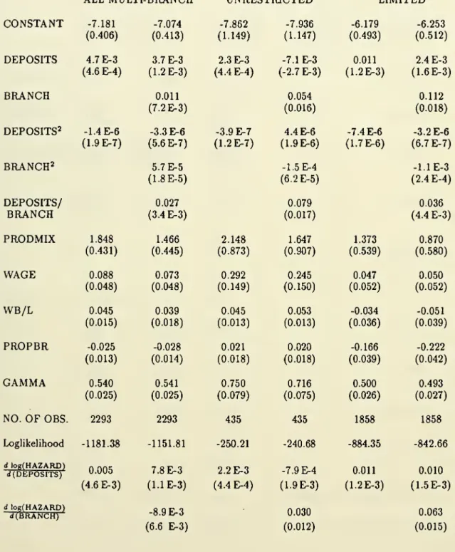
order statistic effect is addressed.

Weibull

estimates of the relationship

between

adoption

and

number

of

depos-itors are reported in

Table

2.

Pooled

estimates for

banks

in all states permitting multiple

branches

and

separate estimatesfor

banks

inlimited

and

unrestricted states

are reported.

The

results are consistent

with

the findings of

Hannan

and

McDowell:

the coefficients

imply

that the log of the

hazard

rate is

an

increasing,

concave

func-tion of

DEPOSITS.

The

estimates are precise,

and

the pattern is consistent across

regulatory regimes.

As

reported at the

bottom

of the table, these estimates

imply

that increasing

DEPOSITS

by

$1 million

above

the

sample

mean

leads to

about

an

0.5 percent increase in the

hazard

rate in the pooled regression.

The

increase is

more

marked

in limited

than

unrestricted states,

perhaps because

banks

in limited

states

have

much

smaller

DEPOSITS

on

average

and

the log of the

hazard

rate is

concave

in

DEPOSITS.

23

When

BRANCH

is included in the regressions it is entered as a quadratic

to allow it to

have

a curvature

independent

of

DEPOSITS.

As

suggested

by

the

model

in Section 2,

we

also include

DEPOSITS/BRANCH

to account for

location-specific costs of installing

ATMs.

The

sign

on

DEPOSITS/BRANCH

should

be

positive,

and

if location-specific costs are high relative to the

system

fixed costs, this coefficient

might

capture a large share of the effect of

DEPOSITS.

For

the

pooled

regression, the coefficients

on

the

BRANCH

terms

imply

that

adding a

branch

has - at best -

no

effect

on

the adoption rate.

The

derivative ofthe

log ofthe

hazard

rate

with

respect to

branch

is negative

with

a large

standard

error.

The

estimates for

banks

in unrestricted states, however, tell a very different story.

The

branch

derivative is positive in this regime. But, including the

BRANCH

variables

changes

the sign of the

DEPOSITS

derivative: the

apparent

effect of

an

increase in

DEPOSITS

holding

number

of branches constant is to

reduce

the

adoption

rate.

This

counterintuitive result

and

the

poor showing

of

BRANCH

in

the

pooled

regression

appear

to

be

the results ofnear colinearityof

DEPOSITS

and

BRANCH

in the unrestricted states.

The

correlation coefficient

between

BRANCH

and

DEPOSITS

for

banks

in

unrestricted states is .98. Apparently,

when

branching

is unrestricted,

banks

add

depositors

by adding

branches.

The

effect ofnear colinearity is reflectedin thelarge

increase in the

standard

errors

on

the

DEPOSITS

coefficients

when

BRANCH

is

added. In (unreported) regressions includingonly linear

DEPOSITS

and

BRANCH

23

All reported derivatives areevaluated at the

sample

means

for the observations included in the associated regression.