A new leading indicator of UK quarterly GDP growth

HAL Id: hal-00972860

https://hal-sciencespo.archives-ouvertes.fr/hal-00972860

Preprint submitted on 22 May 2014

HAL is a multi-disciplinary open access archive for the deposit and dissemination of sci-entific research documents, whether they are pub-lished or not. The documents may come from teaching and research institutions in France or

L’archive ouverte pluridisciplinaire HAL, est destinée au dépôt et à la diffusion de documents scientifiques de niveau recherche, publiés ou non, émanant des établissements d’enseignement et de recherche français ou étrangers, des laboratoires

Catherine Mathieu, Françoise Charpin

To cite this version:

Catherine Mathieu, Françoise Charpin. A new leading indicator of UK quarterly GDP growth. 2004. �hal-00972860�

A

N

L

I

UK

Q

GDP

G

N° 2004-10

Septembre 2004

Françoise C

Catherine

M

A

N

L

I

UK

Q

GDP

G

*

N° 2004-10

Septembre 2004

Françoise

C

**

Catherine

M

***

* This paper was prepared for the 27th CIRET Conference, Warsaw, September 2004.

** OFCE, Analysis and Forecasting Department and University of Paris II; E-mail: charpin@ofce.sciences-po.fr

*** OFCE, Analysis and Forecasting Department – 69, quai d’Orsay – 75340 Paris Cedex 07 – France; E-mail:catherine.mathieu@ofce.sciences-po.fr.

Abstract

This paper presents a new leading indicator of UK output growth. The aim of the indicator is to

forecast quarterly real GDP growth over a two-quarter horizon, using latest available information, mainly on a monthly basis, such as survey data, or on a daily basis, such as financial data (interest rates and exchange rates) and raw materials prices. We adopt a model where GDP

growth relies on the Index of Production,the Retail Sales Index, survey data in the manufacturing

sector, retail and wholesale trade, financial services and short-term interest rates. The indicator is built on a two-step regression-based approach. First, we estimate an equation for the quarterly GDP growth rate based on coincident and leading series. Second, we estimate monthly and/or quarterly equations which will be used to forecast the coincident and leading series showing a lead of less than six months. This enables us to forecast GDP growth for the current and coming quarters. We check that the indicator would have produced a satisfactory outcome over the last four years.

Keywords: Leading indicator, GDP, short-term forecasting JEL classification: E37

Résumé

Cet article présente un indicateur de croissance à court terme de l’économie britannique. Celui-ci permet de prévoir le taux de croissance trimestriel du PIB en utilisant des informations conjoncturelles : indices de production industrielle et des ventes de détail, enquêtes dans l’industrie, le commerce et les services financiers, taux d’intérêt. La démarche consiste dans un premier temps à estimer une équation économétrique donnant le taux de croissance du PIB en fonction de séries conjoncturelles coïncidentes ou avancées. On estime ensuite les équations permettant de prévoir les séries coïncidentes et celles dont l’avance est inférieure à six mois. On peut alors en déduire le taux de croissance du PIB à l’horizon de deux trimestres. Nous concluons la présentation de l’indicateur en vérifiant que son fonctionnement aurait été satisfaisant au cours des quatre dernières années.

1. Introduction

The objective of the paper is to build a leading indicator of UK output growth. The indicator will forecast quarterly real GDP growth over a two-quarter horizon, using the latest available information, mainly on a monthly basis such as survey data, or on a daily basis such as financial data (interest rates and exchange rates) and raw materials prices. These types of leading indicators provide an alternative method of forecasting short-term movements in activity, complementing structural macro-econometric models and cyclical analysis derived from the NBER approach focusing on turning point detection.

In the UK, the Office for National Statistics (ONS) releases three quarterly GDP estimates in a quarter: a preliminary estimate of quarter Q is available at the end of the first month of quarter (Q+1); a second estimate at the end of the second month of quarter (Q+1); a third estimate at the end of the third month of the quarter (Q+1). These release dates are very close to the US ones.1 These are short delays in international standards, for instance as compared with euro area countries, even though delays have been shortened recently in the area. A first estimate for euro area GDP in quarter Q is now available 45 days after the end of the quarter.2

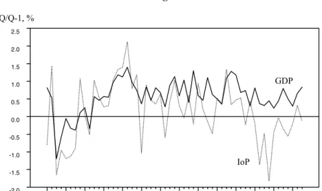
We implement a two-step regression-based approach, following work done at OFCE by Charpin (2001) for the US, Charpin (2002) for the euro area and Heyer and Péléraux (2004) for France. First, we estimate an equation linking the quarterly GDP growth rate to rapidly available information. Hence monthly series will be preferred, but quarterly series may be also included if they are leading. The introduction of coincident series will be avoided, except when absolutely needed, as will be the case for the index of the output of the production industries and the Retail Sales Index. It may be noted that the ONS uses these two indexes plus limited information on the output of the rest of the economy to produce the first quarterly GDP estimate.3 We adopt a similar approach. Figure 1 illustrates how GDP and the Index of Production moved in line until 1997. Since then, the link has become less obvious. In particular, the industrial recession initiated at the beginning of 2001 is very partially reflected on GDP growth which is unusual as compared with the last 25 years. The robustness of activity in services, among them financial services and

1 Although in the UK the first – so called preliminary - estimate of GDP applies to aggregate GDP only, whereas in the US the advance estimate of GDP is released together with a large set of national accounts data.

2 Two years ago the first estimate for quarter Q was released in the first fortnight of the last month of quarter (Q+1). 3 The preliminary estimate is based on information covering 45% of value added (Reed, 2002).

retail trade, and, more recently, in the construction sector have helped compensate for the negative impact of the fall in industrial activity on GDP. Besides, figure 2 shows a sharp acceleration in retail sales growth in 2000 whereas GDP growth was decelerating. The disconnection between GDP, IoP and retail sales growth rates has strengthened since the autumn 2003 revision of national accounts and retail sales (see box). Second, we estimate monthly and/or quarterly equations which will be used to forecast the coincident and leading series showing a lead of less than six months. This will enable us to predict GDP growth for the current and following quarters.

We adopt a model where output growth is related to the index for the output of the production industries (IoP), capacity utilisation, the Retail Sales Index (RSI), a wholesale trade survey factor, a financial survey factor and short-term interest rates. The IoP, capacity utilisation and the RSI are coincident and therefore need to be forecast. These three variables will be linked to survey data, the IoP and capacity utilisation being also related to interest rates and, for the latter, to real oil prices.

There is to our knowledge no similar quarterly GDP leading indicator for the UK. However the NIESR produces a monthly GDP indicator for GDP growth of the last three months and hence provides a rolling forecast of last 3 months growth (Mitchell et al., 2004). At the beginning of quarter (Q+1), following the IoP’s release for the second month of quarter Q, the indicator produces a first estimate of GDP for quarter Q, two weeks before the official preliminary estimate of GDP. One month later, the indicator will provide the average GDP growth for months (M-3) to (M-1) as compared to three months earlier. It is therefore a very short-term forecast. The method consists in estimating monthly equations for the main output components.

Section 2 presents the forecasting equation for the GDP growth rate. The forecasting equations for the coincident and leading variables are shown in section 3. Section 4 analyses the out-of-sample forecasting errors for the last four years. Section 5 concludes.

Figure 1 GDP and Index of Production growth rates Q/Q-1, %

Source: ONS.

Figure 2 GDP and Retail Sales Index growth rates Q/Q-1, % Source: ONS. 1990 1991 1992 1993 1994 1995 1996 1997 1998 1999 2000 2001 2002 2003 -2.0 -1.5 -1.0 -0.5 0.0 0.5 1.0 1.5 2.0 2.5 IoP GDP 1990 1991 1992 1993 1994 1995 1996 1997 1998 1999 2000 2001 2002 2003 -2.0 -1.5 -1.0 -0.5 0.0 0.5 1.0 1.5 2.0 2.5 Retail sales GDP

Box: An illustration of data revisions on GDP and Retail Sales Index

The ONS introduced chained volumes in quarterly national accounts in September 2003. The effect of annual chain-linking on annual real GDP growth rates is estimated to be small: Tuke and Beadle (2003) estimate the impact to be +0.2 percentage point in 1995, 0.0 from 1996 to 1998 and -0.1 in 1999 and 2000. But national accounts also include revisions due to the adoption of a new base year (2000 instead of 1995) and these revisions are estimated to have raised annual real GDP growth by 0.3 percentage point on average over the last five years. The revisions in quarterly growth rates are significant (see figure 1).

Figure 1 Quarterly GDP growth rates before and after September 2003 revision

Q/Q-1, %

Source: ONS.

In October 2003 the Retail Sales Index was also significantly revised starting from January 2000 (Cope and Davies, 2003). Figure 2 shows that sales now appear to have risen more rapidly and with increased volatility in the early 2000’s than previously thought.

Figure 2 Quarterly RSI growth rates before and after October 2003 revision

Q/Q-1, % Source: ONS. 1986 1988 1990 1992 1994 1996 1998 2000 2002 -1.5 -1.0 -0.5 0.0 0.5 1.0 1.5 2.0 2.5 Retail sales

Retail sales (old) (dotted line) 1986 1988 1990 1992 1994 1996 1998 2000 2002 -1.5 -1.0 -0.5 0.0 0.5 1.0 1.5 2.0 2.5 GDP GDP (old) (dotted line)

2. The quarterly GDP growth rate equation

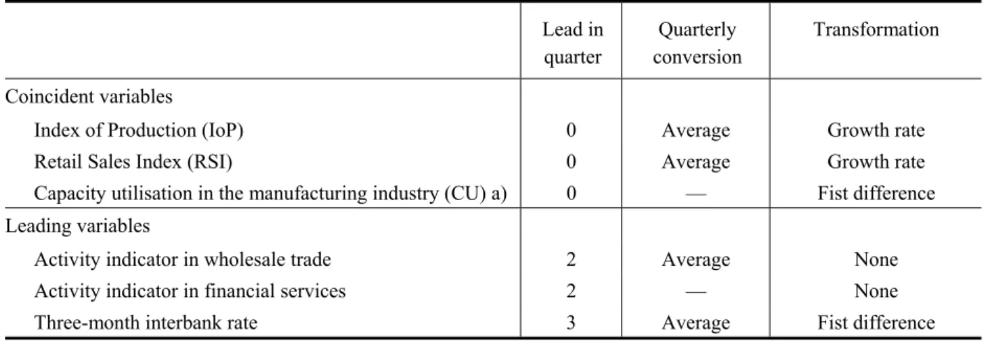
The list of the right hand side (RHS) variables of the equation is shown in table 1. The conversion to quarterly data (quarterly average or end of quarter) and the transformation operated on the variable (first difference, growth rate or none) are also given. After transformation, the series will be assumed to be stationary. Three main types of variables 4 can be found in the equation:

- Activity indexes: monthly index for the output of the production industries, monthly Retail Sales Index

- Survey data: quarterly survey on capacity utilisation in the manufacturing sector, monthly wholesale trade survey, financial services quarterly survey

- Financial data: the three-month interbank rate.

Table 1. Coincident and Leading Variables in the GDP growth rate equation Lead in quarter Quarterly conversion Transformation Coincident variables

Index of Production (IoP) 0 Average Growth rate

Retail Sales Index (RSI) 0 Average Growth rate

Capacity utilisation in the manufacturing industry (CU) a) 0 — Fist difference

Leading variables

Activity indicator in wholesale trade 2 Average None

Activity indicator in financial services 2 — None

Three-month interbank rate 3 Average Fist difference

Note: a) % of firms working at full capacity.

Sources: Bank of England, CBI, ONS, authors’ calculations.

The indicator is linked to variables illustrative of activity in the industry5 (23% of total value added in 2000), retail and wholesale trade (12%, including motor trade) and financial services (5.4%), i.e. about one third of GDP. Although one may have expected construction

4 Data sources are detailed in Appendix 1.

5 The index of Production covers manufacturing output (79% of total index in 2001), mining and quarrying (12%), electricity gas and water (9%).

sector’s variables to play a role (housing starts, orders received….) this did not turn out to be the case.

It would have been preferable to use an activity indicator based on the monthly industrial survey rather than the Index of Production (IoP) itself and an activity indicator based on the monthly retail trades survey rather than the Retail Sales Index (RSI), because survey data for a given month are released one month earlier than the IoP and the RSI of the same month and are not revised. But the activity indicator built as the first factor of a principal component analysis (PCA) carried out on the monthly industrial survey did not turn out to be as econometrically significant as IoP in the GDP growth equation. 6 This was also true for the activity indicator in retail trade as compared with the RSI. They will nevertheless prove useful for the monthly forecasts of the coincident variables. The absence of industrial survey data in the GDP growth rate equation is a British specificity as compared with the indicators built at OFCE for the US, the euro area and France.

Capacity utilisation in the manufacturing sector is derived from the quarterly series giving the percentage of firms working below capacity, according to the CBI industrial trends survey. In the equation, we consider the percentage of firms working at full capacity, which will be denoted as CU in the rest of the paper. Table 1 says this variable is coincident. However, when the GDP figure for quarter Q is released, CU is available for quarter (Q+1).7 Hence it will need to be forecast one-quarter ahead only to compute GDP forecast for quarter (Q+2).

The activity indicator in wholesale trade is the first factor of a PCA carried out on the four series of the monthly CBI survey relating to expected volume of sales for the month to come, orders placed, stocks, sales for the time of the year. As some of these series might be trended, they are all detrended before carrying out the PCA over the 1985-2003 period.

The activity indicator in the financial services is built in a similar way. We consider the first factor of a PCA carried out on the eight series of the quarterly CBI/PWC Pricewaterhouse

Coopers financial services survey. This survey was launched in the 4th quarter of 1989 only and

this will shorten our sample period. The growth rate of a UK equity price index could have been

6 The UK purchasing managers’ index (PMI) was also tested, although the series starts in 1991. Its coefficient was not significantly different from 0.

7 The survey is conducted at the beginning of the quarter and published at the end of the first month of the same quarter.

introduced in the equation instead, but the activity indicator of financial services was more significant econometrically.

Interest rates spreads are generally considered as GDP growth predictors in the literature. But in the UK the spread reflects at the beginning of our sample the episode of the EMS membership. From October 1990 to September 1992 the short-term rate was maintained at unusually high levels before falling abruptly once the British Pound left the exchange rate mechanism. Monetary policy plays a role in the equation through the change in nominal short-term interest rates.

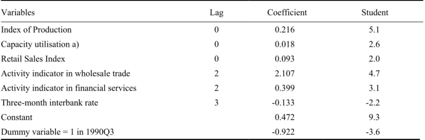
The equation is shown in table 2. All variables have coefficients significantly different from 0 with the expected sign. The introduction of a dummy variable in 1990Q3 was necessary because the sharp fall in GDP at the trough of the 1990’s recession could not be satisfactorily explained. The 1990q3 ‘extreme’ value could have possibly affected the selection of RHS variables and the value of their estimated coefficients if a dummy variable had not been introduced.

The IoP plays a major role in the equation. Conversely, the RSI has seen its impact on GDP decline in recent years and is not as strongly correlated with GDP growth as in the past. It remains to be seen whether the recent disconnection between GDP and RSI fluctuations will persist in the future (see figure 2). The increased volatility of the RSI since the 2003 revision also raises questions. Before this revision the index was clearly econometrically significant in the equation. But the ONS says it still uses the RSI to construct the preliminary GDP estimate…

The activity indicator in wholesale trade plays a significant role. Retail trade is present in the equation via the RSI. But the latter have seen their impact reduced and, anyway, are coincident whereas wholesale trade activity has a lead of 2 quarters.

The quarterly activity indicator in financial services also plays a significant role in the equation and has a 2 quarter lead. This role may be due to the size of financial services in the British economy.

Last, a 1 percentage point rise in the three-month interbank interest rate will lower quarterly GDP growth by 0.13% after 3 quarters.

Table 2 . Equation for the quarterly GDP growth rate

Variables Lag Coefficient Student

Index of Production 0 0.216 5.1

Capacity utilisation a) 0 0.018 2.6

Retail Sales Index 0 0.093 2.0

Activity indicator in wholesale trade 2 2.107 4.7

Activity indicator in financial services 2 0.399 3.1

Three-month interbank rate 3 -0.133 -2.2

Constant 0.472 9.3

Dummy variable = 1 in 1990Q3 -0.922 -3.6

Note: a) % of firms working at full capacity in the manufacturing sector. Sample period: 1990Q2-2003Q3; R2 = 0.82 DW = 2.3 SEE = 0.23%. Source: Authors’ estimates.

Figure 3 shows actual and fitted GDP growth rates. The estimate plotted for 1990Q3 does not account for the dummy variable. The figure shows that GDP growth fluctuations are not perfectly estimated. For instance, growth is underestimated in the first half of 1994, and slowdowns earlier than actual growth at the turn of 1999/2000. GDP growth is also underestimated in the first half of 2002. The estimate frequently minors actual fluctuations, leading residuals to switch alternatively from negative to positive signs. That is why there is a certain negative residual autocorrelation.

Figure 3 Actual and fitted GDP growth rates (equation 2) Q/Q-1, %

Sources: ONS, authors’ estimates.

1990 1991 1992 1993 1994 1995 1996 1997 1998 1999 2000 2001 2002 2003 -1.5 -1.0 -0.5 0.0 0.5 1.0 1.5 Actual

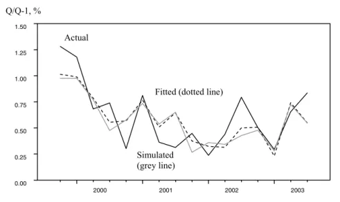
It is important to check, here with an informal method, the stability of the equation. Therefore, we have estimated the equation on a sample ending in 1999Q3. We have then simulated GDP growth from 1999Q4 to 2003Q3. Figure 4 shows these simulated GDP growth rates together with the fitted values of the equation run over the whole sample period. It can be seen that the two series are very close, which allows us to think that the equation is stable.

Figure 4 Actual, fitted and simulated GDP growth rates Q/Q-1, %

Sources: ONS, authors’ estimates.

3. Forecasts of the coincident variables

Let Q stand for the last quarter known. The indicator will forecast (Q+1) and (Q+2) GDP growth rates. The first GDP estimate for quarter Q is released by the ONS at the end of the first month (M1) of quarter (Q+1). Two weeks later, i.e. in the second week of the second month (M2) of (Q+1) the Index of Production for the third month (M3) of quarter Q is released. Just after the IoP’s release, we will run the first forecast for (Q+1) and (Q+2) GDP growth rates. At that moment the last known RSI value is for the third month of quarter Q. Hence, neither the IoP nor the RSI, the two coincident variables of the equation, provide information on (Q+1). However, this first forecast of GDP growth will be revised at the beginning of the two following months8 to embed latest available information, which will then bear on the first and second months of quarter (Q+1). Under this time schedule, the GDP forecasts for (Q+1) (respectively (Q+2)) will

2000 2001 2002 2003 0.00 0.25 0.50 0.75 1.00 1.25 1.50 Simulated (grey line)

Fitted (dotted line) Actual

require to forecast the Index of Production and the Retail Sales Index at a 3, 2, 1 month horizon (respectively at a 6, 5, 4 month horizon) depending on the forecasting date.

Capacity utilisation is known for (Q+1) when GDP for Q is released. Hence it does not need to be forecast when forecasting (Q+1) GDP, but it needs to be forecast one-quarter ahead for the (Q+2) GDP forecast.

3.1 Forecasting equations for the monthly IoP growth rate

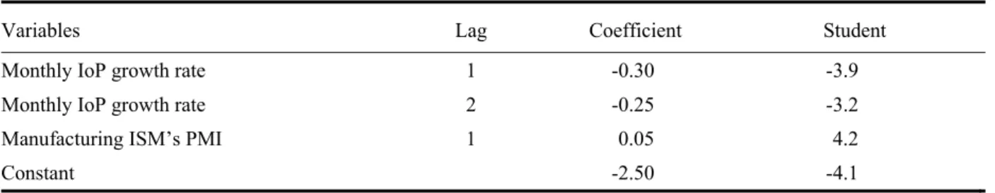
The IoP and and the RSI will be modelled in growth rates as the two series are I(1) with a drift. The forecasting equation for the monthly IoP growth rate is shown in table 3. IoP will be linked to past IoP growth, with two lags, and to activity in the US manufacturing sector, measured as the manufacturing ISM’s Purchasing managers’ index (PMI), with one lag. We use the fact that US industrial activity has some lead on UK industrial activity. The equation explains only 15% of the monthly IoP growth rate, which is a very volatile series (see figure A2.1 in Appendix 2). The equation represents the trend in industrial activity only.

Table 3 . Forecasting equation for the monthly IoP growth rate

Variables Lag Coefficient Student

Monthly IoP growth rate 1 -0.30 -3.9

Monthly IoP growth rate 2 -0.25 -3.2

Manufacturing ISM’s PMI 1 0.05 4.2

Constant -2.50 -4.1

Sample period: January 1990-November 2003; R2 = 0.15 DW = 2.0. Source: Authors’ estimates.

The US ISM’s PMI is known for month (M+1) when M is the latest month available for UK IoP. Hence, forecasting IoP for the (M+h) month requires to forecast the US PMI for (M+h-2). This forecast will be run using the equation shown in table 4. The level of the US PMI is modelled as the series is stationary. The equation is autoregressive of order 4 and includes the US interest rates spread as economic activity predictor. The equation can be rewritten with the following regressors: the first lag of the ISM’s PMI in level and the first three lags of its first difference. These new variables have positive coefficients. Owing to the strong autoregressivity

8 Respectively at the beginning of the third month of quarter (Q+1) and at the beginning of the first month of quarter (Q+2), just after the IoP’s release.

of the PMI and to its low volatility, forecasts will be satisfactory, except possibly at cyclical turning points.

Table 4 . Forecasting equation for monthly US manufacturing activity (ISM’s PMI)

Variables Lag Coefficient Student

ISM’s PMI 1 0.95 13.6

ISM’s PMI 2 -0.01 -0.1

ISM’s PMI 3 0.06 0.7

ISM’s PMI 4 -0.18 -2.5

US interest rates spread (ten-year – three-month) 4 0.37 2.6

Constant 8.5 4.9

Dummy variable = 1 in October 2001 -8.1 -4.2

Dummy variable = 1 in March 2003 -5.2 -2.7

Sample period: January 1988-December 2003; R2 = 0.85 DW = 1.9. Source: Authors’ estimates.

3.2 Forecasting equations for the monthly RSI growth rate

The forecasting equation for the monthly RSI growth rate is shown in table 5. The right-hand-side variables are past RSI growth rates, with two lags, the change in the UK industrial activity indicator with one lag, and the indicator of retail trade activity with a four month lag. The industrial activity indicator is the first factor of a PCA carried out on the CBI survey after treatment of the European Commission,9 based on five questions: production expectations, order books, stocks of finished products, production trend observed in recent months and export order books. Only 27% of the RSI is explained by the equation. The RSI is a very volatile series as can be seen from figure A2.2 in Appendix 2, where observed and fitted RSI values are shown. As said above for the IoP, the model captures only the trend growth of the dependent variable.

9 We have chosen the series published by the European Commission rather than by the CBI, because the former include one question which is not released on a monthly basis by the CBI: recent trends in production.

Table 5. Forecasting equation for the monthly RSI growth rate

Variables Lag Coefficient Student

Monthly RSI growth rate 1 -0.53 -7.0

Monthly RSI growth rate 2 -0.16 -2.1

Change in industrial activity indicator (first difference) 1 4.54 3.2

Activity indicator in retail trade 4 1.62 3.1

Constant 0.49 7.3

Sample period: January 1990-November 2003; R2 = 0.27 DW = 2.0. Source: Authors’ estimates.

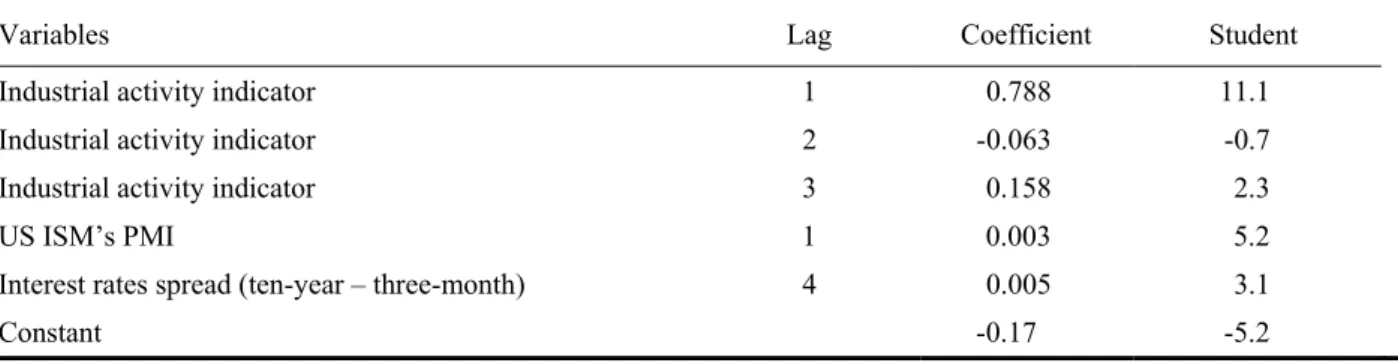
When the RSI of month M is released, the industrial activity indicator is available for month (M+1). Hence, we need to forecast the industrial activity up to (M+h-2) to be able to forecast the RSI for (M+h). This forecast is run with the equation shown in table 6, where the industrial activity indicator is modelled in level, as the variable is stationary.

Table 6 . Forecasting equation for monthly UK industrial activity indicator

Variables Lag Coefficient Student

Industrial activity indicator 1 0.788 11.1

Industrial activity indicator 2 -0.063 -0.7

Industrial activity indicator 3 0.158 2.3

US ISM’s PMI 1 0.003 5.2

Interest rates spread (ten-year – three-month) 4 0.005 3.1

Constant -0.17 -5.2

Sample period: January 1988-December 2003; R2 = 0.94 DW = 2.0. Source: Authors’ estimates.

The equation is autoregressive of order 3 and can be rewritten using as regressors: the first lag of the dependent variable and the first and second lags of its first difference, in order to have positive and statistically significant coefficients. Unsurprisingly, the UK industrial activity indicator has a one month lag with the US indicator. Last, the interest rates spread plays a role as a growth predictor. Owing to the strong autoregressivity of the industrial activity indicator, forecasts will give a satisfactory outcome, except possibly at turning points. The presence of the US PMI with a one-month lead should facilitate the prediction of turning points. To forecast UK

industrial activity growth at a four-month horizon – which is the maximum needed – it is necessary to forecast the US PMI for 3 months. The forecasting equation is given in table 4.

3.3 Forecasting equation for the quarterly change in capacity utilisation

The change in capacity utilisation needs to be forecast one-quarter ahead only and will be used when forecasting (Q+2) GDP growth. The equation giving the change in capacity utilisation is shown in table 7. The equation is autoregressive. The change in CU is forecast using the one-quarter lag of the change in the industrial activity indicator, interest rates spreads with a three-quarter lag and three-quarterly real oil prices growth rates, with a three-three-quarter lag. A rise in real oil prices will have a negative impact on the capacity utilisation indicator. Only 37% of the observed change in CU is explained by the equation, quarterly changes in CU being rather volatile. Actual and fitted changes in CU can be seen on figure A2.3, Appendix 2.

Table 7. Forecasting equation for change in capacity utilisation

Variables Lag Coefficient Student

Change in CU (first difference) 1 -0.30 -2.6

Change in industrial activity indicator (first difference) 1 39.8 4.5

Interest rates spread (ten-year – three-month) 3 0.69 2.4

Real oil prices, quarterly growth rate 3 -0.07 -2.1

Constant -0.17 -0.4

Sample period: 1988Q1-2003Q4; R2 = 0.37 DW = 2.2. Source: Authors’ estimates.

In conclusion of this section, it may be noted that there is a substantial forecasting exercise to be done on coincident variables in comparison with the indicators built at OFCE (USA, euro area, France). It may also be wondered if these forecasts will not deteriorate the GDP growth rate forecasts. We will see in the following section that forecasting errors on GDP growth remain close to the errors of the GDP growth rate equation.

4. Out-of-sample forecasting errors for the last four years

This section analyses the out-of-sample forecasting errors which would have resulted from running the set of equations presented above, from the end of 1999 to the end of 2003. The first forecast was run at the beginning of November 1999, with the quarterly GDP growth rate equation estimated from 1990Q2 to 1999Q3. The forecasting equation for CU was estimated up

to 1999Q4 while forecasting equations for monthly IoP and RSI growth rates were estimated up to September 1999. The first forecasted quarters are 1999Q4 and 2000Q1. These two quarters will be forecast again in early December 1999 and early January 2000, with monthly equations being re-estimated so as to embed latest information. We will repeat the exercise to forecast GDP growth for the first two quarters of 2000, first in February 2000, then in March and in April. This will be done again until August, September and October 2003 when the three forecasts for 2000Q3 and 2000Q4 are run. We will then have 48 forecasting errors available for the one-quarter ahead forecast (16 for each month) and, similarly, 48 forecasting errors for the two-quarter ahead forecast. These calculations have been done using revised and not real-time data.

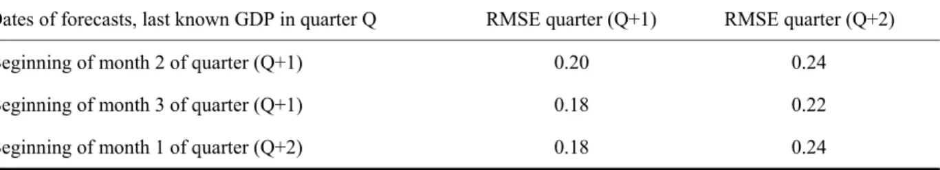
Table 8 shows the root mean squared errors according to the forecast quarter and the forecasting date of the month. These errors can be compared with the residuals of the regression

equation on the same period – equal to 0.19. It can be seen that for the two forecast quarters

forecasting errors are similar to the error of the regression equation, even though they are somewhat larger for the two-quarter ahead forecast. Figures 5 and 6 illustrate these elements.

Table 8. Root mean squared errors depending on forecasting horizons Percentage point

Dates of forecasts, last known GDP in quarter Q RMSE quarter (Q+1) RMSE quarter (Q+2)

Beginning of month 2 of quarter (Q+1) 0.20 0.24

Beginning of month 3 of quarter (Q+1) 0.18 0.22

Beginning of month 1 of quarter (Q+2) 0.18 0.24

Source: Authors’ estimates.

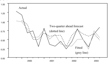
Figure 5 shows GDP growth forecasts for quarter (Q+1) run at the beginning of the third month of quarter (Q+1) – middle date – and fitted GDP growth. The two plots are very close at the exception of 2 quarters (2001Q3 and 2002Q2) where the forecast performs better than fitted values. Figure 6 shows the same comparison for the two-quarter ahead forecast run at the beginning of the third month of quarter (Q+1) – middle date – and fitted GDP growth. Four major between the plots may be noted. The forecast for 2001Q4 is significantly higher than fitted GDP growth, which can be explained by the fact that the forecast was run early in September 2001, before the 11 September 2001 attacks. The forecast is also higher than fitted GDP growth for 2003Q1, which can be explained by the fact that the forecast was run in early December, before

the start of the war in Irak. In the end, 2 differences between the forecasted and fitted values remain ‘unexplained’: 2002Q2 and 2002Q3, but then the forecasting errors compensate for the weakness of the equation.

Figure 5 Actual, fitted and one-quarter-ahead forecast GDP growth rates over the last four years (middle date)

Q/Q-1, %

Sources: ONS, authors’ estimates.

Figure 6 Actual, fitted and two-quarter-ahead forecast GDP growth rates over the last four years (middle date)

Q/Q-1, %

Sources: ONS, authors’ estimates.

2000 2001 2002 2003 0.00 0.25 0.50 0.75 1.00 1.25 1.50

Two-quarter ahead forecast (dotted line) Fitted (grey line) Actual 2000 2001 2002 2003 0.00 0.25 0.50 0.75 1.00 1.25 1.50 Actual

One quarter-ahead forecast (dotted line)

Fitted (grey line)

Figure 7 shows the three forecasts run for one-quarter ahead GDP growth. The first forecast, run at the beginning of the second month of quarter (Q+1) is less reliable than the two others, especially in 2003Q1. This forecast is supposed to be run at the beginning of February 2003 and relies on information available up to December 2002, which did not include the effects of the war in Iraq. Figure 8 shows that the three forecasts run at the two-quarter ahead horizon are very similar. These figures suggest that forecasting errors occur either in exceptional circumstances (11 September 2001, war in Irak) or result from the regression equation. Forecasting the coincident variables does not substantially deteriorate the forecasting performance of the GDP growth rate equation.

Figure 7 Actual and one-quarter-ahead forecast GDP growth rates over the last four years

Q/Q-1, %

Sources: ONS, authors’ estimates.

2000 2001 2002 2003 0.00 0.25 0.50 0.75 1.00 1.25 1.50 Actual Month 3, quarter Q+1 (dotted line) Month 1, quarter Q+2 (grey line) Month 2, quarter Q+1 (thin dotted line)

Figure 8 Actual and two-quarter-ahead forecasts GDP growth rates over the last four years

Q/Q-1, %

Sources: ONS, authors’ estimates.

5. Conclusion

The main weakness of this indicator is that it does not provide fully satisfactory estimates of quarterly GDP fluctuations. The strength of the indicator is the stability of the equation, ensured by the introduction of two coincident variables – the Index of Production and the Retail Sales Index – which are part of the GDP. The counterpart is that the two variables need to be forecast. However, we have shown that forecasting errors on these two variables have had a limited impact on GDP forecast over the last four years.

The main advantage of this type of leading indicator is to provide quantified quarterly GDP growth, available on a monthly basis: three monthly estimates may be produced for a given quarter, embedding the most recent information available. Besides, contributions of the RHS variables will provide an indication on how different sectors of the economy respectively affect quarterly output growth.

UK output growth is a priori a good candidate for implementing leading indicators because of the large pool of variables, especially in terms of surveys. But the methodology may easily be implemented to other economies. In particular, it may prove most useful for short-term analysis in countries where GDP is released with delay. Another advantage of the method is that equations do not need to be estimated over a long time period. Starting the estimation in the late 1980’s

2000 2001 2002 2003 0.00 0.25 0.50 0.75 1.00 1.25 1.50 Actual Month 3, quarter Q+1 (dotted line) Month 2, quarter Q+1 (thin dotted line) Month 1, quarter Q+2

seems reasonable for UK GDP. This type of tool may therefore prove useful for short-term analysis in Central and Eastern European economies.

References

Charpin, F. (2002), ‘Un indicateur de croissance à court terme de la zone euro’, Revue de

l’OFCE, No. 83, October, pp. 229-242.

Charpin, F. (2001), ‘Un indicateur de croissance à court terme aux Etats-Unis’, Revue de

l’OFCE, No. 79, October, pp. 171-189.

Cope, I. and Davies, P. (2003), ‘Retail Sales Index development’, Economic Trends, No. 601, December, pp. 31-35.

Heyer, E. and Péléraux, H. (2004), ‘Un indicateur de croissance infra-annuelle pour l’économie française’, Revue de l’OFCE, No. 88, January, pp. 203-218.

Mitchell, J., Smith, R. J., Weale, M. R., Wright, S. and Salazar, E. L. (2004), ‘An indicator of monthly GDP and an early estimate of quarterly GDP growth,’ NIESR Discussion Paper 127 (revised).

Reed, G.(2002), ‘How much information is in the UK preliminary estimate of GDP?’,Economic

Trends, No. 585, August, pp. 57-64.

Tuke, A. and Beadle, J. (2003), ‘The effect of annual chain-linking on Blue Book 2002 annual growth estimates’, Economic Trends, No. 593, April, pp. 29-40.

Appendix 1 - Data sources

Most of the data used in this article are produced by the ONS and the CBI. All data have been taken from Datastream and their mnemonics are given in the table below.

Source ONS Code Datastream Code

GDP, chained volume, SA ONS ABMI UKABMI..

Index of Production, chained volume, SA ONS CKYW UKCKYW..

Retail Sales Index, volume, SA ONS EAPS UKEAPS..

% of firms working below capacity, manufacturing sector

CBI — UKCBICAB

Activity indicator in financial services CBI/PWC a) — UKCBIFXX

where XX = LB, DO, DM, LO, OP, ST, VF, VB

Activity indicator in wholesale trade CBI — UKCBWXXB

where XX = SE, DE, TE, KE

Activity indicator in retail trade CBI — UKCBRXXB

where XX = SE, DE, TE, KE

Industrial activity indicator European

Commission

— UKEUSIXXQ

where XX = PR, OB, EB, FP, PA

Three-month interbank rate BoE/ONS AMIJ UKAMIJ..

Gross redemption yield on ten-year gilt edged stocks

Datastream — UKMEDYLD

Oil prices IMF — WDI76AAZA

Producer price index (manufactured products)

ONS PLLU UKPLLU..

Manufacturing purchasing managers’ index (PMI-ISM), US

Institute for supply management

— USCNFBUSQ

Three-month US Treasury bill Federal reserve — USTRB3AV

Ten-year US Treasury bill Federal reserve — USTRCN10

Appendix 2

Figure A2.1 Index of Production: actual and fitted growth rates M/M-1, %

Sources: ONS, authors’ estimates.

Figure A2.2 Retail Sales Index: actual and fitted growth rates M/M-1, %

Sources: ONS, authors’ estimates.

1990 1991 1992 1993 1994 1995 1996 1997 1998 1999 2000 2001 2002 2003 -2.4 -1.6 -0.8 -0.0 0.8 1.6 2.4 Actual Fitted (in bold) 1990 1991 1992 1993 1994 1995 1996 1997 1998 1999 2000 2001 2002 2003 -2.5 -2.0 -1.5 -1.0 -0.5 0.0 0.5 1.0 1.5 2.0 Actual Fitted (in bold)

Figure A2.3 Capacity utilisation: actual and fitted Q/Q-1, First difference, Percentage points

Sources: CBI, authors’ estimates.

1990 1991 1992 1993 1994 1995 1996 1997 1998 1999 2000 2001 2002 2003 -12.5 -10.0 -7.5 -5.0 -2.5 0.0 2.5 5.0 7.5 10.0 Actual Fitted (dotted line)

Appendix 3 - Equation for the quarterly GDP growth rate: An update

Table A3.1 shows the latest results available for the GDP growth rate, i.e. for the equation run on 7 September 2004, following the release of IoP’s data for July. The two-quarter-ahead forecast is shown in figure A3.1.

Table A3.1 Equation for the quarterly GDP growth rate

Variables Lag Coefficient Student

Index of Production 0 0.222 5.4

Capacity utilisation a) 0 0.015 2.0

Retail Sales Index 0 0.123 2.9

Activity indicator in wholesale trade 2 2.245 5.0

Activity indicator in financial services 2 0.371 2.8

Three-month interbank rate 3 -0.134 -2.2

Constant 0.476 9.3

Dummy variable = 1 in 1990Q3 -0.897 -3.4

Note: a) % of firms working at full capacity in the manufacturing sector. Sample period: 1990Q2-2004Q2; R2 = 0.81 DW = 2.3 SEE = 0.23%. Source: Authors’ estimates.

Figure A3.1 Actual and fitted GDP growth rates (equation A3.1) Q/Q-1, % -1,5 -1,0 -0,5 0,0 0,5 1,0 1,5 1990 1991 1992 1993 1994 1995 1996 1997 1998 1999 2000 2001 2002 2003 2004 GDP 04q2 (August 2004)

Fitted (dotted line)

Forecast