HAL Id: hal-02113864
https://hal.archives-ouvertes.fr/hal-02113864
Submitted on 29 Apr 2019
HAL is a multi-disciplinary open access
archive for the deposit and dissemination of
sci-entific research documents, whether they are
pub-lished or not. The documents may come from
teaching and research institutions in France or
abroad, or from public or private research centers.
L’archive ouverte pluridisciplinaire HAL, est
destinée au dépôt et à la diffusion de documents
scientifiques de niveau recherche, publiés ou non,
émanant des établissements d’enseignement et de
recherche français ou étrangers, des laboratoires
publics ou privés.
Algorithms for the Sequential Reprogramming of
Boolean Networks
Hugues Mandon, Cui Su, Jun Pang, Soumya Paul, Stefan Haar, Loïc Paulevé
To cite this version:
Hugues Mandon, Cui Su, Jun Pang, Soumya Paul, Stefan Haar, et al.. Algorithms for the
Se-quential Reprogramming of Boolean Networks. IEEE/ACM Transactions on Computational
Biol-ogy and Bioinformatics, Institute of Electrical and Electronics Engineers, 2019, 16 (5), pp.1610-1619.
�10.1109/TCBB.2019.2914383�. �hal-02113864�
Algorithms for the Sequential Reprogramming of
Boolean Networks
Hugues Mandon
∗†, Cui Su
‡, Jun Pang
§‡, Soumya Paul
§, Stefan Haar
∗, Lo¨ıc Paulev ´e
†¶ ∗LSV, ENS Cachan, INRIA, CNRS, Universit ´e Paris-Saclay, France
†
LRI UMR 8623, Univ. Paris-Sud – CNRS, Universit ´e Paris-Saclay, France
‡SnT, University of Luxembourg
§
FSTC, University of Luxembourg
¶
Univ. Bordeaux, Bordeaux INP, CNRS, LaBRI, UMR5800, F-33400 Talence, France
Abstract—Cellular reprogramming, a technique that opens huge opportunities in modern and regenerative medicine, heavily relies on
identifying key genes to perturb. Most of the existing computational methods for controlling which attractor (steady state) the cell will reach focus on finding mutations to apply to the initial state. However, it has been shown, and is proved in this article, that waiting between perturbations so that the update dynamics of the system prepares the ground, allows for new reprogramming strategies. To identify such sequential perturbations, we consider a qualitative model of regulatory networks, and rely on Binary Decision Diagrams to model their dynamics and the putative perturbations.
Our method establishes a set identification of sequential perturbations, whether permanent (mutations) or only temporary, to achieve the existential or inevitable reachability of an arbitrary state of the system. We apply an implementation for temporary perturbations on models from the literature, illustrating that we are able to derive sequential perturbations to achieve trans-differentiation.
F
1
I
NTRODUCTIONR
EGENERATIVE medicine has gained traction with the discovery of cell reprogramming, a way to change a cell phenotype to another, allowing tissue or neuron regen-eration techniques. After proof that cell fate decisions could be reversed [21], scientists need efficient and trustworthy methods to achieve cell reprogramming. Instead of pro-ducing induced pluripotent stem cells and force the cell to follow a distinct differentiation path, new methods focus on trans-differentiating the cell, without necessarily going (back) through a multipotent state [7], [6].This paper addresses the formal prediction of perturba-tions for cell reprogramming from computational models of gene regulation. We consider qualitative models where the genes and/or the proteins, notably transcription factors, are variables with an assigned value giving the level of activity, e.g., 0 for inactive and 1 for active, in a Boolean abstraction. The value of each variable can then evolve in time, depending on the value of its regulators.
In qualitative models of gene regulation, attractors of the dynamics, which represent the long term dynamics, are typically associated with differentiated and/or stable states of the cell [14], [22]. In such a setting, cell reprogram-ming can be interpreted as triggering a change of attractor: starting within an initial attractor, perform perturbations which would de-stabilize the network and lead the cell to a different attractor.
Current experimental settings and computational mod-els mainly consider cell reprogramming by applying the set of perturbations simultaneously in the initial state. How-ever, as suggested in [18] and as we will demonstrate formally in this paper, one finds novel reprogramming strategies, potentially requiring fewer interventions and / or achieving more objectives, by using sequential
reprogram-ming, i.e., where perturbations are applied at particular points in time, and in a particular ordering.
Contribution: This paper establishes the formal char-acterization of all possible reprogramming paths leading from one state of an asynchronous Boolean network to an-other, by means of a bounded number of either permanent (mutations) or temporary perturbations. We will account for whether the target state may be reached, or will be reached inevitably.
Our method relies on the exploration of the asyn-chronous dynamics of a perturbed Boolean network. A general algorithm is given to explore the perturbed transi-tion graph. In the case of temporary perturbatransi-tions, binary decision diagrams are used to model both perturbations and the dynamics of the system. We apply our approach to biological networks from the literature, and show that the sequential application of perturbations yields new repro-gramming solutions.
This article extends the conference article [12] by general-izing the algorithm, and making experimentations on bigger models thanks to a new implementation.
Outline: Sect. 2 details an example of Boolean net-work which motivates sequential reprogramming. Sect. 3 gives formal definitions and an algorithm relying on set operations for sequential reprogramming. Sect. 4 Explains how BDDs are used to encode the dynamics of temporary sequential perturbations and how the reprogramming paths can be extracted. Sect. 5 applies it to biological networks from the literature. Sect. 6 concludes the paper.
Notations: For (k, n) two integers such that k < n, the set {k, k + 1, . . . , n − 1, n} is denoted [k, n]. For a given x ∈ {0, 1}n and i ∈ [1, n], ¯x{i} ∈ {0, 1}n
is defined as follows:
2
for all j ∈ [1, n], ¯x{i}j = ¬x∆ jif j = i and ¯x {i} j
∆
= xjif j 6= i.
2
B
ACKGROUND ANDM
OTIVATINGE
XAMPLEThis section illustrates the benefits of sequential vs initial-state reprogramming on a small Boolean network in order to trigger a change of attractor. We show that, in this example, initial-state programming requires at least three perturbations, whereas the sequential approach necessitates only two. But first some preliminaries.
2.1 Boolean networks
A Boolean Network (BN) is a tuple of Boolean functions giving the future value of each variable with respect to the global state of the network.
Definition 1. ABoolean Network (BN) of dimension n is a function f such that:
f : {0, 1}n→ {0, 1}n
x = (x1, . . . , xn) 7→ f (x) = (f1(x), . . . , fn(x))
The dynamics of a Boolean network f are modelled by transitions between its states x ∈ {0, 1}n
. In the scope of this paper, we consider the fully asynchronous semantics of Boolean networks: a transition updates the value of only one variable i ∈ [1, n]. Notice that examples for the relevance of sequential reprogramming can easily be exhibited in the synchronous update semantics as well.
Thus, from a state x ∈ {0, 1}n, there is one transition
for each vertex i such that fi(x) 6= xi. The transition graph
(Def. 2) is a digraph where vertices are all the possible states {0, 1}n, and edges correspond to asynchronous transitions.
The transition graph of a Boolean network f can be denoted as STG(f ).
Definition 2 (Transition graph). The transition graph (also known as state graph) is the graph having {0, 1}n as vertex set
and the edges set {x → ¯x{i} | x ∈ {0, 1}n, i ∈ [1, n], f i(x) =
¬xi}. A path from x to y is denoted x →∗y.
The terminal strongly connected components of the tran-sition graph can be seen as the long-term dynamics, pheno-types or “fates” of the system; throughout, we will refer to them as attractors. An attractor may model a unique state, referred to as a fixpoint, f (x) = x, or sustained oscillations (cyclic attractor) among several states.
Definition 3(Attractor).
A ⊆ {0, 1}nis an attractor ⇔ A 6= ∅
and ∀x ∈ A, ∀y ∈ {0, 1}n\ A, x 6→∗y and ∀x, y ∈ A, x →∗y
If |A| = 1 then A is a fixpoint. Otherwise, A is a cyclic attractor. Let A(f ) be the set of all attractors of the BN f .
The transition relation can be viewed as a Boolean func-tion T : 22n→ {0, 1}, where values 1 and 0 indicate a valid and an invalid transition, respectively.
The computation of the predecessors and successors uti-lize two basic functions: Preimage(X, T ) = {s0 ∈ S | ∃s ∈ X such that (s0, s) ∈ T }, which returns the
di-rect predecessors of X in T , i.e. pre(X); Image(X, T ) = {s0 ∈ S | ∃s ∈ X such that (s, s0) ∈ T }, which returns
the direct successors of X ⊆ S in T , i.e. post(X). To simplify the presentation, we define Preimagei(X, T ) = Preimage(. . . (Preimage(X, T )))
| {z }
i times
with Preimage0(X, T ) = X and Imagei(X, T ) = Image(. . . (Image(X, T )))
| {z }
i times
with Image0(X, T ) = X. In this way, the set of all prede-cessors of X via transitions in T is defined as an itera-tive procedure pre∗(X) =
n
S
i=0
Preimagen(X, T ) such that Preimagen(X, T ) = Preimagen+1(X, T ). Similarly, the set of all successors of X via transitions in T is defined as an iterative procedure post∗(X) =
n
S
i=0
Imagen(X, T ) such that Imagen(X, T ) = Imagen+1(X, T ).
The (strong) basin of X is the set of states that always eventually reach a state in X. It should be noted that X can be any set of states, not necessarily an attractor.
Definition 4(Basin). Let X be a set of nodes. The basin of X is the biggest set Y such that X ⊆ Y and ∀y ∈ Y \ X, post(y) ⊆ Y ∧ ∃x ∈ X, y →∗x.
Basins are usually related to attractors, and are partic-ularly interesting in this case: the basin of an attractor is the set of all states that will end up in the attractor. In most cases, the target of a reprogramming is an attractor, as explained in Sect. 1.
2.2 The advantage of sequential reprogramming
By taking advantage of the natural dynamics of the system, sequential reprogramming can provide additional strategies which may require fewer perturbations than with the initial state only reprogramming.
Let us consider the following BN
f1(x) = x1 f2(x) = x2
f3(x) = x1∧ ¬x2 f4(x) = x3∨ x4
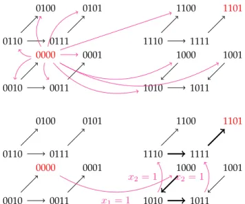
Fig. 1 gives the transition graph of this BN, and the differ-ent perturbation techniques. To understand the benefit of sequential perturbations, let us consider the fixpoint 0000 as starting point and fixpoint 1101 as target.
Obviously, because 0000 is a fixpoint, there can be no sequence of updates from 0000 to 1101. It can also be seen that if one or two vertices are perturbed at the same time, by giving them new values, 1101 is not reachable, as shown in Fig. 1(top). However, if two vertices are perturbed, but the system is allowed to follow its own dynamics between the changes, 1101 can be reached, as shown in Fig. 1(bottom), by using the path 0000−−−→ 1000 → 1010 → 1011x1=1 x2=1
−−−→ 1111 → 1101, i.e. we first force the activation of the first variable, then wait until the system reaches (by its own dynamics) the state 1011 before activating variable 2. From the perturbed state, the system is guaranteed to end up in the desired fixpoint, 1101.
0000 0001 0010 0011 0100 0101 0110 0111 1000 1001 1010 1011 1100 1101 1110 1111 0100 0000 0001 0010 0011 0101 0110 0111 1000 1001 1010 1011 1100 1101 1110 1111 x1= 1 x2= 1 x2= 1
Fig. 1: Transition graph of f and candidate perturbations (magenta) for the reprogramming from 0000 to 1101: (top) none of candidate perturbations of one or two variables in the initial state allow to reach 1101; (bottom) sequences of two sequential perturbations allow to reach 1101.
In this case and almost every other case of sequential reprogramming, the ordering of perturbations is crucial. For example, if the perturbations were done in a different order in this example, the first perturbation to be made would be x2 = 1, then only 0100 would be reachable.
From this state, perturbing with x1 = 1 allows 1100 to be
reachable, and it is the only attractor reachable. 1101 is still unreachable, meaning the perturbations failed to make the target reachable.
Inevitable and existential reprogramming
This example shows that some otherwise unattainable at-tractors may be reached when the changes of values of vertices are coordinated in a particular order, and using the transient dynamics between perturbations. We remark that there exists another reprogramming path, where variable 2 is perturbed when the system reaches 1010. Note that, in this case, after the second perturbation, the system can reach 1101, but it is not guaranteed. We say that, in the first reprogramming path, the reprogramming is inevitable, whereas it is only existential in the second case.
Permanent and temporary perturbations
We also have to consider the sequential characteristics of how individual perturbations act. The system may either only be temporarily perturbed, by changing the value of a vertex i for a time (setting i to 0 or 1), or the change can be permanent, i.e. a modification of the update function of the vertex (setting fi to 0 or 1). On our example, making
permanent changes would yield the solutions given above. However, if the initial state is 1011 and the target state is 1100, then it has different solutions (Fig. 2).
Indeed, if the objective is to go from 1011 to 1100 in the same transition graph using only permanent perturbations, then their order does not matter. Perturbing x2and x4from
1000 1001 1010 1011 1100 1101 1110 1111 1000 1001 1010 1011 1100 1101 1110 1111 \ x2= 1 ; x4= 0 x2= 1 x4= 0
Fig. 2: Right part of the transition graph of f from initial state 1011 to 1100, with permanent perturbations (left) and temporary ones (right).
the initial state is enough to make 1100 the only reachable state. On the other hand, if the perturbations are temporary, x2 has to be perturbed first, then when 1101 is reached,
x4 can be perturbed. If this order is not followed, 1101 is
reachable as well as 1100.
In most cases, the perturbations done in permanent reprogramming and the ones done in temporary reprogram-ming can be on different variables.
3
C
HARACTERIZATIONS OFR
EPROGRAMMINGS
TRATEGIESThis section brings a formal definition of dynamical models adding perturbations to BN dynamics, and the character-ization of sequential reprogramming. It also explains an algorithm to find all inevitable reprogramming solutions, given a maximum number of perturbations k, and applies the algorithm to the example from Sect. 2.
3.1 Perturbed model
Given a BN, perturbations can be added by allowing the variables to change value (temporary or permanently). We introduce the notion of Perturbed Transition Graph (Def. 5) which encompasses the transitions allowed by the BN and transitions due to perturbations. Moreover, a variable vk
tracks the number of applied perturbations. It should be noted that how the perturbations are made, which vari-ables can be perturbed, in which states the varivari-ables can be perturbed, and other details are all part of the model. The model is an input from the user, and should conform to the following definition in order for the properties and algorithm to work on it. An example of perturbed transition graph to model temporary perturbations is given in Sect. 4.
Definition 5 (Perturbed Transition Graph). Given a BN f of dimension n, its transition graph STG(f )=(S, Ef), and a
maximum number of allowed perturbations k, the Perturbed Transition Graph G is a pair (Sp, Ep) where
• Sp= S × [0, k] is the set of states, S is the set of states of
the transition graph with states possibly added to account for the perturbations, times a perturbation counter vk
ranging from 0 to k;
• Ep ⊆ {(s, i) → (s0, i) | i ∈ [0, k], (s → s0) ∈ Ef} ∪
{(s, i) → (s0, i + 1) | i ∈ [0, k − 1], s, s0 ∈ S}, is
4
asynchronous transitions of STG(f) and for perturbations (which increase the perturbation counter by one). Graph layers and layer subsets
The transition graph can be layered by regrouping all states having the same perturbation count in the same layer. Let Nj = Vp× {j} be the set of all states in layer j. A subset
A ⊆ Sprestricted to a layer j is denoted Aj := A ∩ Nj. A
subset A ⊆ Vpof ST G(f ) times a layer j is Aj:= A × {j}.
Property 1. Given a Perturbed Transition Graph G of a BN f
with temporary perturbations, for all i ≤ k, the subgraph Ni
of G is isomorphic to ST G(f ), the original network’s transition graph.
Property 2. If i > j, then (s, j) ∈ Spcannot be reached from
(s0, i) ∈ Sp, regardless of s and s0. That is, the perturbation
counter can only increase.
From the definition of basin (Def. 4), the basin of a set of nodes X restricted to a layer considers only the transitions in the layer.
Definition 6 (Basin restricted to a layer). The basin of X restricted to a layer j, denoted by basj(X), is the biggest set Y
such that X ⊆ Y ⊆ Nj and ∀y ∈ Y \ X, (post(y) ∩ Nj) ⊆
Y ∧ ∃x ∈ X, y →∗x.
3.2 Set characterization of inevitable reprogramming
Given a Perturbed Transition Graph (Sp, Ep) of a BN f with
a maximum number of perturbations k (temporary or per-manent), let φ ⊆ S be a set of states of the original ST G(f ). States in φ are the targets of the inevitable reprogramming. W is the solution set, the set of all states that have inevitable reprogramming from them to one of the target states.
As a reminder, φjis the set of states in φ in STG(f) which
are in layer j in the perturbed transition graph.
In order to compute W, two other sets ψj and Wj for
each layer are computed. ψj is the set of states in layer j
that need to be reached in order to reach one of the target states in φ. Thus, ψjcontains states of φjand states allowing
one or multiple perturbations to a lower layer, where φ can be reached. Wj is the basin, restricted to the layer j, of ψj.
Hence, Wj is the set of states, in layer j, that reach one of
the states in φ, whether the state is in layer j or not. The sets ψj and Wjare defined as follows:
ψk= {x | x ∈ Nk∧ x ∈ φk}
Wk = bask(ψk)
For j between k − 1 and 0:
ψj= {x | x ∈ Nj∧ (x ∈ φj ∨ x ∈ pre(Wj+1)}
Wj = basj(ψj)
Since ψkexists and is defined, all ψjand Wjare defined.
The set describing the solution is W = ∪j∈[1,k]Wj.
If the initial state s0 is in W, then there exist inevitable
reprogramming solutions, and all reprogramming solutions are in W.
Property 3. By construction, the set of all attractors reachable in
the graph restricted to W is a subset of φ × [0, k]. Algorithm using the state set characterization
Algorithm 1 is given in pseudo-code using the set characterization explained previously. The notations are
the same. A loop invariant is that W corresponds to the set of states from layer j to layer k that have inevitable reprogramming to a state in φ.
The inputs of the algorithm are a Perturbed Transition Graph (Sp, Ep), a set of states φ, an initial state s0, and the
maximal number of perturbations, k.
The first step is to set Wk+1 to the empty set, as there
are no states in layer k + 1 (line 2), and W is the set of all possible solutions, hence W = ∅ at the beginning.
Then, for each layer j, ψj has to be computed. ψj is the
set of states either in φj or being direct predecessors of the
solution states of the lower layer, the layer j + 1. The basin of ψj is then computed. These states are the solution states
of layer j, and are added to the set of all solution states, W. When the computation has reached the first layer, either the initial state is not among the solution states, in which case there is no solution for this reprogramming (line 7), or, if s0 ∈ W0, then the set of states containing all inevitable
reprogramming paths is returned (line 9).
Algorithm 1Inevitable Reprogramming relying on the Set Characterization 1: functionREPROGRAMMING(G, φ, s0, k) 2: Wk+1= ∅. 3: W = ∅ 4: for j = kto 0 do 5: ψj= {x ∈ Nj | x ∈ φj ∨ x ∈ pre(Wj+1)} 6: Wj = basj(ψj) 7: W = WS Wj 8: if s06∈ W0then 9: Return ∅ 10: else 11: Return W
One could be surprised by the definition of ψj: in Wj,
we use the basin of ψj, where the system will always reach
one of the state in ψj, and on the other hand, in ψj, only the
preimage of Wj+1is used. However, in this case, we want to
control the system, meaning the perturbations are chosen by the controller. As a consequence, the controller only needs to choose one perturbation among all possible ones in order to reach Wj+1.
Complexity
Given a transition graph G from a network with n variables, and the possibility of doing up to k perturbations, k × m can be defined as the number of states of G, with m = O(en).
Since the algorithm relies on the exploration of subparts of the graph, and the distance between basins of attraction and other layers, the complexity, both in space and time, will vastly depend on the graph properties.
In the worst case, all ln(m) perturbations from a state in ψjhave to be explored, and all k × m states are in different
ψj. Hence, the worst time complexity is in O(k×m×ln(m)),
or, if we use the size of the network as the entry, O(k × n × en).
As for space complexity, the algorithm returns W, which is the set of explored states mentioned for time complexity, giving the same complexity.
inital state
Layer 0
Layer 1
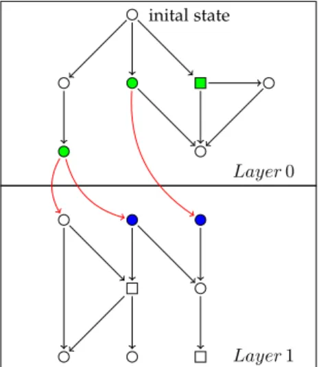
Fig. 3: Computing ψ1, in green.
However, these worst cases happen only if there are only perturbations in the transition graph, meaning there is no inherent dynamics to the model. Typical cases would have a lower time and space complexity.
Visual explanation of the set algorithm
Figures 3 to 7 show an example of the algorithm applied to a transition graph, with the states in φ marked as squares, and perturbation transitions in red. In this example, there are only two layers. Note that each layer of the transition graph should always be the same that layer 0, except for some transitions removed in the case of permanent or durable1
perturbations. Here the two layers are different, it could be a different part of the original transition graph.
Figures 3 and 4 represent the first iteration of the for loop, respectively computing ψ1and then its basin to have
the solution states in the layer 1: W1= bas(ψ1).
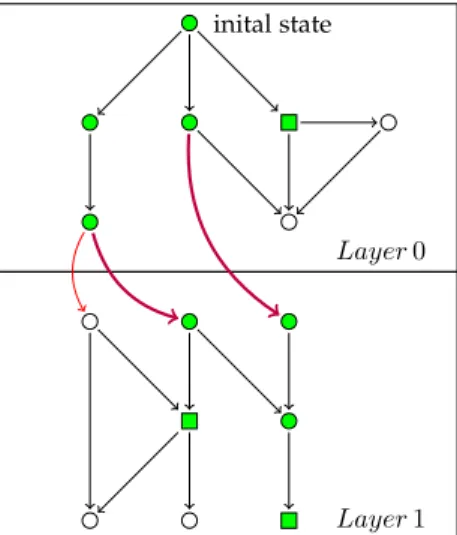
The next two figures, 5 and 6, represent the second itera-tion of the for loop, computing (in green) ψ0, by using some
states in W1(in blue), and then computing W0= bas(ψ0).
Figure 7 represents the last step of the algorithm: since the initial state is in W0, the different perturbations to reach
φ are computed.
The algorithm then returns W, the set of states in green in figure 7. From this set, the perturbations can be extracted using the perturbation counter and by comparing the states. An example on how to do so is given in Sect. 4.
Existential Reprogramming
The algorithm and experiments focus on inevitable repro-gramming as it is the most relevant for applications in cel-lular reprogramming. However, existential reprogramming can be easily achieved with the same algorithm by changing basj(X) to pre∗j(X) on line 6.
As a reminder, in Sect. 2 the definition for pre∗j(X) is the set
of states that can lead to X. This set can then be restricted to states only being in layer j.
Existential Reprogramming is the existence of a path to the 1. One could imagine a model where perturbations change the func-tions of the graph for a given time. In this case, the model and hence the perturbed transition graph are changed.
inital state
Layer 0
Layer 1
Fig. 4: Computing W1= bas(ψ1), in green.
inital state
Layer 0
Layer 1
Fig. 5: In green, ψ0in the layer 0, and in blue the successors
in W1.
inital state
Layer 0
Layer 1
6
inital state
Layer 0
Layer 1
Fig. 7: Marking in green W, and in purple the perturbations possible. 0000,0 0001 1000,1 1010,1 1011,1 1111,2 1101,2 0010 0011 0100 0101 0110 0111 1001 1100 1110 x1= 1 x2= 1
Fig. 8: The perturbation path returned by the algorithm on the example of Sect. 2.
solution. By using the set of predecessors instead of the basin, the algorithm no longer guarantees the reprogram-ming, but still guarantees the target to be reachable with the perturbations returned.
3.3 Example
Applied on the example of Sect. 2 for the inevitable repro-gramming from 0000 to 1101 with k = 2, W is the set of highlighted states, meaning all states not in gray in Fig. 8, and the algorithm returns (x1 = 1, x2 = 1) as the only
solution. The perturbation count is the number after the comma in the state.
The sequential reprogramming path identified in Sect. 2 is the only strategy for inevitable reprogramming.
A more complete explanation is given in sub-sect. 4.3, with the implemented version of the algorithm.
4
C
OMPUTATION OF THE TEMPORARY SEQUEN-TIAL REPROGRAMMING PATHS
In Sect. 3, we have introduced a general algorithm to compute all the inevitable reprogramming solutions for the temporary and the permanent sequential control. In this section, we focus on the temporary sequential control, and we propose an algorithm to find the minimal number of perturbations and the associated reprogramming paths.
4.1 Encoding BNs with temporary perturbations in BDDs
Binary decision diagrams (BDDs) were introduced by Lee in [10] and Akers in [2] to represent Boolean functions [10], [2]. BDDs have the advantage of memory efficiency and have been applied in many model checking algorithms to alleviate the state space explosion problem.
A BN with temporary perturbations, denoted as G(Vp, fp) is constructed by adding a variable vkto V , whose
value denotes the number of perturbations, and adding functions to f to enable the perturbations of the variables V . These functions allow any variable to change value at the cost of increasing the perturbation counter vk. It can
be modeled as a perturbed transition graph G(Sp, Ep) as
described in Sect. 3, which can then be encoded in a BDD. Each variable in Vp can be represented by a BDD variable.
Specifically, the Boolean variables V ∈ Vp are binary BDD
variables and the perturbation counter vk is a bounded
integer variable, whose value is in [0, k]. By slight abuse of notation, we also use Vpto denote the set of BDD variables.
In order to encode the transition relations, another set Vp0
of BDD variables, which is a copy of Vp, is introduced: Vp
encodes the possible current states, i.e., x(t), and Vp0encodes
the possible next states, i.e., x(t + 1).
4.2 Method for the computation of the temporary se-quential reprogramming paths
In Sect. 3, we described Algorithm 1 to compute inevitable reprogramming solutions with k perturbations. In this sec-tion, we modify Algorithm 1 to derive a method to compute the minimal number of perturbations and the corresponding inevitable temporary reprogramming paths in Algorithm 2. As mentioned in Sect. 4.1, we encode BNs with pertur-bations in BDDs, hence most operations of the algorithm are performed with BDDs. This algorithm takes a BN with perturbations G, the maximal number of perturbations al-lowed k, a source attractor Asand a target attractor At as
inputs. Note that At is an attractor of the original STG(f )
and does not contain the value of the perturbation counter. If there exist temporary reprogramming paths within k perturbations, the minimal number of perturbations pmin
and all inevitable temporary reprogramming paths ρ will be returned as outputs.
We first compute the corresponding set of states of the target attractor Atin the perturbed transition graph at each layer i, i ∈ [0, k] as line 3. We cycle through lines 4–15 to compute the minimal number of perturbations pminand the
corresponding reprogramming paths ρ. Let m denote the number of perturbations. Starting from m = 0, we gradually increase m by 1 until we find a solution or m is greater than k. For each m, we compute two sets W and P according to lines 6-9. Wm is the basin of the projection of the target
attractor at layer m (line 6). Pi, i ∈ [0, m − 1] stores the
direct predecessors of Wi+1at layer i and Wi, i ∈ [0, m − 1]
is the basin of Piat layer i. The basin is computed using the
fixed point computation of strong basins in [16]. In this way, any state s, s ∈ Pican reach a state s0, s0 ∈ Wi+1with one
perturbation and any state s, s ∈ (Wi\ Pi) can reach a state
Algorithm 2Temporary sequential reprogramming of BNs
1: procedureCOMPUTATION OF SEQUENTIAL REPROGRAMMING PATHS(G, As, At, k)
2: Initialize the minimal number of perturbation pmin= 0, flag = False;
3: Compute the corresponding set of states of A at each layer i, i ∈ [0, k], denoted as {At0, At1, . . . , Atk}.
4: for m = 0; m <= k; m + + do
5: Initialize W = {W0, W1, . . . , Wm}, P = {P0, P1, . . . , Pm−1};
6: Wm= basm(Atm)
7: for z = m − 1; z >= 0; z − − do
8: Pz= pre(Wz+1) ∩ Nz
9: Wz = basz(Pz) ∩ Nz // local basin of Pzat layer z
10: if As⊆ W0then
11: pmin= m, flag = True
12: Initialize a vector ρ to store the paths.
13: ρ =COMPUTE PATHS(1, As, ρ, W, P); // Algorithm 3
14: TSρ = EXTRACT PATHS(ρ, TS ).
15: break;
16: if flag == False then
17: There is no temporary sequential reprogramming paths within k perturbations.
Algorithm 3Helper functions
1: procedureCOMPUTE PATHS(z, Tz−1, ρ, W, P)
2: Sz= post∗(Tz−1) ∩ Pz−1; 3: Tz= post(Iz) ∩ Wz; 4: Insert (Sz, Tz) to ρ. 5: if z < W.size() then 6: ρ =COMPUTE PATHS(z + 1, Tz, ρ, W, P) 7: return ρ
8: procedureEXTRACT PATHS(ρ, TS ) 9: Initialize a BDD TSρ
10: for (Sz, Tz) ∈ ρ, z ∈ [1, m] do
11: Add the transition relation from any state s in Sz
to any state t in Tzto TSρ.
TSρ= TSρ∧ TS
12: return TSρ
For the two loops, an invariant is that m is the maximum number of perturbations for a minimal solution. The first loop stops when such a m is found, and the fact that W is the set of states that have an inevitable reprogramming solution to A, as in Algorithm 1.
There exist reprogramming paths with m perturbations if and only if As ⊆ W
0. If so, the minimum number of
perturbations required is m and the reprogramming paths ρ can be computed with Procedure “COMPUTE PATHS” in Algorithm 3. We start with Asand by iteratively performing
lines 2-4 of Algorithm 3, we can identify all the paths ρ from s to A with m perturbations. ρ stores a list of tuples {(S1, T1), (S2, T2) . . . , (Sm, Tm)}. S1 is a set of states at
layer 0, that can be reached by the source state s0
spon-taneously. With one perturbation, any state s1, s1 ∈ S1
can reach a state t1, t1 ∈ T1, and t1 can always reach a
state s2, s2 ∈ S2. With the co-action of the spontaneous
evolutions of BNs and m perturbations, the network will eventually reach At.
However, Szand Tz, z ∈ [1, m] are two sets of states, for
any state sz∈ Sz, its successors post(sz) are a subset of Tz
and this information is missing in ρ. In order to identify the
reprogramming determinants, we extracted the transition relations of the reprogramming paths T Sρfrom the
transi-tion system T S using Procedure “EXTRACT PATHS” . Due to the utilization of the spontaneous evolutions of BNs, this method requires a full observation of the transition system to identify which path the system follows.
Existential Reprogramming
As for Algorithm 1, Existential Reprogramming can be achieved easily by replacing basz(X) by pre∗z(X) in
Algo-rithm 2.
4.3 Example
For the example in Sect. 2, we compute all the minimal inevitable sequential reprogramming paths from 0000 to 1101 with Algorithm 2. We cycle through lines 4-15 and increase the number of perturbations m from 0 to k until we find a solution. Fig. 9 shows the computation process when m = 2. For every state, the number after the comma is the perturbation count. We first compute W and P according to lines 6-9. At layer 2, W2 (green and red states) is the basin
of the projection of the target at that layer, 1101,2. At layer 1, P1(green states) represents the predecessors of W2, from
which, by applying one perturbation, we can each one of the state in W2. And W1(green and blue states) is the basin
of P1at layer 1. Similarly, P0represents the predecessors of
W1and W0is the basin of P0at layer 0. For this example, P0
and W0are the same, and they include green and red states
at layer 0. Since the source state 0000,0 is in W0, the minimal
number of perturbation required is 2.
We compute the reprogramming paths by iteratively applying the procedure COMPUTE PATHS. The intersection S1 = {0000,0} of P0with the successors of the source state
0000,0 at layer 0, is the set of states from which we can apply one perturbation to reach a subset T1 = {1000,1} of W1.
The intersection S2= {1011,1} of P1with the successors of
T1 at layer 1, is the set of states from which we apply the
second perturbation to reach a subset T2 = {1111,2}
8
{(S1:{0000,1}, T1:{1000,1}), (S2:{1011,1}, T2:{1111,2})}.
For this example, there is only one path and the repro-gramming determinants are x1 and x2. The whole control
process will be s0→ S1 x1=1 −−−→ T1→ S2 x2=1 −−−→ T2→ A2. 0101,0 0111,0 0110,0 0100,0 1100,0 1110,0 1111,0 1101,0 0001,0 0011,0 0010,0 0000,0 1000,0 1010,0 1011,0 1001,0 Layer 0 0101,1 0111,1 0110,1 0100,1 1100,1 1110,1 1111,1 1101,1 0001,1 0011,1 0010,1 0000,1 1000,1 1010,1 1011,1 1001,1 Layer 1 0101,2 0111,2 0110,2 0100,2 1100,2 1110,2 1111,2 1101,2 0001,2 0011,2 0010,2 0000,2 1000,2 1010,2 1011,2 1001,2 Layer 2 x1= 1 x2= 1
Fig. 9: Computation of reprogramming paths of the example of Sect. 2 with Algorithm 2.
5
C
ASE STUDIESTo demonstrate the efficiency and effectiveness of the tem-porary sequential control method, we apply it to three real-life biological networks. The method is implemented in ASSA-PBN[13], based on the model checker MCMAS [11] to encode BNs into BDDs. All the experiments are performed on a computer (MacBook Pro), which has a CPU of Intel Core i7 @3.1 GHz and 8 GB of DDR3 RAM. Program executables and model files are provided as supplementary material. We first describe the three biological networks.
The cardiac gene regulatory networkis constructed for the early cardiac gene regulatory network of the mouse, includ-ing the core genes required for the cardiac development and the FHF/SHF determination [9]. This network has 15 variables and 6 single-state attractors.
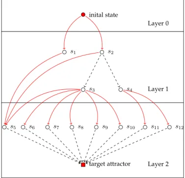
inital state s1 s2 s3 s4 s5 s6 s7 s8 s9 s10 s11 s12 target attractor Layer 0 Layer 1 Layer 2
Fig. 10: Reprogramming paths from attractor A2to attractor
A5for the cardiac network.
The PC12 cell differentiation networkis a comprehensive model used to clarify the cellular decisions towards pro-liferation or differentiation [15]. It shows the interactions between protein signalling, transcription factor activity and gene regulatory feedback in the regulation of PC12 cell differentiation after the stimulation of NGF. This network consists of 32 variables and has 7 single-state attractors.
The bladder networkis designed for studying patterns and conceiving counter-intuitive observations, which allow us to formulate predictions about conditions where combining genetic alterations benefits tumorigenesis [17]. This network consists of 35 variables. It has 5 single-state attractors and 3 cyclic attractors.
We choose two different attractors as the source and target attractors. For each pair of the source and target at-tractors, we compute the minimal number of perturbations and all inevitable reprogramming paths for the sequential control.
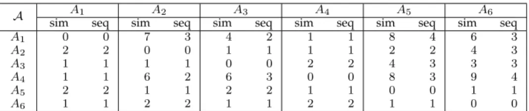
Table 1, 2 and 3 give the minimal number of perturba-tions for the initial reprogramming [16] and the sequential control on three networks for all combinations of the source and the target attractors. It is obvious that the sequential control always outperforms the initial reprogramming in terms of the number of perturbations. This is due to the fact that the initial reprogramming performs all the per-turbations at once [16], while our sequential control takes advantage of the spontaneous evolutions of the networks, which helps to drive the network towards the desired target. We compute all possible inevitable paths for every pair of the source and the target attractors. Figure 10 describes the reprogramming paths from attractor A2 to attractor A5
for the cardiac network. It is also a partial transition system of the cardiac network with perturbations. The red arrows represent perturbations and the dashed arrows represent
A A1 A2 A3 A4 A5 A6
sim seq sim seq sim seq sim seq sim seq sim seq
A1 0 0 7 3 4 2 1 1 8 4 6 3 A2 2 2 0 0 1 1 1 1 2 2 4 3 A3 1 1 1 1 0 0 2 2 4 3 3 3 A4 1 1 6 2 6 3 0 0 8 3 9 4 A5 2 2 1 1 2 2 1 1 0 0 1 1 A6 1 1 2 2 1 1 2 2 1 1 0 0
TABLE 1: The minimal number of perturbations for the initial reprogramming and the sequential control on the cardiac network.
A A1 A2 A3 A4 A5 A6 A7
sim seq sim seq sim seq sim seq sim seq sim seq sim seq
A1 0 0 1 1 10 2 1 1 11 3 2 2 1 1 A2 9 8 0 0 1 1 10 9 3 2 11 10 10 9 A3 7 7 1 1 0 0 8 8 1 1 9 9 8 8 A4 1 1 1 1 10 2 0 0 11 3 1 1 2 2 A5 8 8 1 1 1 1 9 9 0 0 8 8 7 7 A6 2 2 1 1 11 2 1 1 10 3 0 0 1 1 A7 1 1 1 1 11 2 2 2 10 3 1 1 0 0
TABLE 2: The minimal number of perturbations for the initial reprogramming and the sequential control on the PC12 cell network.
A A1 A2 A3 A4 A5 A6 A7 A8
sim seq sim seq sim seq sim seq sim seq sim seq sim seq sim seq
A1 0 0 1 1 1 1 3 3 2 2 2 2 7 4 13 4 A2 1 1 0 0 2 2 8 4 1 1 9 3 10 3 8 3 A3 1 1 2 2 0 0 2 2 1 1 3 3 3 3 7 3 A4 3 3 2 2 2 2 0 0 3 3 1 1 1 1 9 3 A5 2 2 1 1 1 1 3 3 0 0 8 4 2 2 4 2 A6 2 2 1 1 3 3 1 1 4 2 0 0 6 2 14 4 A7 4 2 1 1 3 3 1 1 2 2 6 2 0 0 6 2 A8 2 2 1 1 1 1 6 3 2 2 12 4 5 4 0 0
TABLE 3: The minimal number of perturbations for the initial reprogramming and the sequential control on the bladder network. T(s) A1 A2 A3 A4 A5 A6 A1 0 0.115 0.082 0.007 0.186 0.171 A2 0.013 0 0.045 0.006 0.1 0.166 A3 0.005 0.045 0 0.012 0.133 0.196 A4 0.007 0.069 0.099 0 0.134 0.228 A5 0.011 0.044 0.072 0.006 0 0.043 A6 0.007 0.069 0.067 0.012 0.063 0
TABLE 4: The time costs of the sequential control on the cardiac network. T(s) A1 A2 A3 A4 A5 A6 A7 A1 0 0.188 0.463 0.479 0.458 0.473 0.486 A2 3.509 0 0.446 3.803 0.254 2.676 4.358 A3 2.906 0.185 0 3.843 0.21 2.86 3.597 A4 0.833 0.188 0.467 0 0.457 0.399 0.519 A5 3.589 0.183 0.4 5.792 0 3.473 3.229 A6 0.946 0.188 0.453 0.485 0.542 0 0.43 A7 1.183 0.189 0.453 0.601 0.545 0.388 0
TABLE 5: The time costs of the sequential control on the PC12 cell network. T(s) A1 A2 A3 A4 A5 A6 A7 A8 A1 0 1.037 3.909 2.984 15.547 3.519 7.318 5.991 A2 3.37 0 6.11 12.349 6.64 10.705 5.286 4.651 A3 3.538 1.073 0 2.402 6.559 3.249 5.467 4.581 A4 5.426 1.073 6.085 0 18.906 1.737 0.951 4.564 A5 3.987 0.995 3.908 3.277 0 43.301 4.238 3.344 A6 4.037 0.982 9.357 2.325 16.124 0 4.273 9.803 A7 4.144 0.991 6.882 1.974 16.021 4.974 0 3.340 A8 4.13 0.973 4.659 3.107 16.106 11.763 8.111 0
TABLE 6: The time costs of the sequential control on the bladder network.
paths in the transition system. The initial state is A2at layer
0 and the target attractor is the extension of A5 at layer 2.
By perturbing variables “Tbx5” or “Nkx25”, we can reach s1or s2at layer 1. At this step, on one hand, we can perturb
“Nkx25” at s1 or “Tbx5” at s2 to reach s5 at layer 2. On
the other hand, we can let the network evolve and when the network is at states s3 or s4, by performing different
perturbations, we can reach one of the states (s5-s12) at layer
2, which is in the basin of the target attractor A5at layer 2.
In this way, the network will eventually reach the target attractor spontaneously.
Table 4, 5 and 6 show the time costs of the sequential control on three networks. The time costs include the com-putation of the minimal number of perturbations as well as the computation of all inevitable reprogramming paths. The ranges of the time costs for the cardiac network, the PC12 network and the bladder network are 0.005-0.228, 0.183-5.792, 0.951-43.301 seconds, indicating the efficiency and scalability of our sequential control method. There are mainly two factors that influence the efficiency of the se-quential control: the minimal number of perturbations and the number of reprogramming paths. If the required mini-mal number of perturbations is big, many iterations will be performed since we start from m = 0. Meanwhile, it also takes time to compute all the solutions using the procedure “COMPUTE PATHS” if there exist many reprogramming paths.
10
6
D
ISCUSSIONSequential reprogramming consists in applying perturba-tions in a specific order and in specific states of the system to trigger and control an attractor change. It relies on the tran-sient dynamics of the system. Sequential reprogramming is interesting for biologists wanting to reprogram cells: it can return new targets, and can lower costs by requiring lighter interventions.
As discussed in Sect. 2, initial reprogramming is only allowing perturbations from the initial state, thus there is no order needed. This case is discussed in multiple other works, and has been the main computation technique for perturbations. Once all the perturbations have been done, the system stabilizes itself in the targeted attractor. By ordering and “waiting” between the perturbations, other dynamics of the system can be used, thus possibly reducing the number of variables to be perturbed, and returning new solutions.
Other works [4], [8], [3], [19] can use probabilistic meth-ods to determine perturbations to do in the initial state. These reprogramming techniques compute initial existential reprogramming. Technically, no proof is given that the net-work will reach the wanted target, however there is a high probability that it will. Some of these works [4], [3] choose an initial state randomly for each test.
Some works [5], [20] focus on making the target always reached, but still only use initial perturbations, making them initial inevitable reprogramming techniques.
In other works [1], [18], the model allows for sequential reprogramming, making them sequential existential repro-gramming. In [1], the existence of solutions is checked through a model checker, and specific perturbation paths can be tested. In [18], the model is probabilistic and use time-series data, thus allowing to make perturbations at different times in the series.
Lastly, some works [23], [12] allow for sequential in-evitable reprogramming.
Most of mentioned methods provide incomplete or non-guaranteed results. Our aim is to provide a formal frame-work for the complete and exact characterization of the initial state and sequential reprogramming of Boolean net-works.
This paper establishes a set characterization of sequen-tial reprogramming for Boolean networks with either per-manent (mutations) or temporary (e.g, through signalling) perturbations. Perturbations can be applied at the initial state, and during the transient dynamics of the system. This later feature allows identifying new strategies to reprogram regulatory networks, by providing solutions with different targets and possibly requiring fewer perturbations than when applied only in the initial state.
The algorithm we designed relies on modelling the com-bination of Boolean network asynchronous transitions with perturbation transitions by using binary decision diagrams. The identification of sequential reprogramming solutions then relies on an explicit exploration of the resulting tran-sition system. Our method has no restriction on the nature of the target state, which could be either a transient state, fixed point attractor, or within a cyclic attractor. Our frame-work can handle temporary perturbations for the inevitable
reprogramming to the targeted state, and the use of BDDs allows for some scalability as supported by performed case studies.
A
CKNOWLEDGMENTSThis research was supported by the ANR-FNR project “AlgoReCell” (ANR-16-CE12-0034; FNR INTER/ANR/15/11191283); Labex DigiCosme (project ANR-11-LABEX-0045-DIGICOSME) operated by ANR as part of the program “Investissement d’Avenir” Idex Paris-Saclay (ANR-11-IDEX-0003-02); CNRS PEPS INS2I 2017 “FoRCe”; and by the project “SEC-PBN” funded by University of Luxembourg.
R
EFERENCES[1] W. Abou-Jaoud´e, P. T. Monteiro, A. Naldi, M. Grandclaudon, V. Soumelis, C. Chaouiya, and D. Thieffry. Model checking to assess T-helper cell plasticity. Frontiers in Bioengineering and Biotechnology, 2, 2015.
[2] S. B. Akers. Binary decision diagrams. IEEE Transactions on Computers, 100(6):509–516, 1978.
[3] R. Chang, R. Shoemaker, and W. Wang. Systematic search for recipes to generate induced pluripotent stem cells. PLoS Computa-tional Biology, 7(12):e1002300, Dec 2011.
[4] D. P. A. Cohen, L. Martignetti, S. Robine, E. Barillot, A. Zinovyev, and L. Calzone. Mathematical modelling of molecular pathways enabling tumour cell invasion and migration. PLOS Computational Biology, 11(11):1–29, 11 2015.
[5] I. Crespo, T. M. Perumal, W. Jurkowski, and A. del Sol. Detecting cellular reprogramming determinants by differential stability anal-ysis of gene regulatory networks. BMC Systems Biology, 7(1):140, 2013.
[6] A. del Sol and N. J. Buckley. Concise review: A population shift view of cellular reprogramming. STEM CELLS, 32(6):1367–1372, 2014.
[7] T. Graf and T. Enver. Forcing cells to change lineages. Nature, 462(7273):587–594, dec 2009.
[8] R. Hannam, A. Annibale, and R. Kuehn. Cell reprogramming modelled as transitions in a hierarchy of cell cycles. ArXiv e-prints, Dec. 2016.
[9] F. Herrmann, A. Groß, D. Zhou, H. A. Kestler, and M. K ¨uhl. A boolean model of the cardiac gene regulatory network determin-ing first and second heart field identity. PLOS ONE, 7(10):1–10, 10 2012.
[10] C.-Y. Lee. Representation of switching circuits by binary-decision programs. Bell System Technical Journal, 38(4):985–999, 1959. [11] A. Lomuscio, H. Qu, and F. Raimondi. MCMAS: an open-source
model checker for the verification of multi-agent systems. Inter-national Journal on Software Tools for Technology Transfer, 19(1):9–30, 2017.
[12] H. Mandon, S. Haar, and L. Paulev´e. Temporal Reprogramming of Boolean Networks. In CMSB 2017 - 15th conference on Com-putational Methods for Systems Biology, volume 10545 of Lecture Notes in Computer Science, pages 179–195. Springer International Publishing, 2017.
[13] A. Mizera, J. Pang, C. Su, and Q. Yuan. ASSA-PBN: A toolbox for probabilistic boolean networks. IEEE/ACM Transactions on Computational Biology and Bioinformatics, 15(4):1203–1216, 2018. [14] M. K. Morris, J. Saez-Rodriguez, P. K. Sorger, and D. A.
Lauf-fenburger. Logic-based models for the analysis of cell signaling networks. Biochemistry, 49(15):3216–3224, 2010. PMID: 20225868. [15] B. Offermann, S. Knauer, A. Singh, M. L. Fern´andez-Cach ´on,
M. Klose, S. Kowar, H. Busch, and M. Boerries. Boolean modeling reveals the necessity of transcriptional regulation for bistability in PC12 cell differentiation. F. Genetics, 7:44, 2016.
[16] S. Paul, C. Su, J. Pang, and A. Mizera. A decomposition-based approach towards the control of Boolean networks. In Proc. 9th ACM Conference on Bioinformatics, Computational Biology, and Health Informatics. ACM, 2018.
[17] E. Remy, S. Rebouissou, C. Chaouiya, A. Zinovyev, F. Radvanyi, and L. Calzone. A modelling approach to explain mutually exclu-sive and co-occurring genetic alterations in bladder tumorigenesis. Cancer research, pages canres–0602, 2015.
[18] S. Ronquist, G. Patterson, M. Brown, H. Chen, A. Bloch, L. Muir, R. Brockett, and I. Rajapakse. An Algorithm for Cellular Repro-gramming. ArXiv e-prints, Mar. 2017.
[19] O. Sahin, H. Frohlich, C. Lobke, U. Korf, S. Burmester, M. Ma-jety, J. Mattern, I. Schupp, C. Chaouiya, D. Thieffry, A. Poustka, S. Wiemann, T. Beissbarth, and D. Arlt. Modeling ERBB receptor-regulated G1/S transition to find novel targets for de novo trastuzumab resistance. BMC Systems Biology, 3(1):1–20, 2009. [20] R. Samaga, A. Von Kamp, and S. Klamt. Computing combinatorial
intervention strategies and failure modes in signaling networks. Journal of Computational Biology, 17(1):39–53, Jan 2010.
[21] K. Takahashi and S. Yamanaka. A decade of transcription factor-mediated reprogramming to pluripotency. Nat Rev Mol Cell Biol, 17(3):183–193, Feb 2016.
[22] R.-S. Wang, A. Saadatpour, and R. Albert. Boolean modeling in systems biology: an overview of methodology and applications. Physical Biology, 9(5):055001, 2012.
[23] J. G. T. Za ˜nudo and R. Albert. Cell fate reprogramming by control of intracellular network dynamics. PLOS Computational Biology, 11(4):1–24, 04 2015.