HAL Id: hal-03034555
https://hal.archives-ouvertes.fr/hal-03034555
Submitted on 1 Dec 2020
HAL is a multi-disciplinary open access
archive for the deposit and dissemination of
sci-entific research documents, whether they are
pub-lished or not. The documents may come from
teaching and research institutions in France or
abroad, or from public or private research centers.
L’archive ouverte pluridisciplinaire HAL, est
destinée au dépôt et à la diffusion de documents
scientifiques de niveau recherche, publiés ou non,
émanant des établissements d’enseignement et de
recherche français ou étrangers, des laboratoires
publics ou privés.
Modelling charge generation and transport in solid
organic dielectrics under DC stress
Séverine Le Roy, Thi Thu Nga Vu, Christian Laurent, G. Teyssedre
To cite this version:
Séverine Le Roy, Thi Thu Nga Vu, Christian Laurent, G. Teyssedre. Modelling charge generation
and transport in solid organic dielectrics under DC stress. European Seminar on Materials for HVDC
Cables and Accessories: Performance, Modelling, Testing, Qualification (Jicable-HVDC), Perpignan,
France, 18-20 Nov. 2013, Nov 2013, Perpignan, France. pp. 1-5. �hal-03034555�
Modelling charge generation and transport in solid organic dielectrics
under DC stress
Séverine LE ROY, Thi Thu Nga VU, Christian LAURENT, Gilbert TEYSSEDRE; LAPLACE – Laboratoire Plasma et Conversion d'Energie - Université P Sabatier, Bat 3R3, 118 Route de Narbonne, 31062 Toulouse, (France)
[email protected], [email protected], [email protected],
ABSTRACT
Models describing the behavior of organic dielectric under electrical and thermal stress would be extremely useful in the development of more compact, reliable and eco-friendly systems for conversion and transport of electric energy. With information on conductivity and permittivity, it is possible to predict the behavior of a dielectric as a function of temperature and field. These data are however not sufficient and space charges need to be taken into account. Hence, models including charge generation and transport function of time and space need to be developed. It is particularly the case when the object under study is a cable, as the electric field and temperature are no more homogeneous within the insulation. In the present paper, simulations have been performed using a one-dimensional cylindrical model, featuring charge injection, transport, trapping, detrapping and recombination, in order to highlight the effects of geometry, temperature and temperature gradients on the material behavior.
KEYWORDS
Model, space charge, transport, plane parallel geometry, cable geometry, mobility, hopping, temperature and field dependent phenomena.
INTRODUCTION
Challenges in the field of solid insulating materials are linked to the development of more compact, reliable and eco-friendly systems for conversion and transport of electric energy. Polyethylene has advantageously replaced oil-impregnated paper as insulation in high voltage AC cables, and is now the favorite insulating material for HVDC technologies for electrical energy transport. HVDC cables are used in critical applications such as long distance transmissions, interconnexion of asynchronous networks, power link for isolated regions (islands, offshore platforms). For these large-scale electrical networks, the reliability needs to be maximal. It is however well known that space charge may build up in the bulk of the insulation under various temperatures and electric fields, due to charge injection at electrodes or to dissociation of residues and impurities inside the bulk. These charges may affect the reliability of the dielectric, by enhancement of the electric field as an example. The presence of cable joints, and hence interfaces between insulating materials having different electrical properties is also likely to favor charge accumulation at the interfaces. Hence, the presence of charges remains the major problem in the increase of reliability of such electrical systems. Models would be extremely useful to predict the material behavior, and to answer to the main industrial issues. The easiest way to simulate the insulating material behavior is to model its macroscopic behavior with the
help of its conductivity, which is function of temperature and field. This kind of model, based on conductivity measurements, is really useful, as it is able to describe the space charge accumulation at an interface between two materials having conductivities and permittivities that vary differently with temperature and field [1,2]. The simulated results using such models are consistent when compared to accumulated space charge measured on plane parallel samples [2]. However, the simulated results deviate from the experimental space charge behavior when considering cable geometry and taking into account the real temperature gradient inside the dielectric [3]. This could be due to the fact that processes such as charge generation and conduction are not taken into account. Hence, more complex models also need to be developed, that take into account charge generation and transport mechanisms. These models generally consider the generation of charges at the electrodes, transport and trapping inside the bulk and recombination. They are one dimensional, function of the thickness of the plane parallel sample, and time dependent. Only few attempts have been made to develop these transport models for cable geometry [4]. This work focuses on modeling the material electrical behavior in a cylindrical configuration, and to investigate the evolution of measurable variables such as space charge with temperature and field gradient, which are present in a cable system.
CHARGE TRANSPORT MODEL
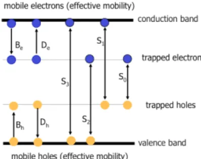
The physical model is based on the scheme represented in Figure 1 [5]. Electronic carriers are provided by injection at the electrodes. Conduction takes place via a hoping mobility, traducing the transport of carriers through shallow levels that are related to the structural disorder of the polymer. Deep trapping is described using a unique level of deep traps for each kind of carriers, from where charges can escape by thermal activation.
Figure 1: Schematic representation of the charge transport model.
Recombination processes involving mobile and trapped carriers are taken into account. For sake of simplification, internal charge generation (dissociation) is not included in the model.
Under service conditions, the Laplacien field inside the dielectric is not uniform, due to the cylindrical geometry. Moreover, the current flowing in the conductor produces an increase in the temperature at the vicinity of the inner electrode, leading to a non-uniformity of the temperature inside the dielectric. Figure 2 shows an example of field and temperature distribution in a 1.5 mm cable (mini-cable) submitted to an applied field of 40 kV/mm, where the inner temperature is at 60°C, whereas the outer electrode is at 20°C (the geometry will have a non negligible effect on the mechanisms taken into account in the simulations).
Figure 2: temperature and field dependence upon the cylindrical geometry
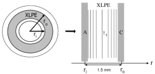
A schematic representation of the cylindrical system used for the discretization of the dielectric is given in Figure 3. Based on this representation, the time and space dependent equations describing the behaviour of charge carriers in cylindrical geometry are the following, neglecting diffusion: ) , ( ) , ( 1 ) , ( t r s r t r j r t t r n a a a = ∂ ∂ + ∂ ∂ (1) ε ρ( , ) ) , ( 1 r t r t r V r r r =− ∂ ∂ ∂ ∂ (2) ) , ( ). , ( ). , ( ) , (rt rt n rt E rt ja =µa a (3)
where na represents the carrier density (electrons and
holes, trapped or mobiles), t is the time, r is the radius. ja
is the current density referring to the mobile carriers, and sa(r,t) is the source term, representing all the mechanisms
inducing a variation of space charge, and not linked to transport. V is the voltage, ρ is the net charge density, ε is the permittivity. µa is the mobility of the mobile carrier, and
E is the electric field.
Transport is described using a hoping type mobility of the form, for each carrier:
= ) ( 2 ) , ( sinh ) ( exp ) , ( 2 ) , ( , , r T k d t r eE r T k ew t r E d t r B B h e h eµ µ ν µ (4)
where d is the distance between traps, and e the elementary charge. ν is the attempt to escape frequency,
Im p ossib le d'affi cher l'im age. Vot r e or d in ateur m an que peut- êtr e de m ém o ir e p our ouvr ir l'im age ou l'i m age es t en dom m agée. Redém ar r ez l 'o r din at eu r , pui s ouv rez à n ou veau le fi ch ier . Si le x r o uge est to ujo ur s affi ché, vo us devr ez peut - êtr e sup pr im er l'im age avant de la réin sér er . XLPE
r i
r o
Im p ossib le d'affi cher l'im age. Vot r e or d in ateur m an que peut- êtr e de m ém o ir e p our ouvr ir l'im age ou l'i m age es t en dom m agée. Redém ar r ez l 'o r din at eu r , pui s ouv rez à n ou veau le fi ch ier . Si le x r o uge est to ujo ur s affi ché, vo us devr ez peut - êtr e sup pr im er l'im age avant de la réin sér er . XLPE r i r o XLPE r i r o XLPE A C ri 1.5 mm ro r !1 Figure 3: schematic representation of the one-dimensional cylindrical system used in the
simulations.
kB the Boltzmann constant, wµe and wµh the hopping
barrier height for electrons and holes respectively. T is the temperature, function of the radius.
Deep trapping is described through a single trapping level for each kind of carrier. Charge carriers have a given probability to escape from traps by overcoming a potential barrier, wtr. This is accounted for by the detrapping
coefficients Di of the form:
− = ) ( exp . ) , ( , , r T k ew t r D B trh tre h e ν (5)
The recombination of carriers is accounted for considering different coefficients Si for the several electron-hole pairs.
The only source of charges is the injection of electronic carriers at each electrode, which is function of the sign of the electric field at the electrode. Prior to electric field application, we consider that the Fermi level of the metal has the same energy value as the Fermi level of the dielectric, i.e. that both materials are in thermodynamic equilibrium. This means that prior to electric field application, there is a current flowing from the metal towards the dielectric, counterbalanced by a current flowing from the dielectric towards the metal. When the electric field is applied, this ‘reverse current’ is still present, even if the net current is clearly directed towards the dielectric. In order to include this mechanism in the modeling, a modified Schottky law has been used for charge injection at each electrode, of the form:
− − = 1 4 ) , ( ) ( exp ) ( exp ) ( ) , ( 0 , 2 , r B B h e h e t r eE r T k e r T k ew r AT t r j ε πε (6)
where r=ri for the anode and r=ro for the cathode.It should
be noted that there is no extraction barrier at the electrodes, so the extraction fluxes for holes at the cathode and for electrons at the anode follow the transport equation.
In the modeling, the temperature distribution is of the form:
(
)
− − = i o o i i i r r r T r T r r r T r T ln ) ( ) ( ln ) ( ) ( (7)where T(ri) and T(ro) are the temperature at the inner and
RESULTS AND DICUSSION
In this section, simulations have been performed on a cable, the inner radius (ri) being 1.9 mm, the outer radius
(ro) being 3.4 mm, providing an insulation thickness of 1.5
mm. Note that the anode is the inner electrode, and the cathode is the outer electrode. Hence, a positive voltage of 60 kV is applied at the inner electrode. The parameters used for the simulations are given in Table 1, and are the ones that have been optimized from measurements
achieved on space charge, current and
electroluminescence, for a plane parallel LDPE [5].
Geometry dependence
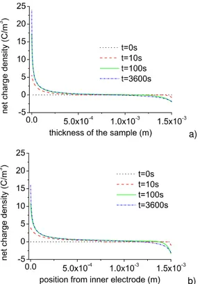
Figure 4 compares the simulated net charge density at the beginning and after one hour of polarization, for a plane parallel geometry [5] and a cylindrical geometry, at 60°C, for the parameters listed in Table 1. Note that the influence charges (capacitive + image charges) have not been added to the simulated profiles in order to better compare the different results. After voltage application (10s), positive charges are detected at the vicinity of the anode in the plane parallel geometry, whereas positive charges have already penetrated deep inside the material for the cylindrical geometry.
Negative charges have also been injected at the cathode side for both cases, and remain at the vicinity of the electrode. After one hour of polarization, the plane parallel sample shows positive charges in the first half of the dielectric, and negative charges in the second half, these charges being considered as homocharges. Positive homocharges, enhanced by the electric field non-uniformity, dominate the space charge profile for the cylindrical geometry at the end of the polarization. Negative homochages injected at the cathode are observed only at the vicinity of this electrode.
Table 1. Parameters used for the plane parallel and the cylindrical model.
a)
b) Figure 4: Net charge density function of the distance
from electrode for a) a planar geometry, and b) for a cylindrical geometry. Applied voltage=60kV, T=60°C.
The net charge density for both the plane parallel and the cylindrical geometry are of the same amount, and the profiles at the end of the polarization remain close. This is particularly surprising as the electric field distribution is completely different at the beginning of the polarization (Figure 5 for planar geometry and Figure 6 for cylindrical geometry). However, the electric field profiles are comparable at the end of the polarization, as if the space charge distribution inside the dielectric counterbalances the electric field distortion due to cylindrical geometry.
Figure 5: Electric field for different simulation time for a planar geometry. Applied voltage=60kV, T=60°C.
Symbol value units
recombination coefficients
S0 trapped electron/trapped hole
S1 mobile electron/trapped hole
S2 trapped electron/mobile hole
S3 mobile electron/mobile hole
0 0 0 0 m3.C-1.s-1 m3 .C-1 .s-1 m3 .C-1 .s-1 m3.C-1.s-1 trapping coefficients Be electrons Bh holes 1. 10-1 2. 10-1 s -1 s-1
Trap depths (hopping mobility)
electrons holes 0.71 0.65 eV eV trap densities
noet for electrons
noht for holes
100 100
C.m-3 C.m-3
injection barrier heights
wei for electrons whi for holes 1.27 1.16 eV eV
Detrapping barrier heights
wtre for electrons
wtrh for holes
0.96 0.99
eV eV
Figure 6: Electric field for different simulation time for a cylindrical geometry. Applied voltage=60kV, T=60°C.
Temperature dependence
Simulations have been performed for a cylindrical geometry in isothermal conditions, in order to illustrate the temperature dependence of charge transport and injection in a cable. Figure 7 shows the comparison of the space charge profiles obtained at room temperature (25°C) and at 60°C for different times. At t=10s, it is possible to observe a higher injection of positive charges at the anode for 60°C compared to 25°C, due to the temperature dependence of the Schottky law. Positive charges remain close to the anode at 25°C, whereas they have already reached the middle of the dielectric for a higher temperature. The charge penetration is easier to observe on the electric field profiles (Figure 6 for 60°C and Figure 8 for 25°C).
Figure 7: Comparison of the simulated space charge profiles for a cylindrical geometry at 25°C and at 60°C.
Figure 8: electric field for different times for a cylindrical geometry. Applied voltage=60kV, T=25°C.
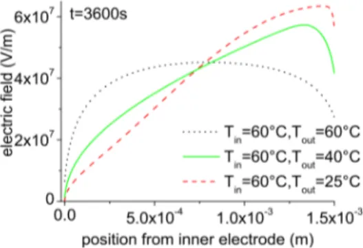
Thermal gradient
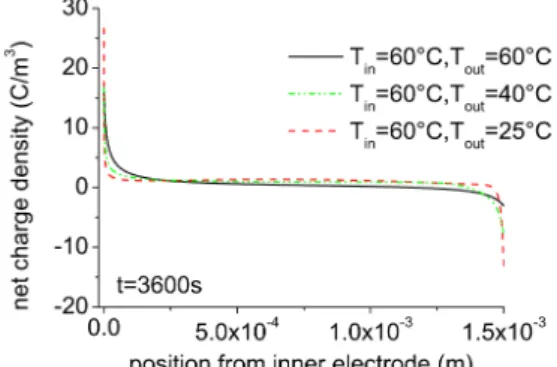
A temperature gradient has been added to the modelling, on the basis of equation (7), and the outputs are compared to an isothermal case. The temperature gradient along the insulation is considered here as being in the steady state. Parameters used for these simulations are those of Table 1. Whatever the temperature gradient, form 0 to ∆T=35°C, only positive charges are observed in the sample bulk after one hour of polarization (Figure 9). These positive charges, injected at the inner electrode, transport through the dielectric and are extracted at the cathode. The higher is the temperature gradient, the higher is the amount of positive charge inside the bulk. This is due to the temperature dependence of charge injection. When the temperature is low at the outer electrode (∆T=35°C), a small amount of negative charges are injected compared to the positive charges injected at the anode. These negative charges are also slowed down from spreading inside the bulk material due to the low electric field. However, the space charge profiles for each temperature gradient remain close. This is not the case for the electric field distributions (Figure 10), which vary to a large extent depending on the temperature gradient.
Figure 9: space charge profiles for different temperature gradients after one hour of polarization.
After one hour of polarization, the electric field close to the inner electrode remains low, disabling charge injection from this side. On the contrary, positive charges, already injected at the anode and distributed in the sample, imply an increase of the electric field at the outer electrode, of the order of 1.5 compared to the Laplacien field. Actually, the temperature values and temperature gradients applied here are by no way exaggerated situations in respect to practical ones: inner temperature of the order of 90°C and gradients of the order of 50°C are commonly encountered, depending on the size of the HVDC cable. The isothermal case leads to the situation where the stress is the most homogeneous along the radius of the cable. For the two other cases (∆T=20 and 35°C), the cumulative effect of a high electric field and a high temperature at the inner electrode, implies a higher charge injection and mobility of the positive charges compared to the negative ones. It can be seen that the field at the outer SC may even exceed the Laplacien field at the inner SC. It must be stressed out that the field and charge distribution after one hour are not necessarily representative of a steady state. A simulation of a negative applied voltage at the inner electrode would lead to the same kind of result, i.e. a dominance of the negative charges inside the dielectric,
and a global increase of the electric field at the outer electrode, although the optimized trapping depth for hoping transport is lower in the case of holes compared to the one for electrons.
Figure 10: electric field profiles for different temperature gradients after one hour of polarization.
Modeling the material behavior under electrical and thermal stress, with a particular geometry such as a cable system is not an easy task, and the simulated results obtained in the present paper may not account for all physical processes at play in real situation of XLPE insulated cables (presence of residues that may affect charge transport and/or could be a source of internal charge generation). However, when modeling the macroscopic behavior of the dielectric in the same conditions, using the field and temperature dependence of the conductivity and permittivity of the material, a field strength decreasing with increasing cable radius is always obtained, whatever the polarization time [3]. This is not the case experimentally, and the electric field profiles simulated with a more complex transport model are closer to the experimental observations.
CONCLUSION
A plane parallel one dimensional model featuring charge injection and transport has been modified to take into account the cylindrical geometry of a cable specimen, in order to see the effect of the geometry, the temperature and the temperature gradients on the simulated space charge profiles. In the absence of temperature gradient, the space charge tends to counterbalance the non-homogeneity of the electric field. However, the presence of a temperature gradient clearly shows a difference in the electric field profiles, leading to a dramatic field enhancement of the electric field with the temperature gradient. The space charge patterns are however comparable, whatever the case under study (isothermal or not isothermal conditions).
The parameters of the model have not been optimized so as to fit experimental data on XLPE insulated cables. It is still noticeable that such a transport model remains necessary when trying to properly describe the behavior of an insulating material in a cable system under electrical stress, as the simulated results in the case of a transport model are closer to reality compared to a macroscopic model featuring only the field and temperature dependence of the material conductivity and permittivity. However, both descriptions remain useful, as
macroscopic models are powerful when describing the charge behavior in a sandwiched system, where more than one dielectric exists. Transport models are still difficult and rather long to implement and parameterize in this case.
REFERENCES
[1] M. Jeroense and P. Morshuis, ‘Electric Fields in HVDC Paper-Insulated Cables’, IEEE Transactions on Dielectr. Electr. Insul., vol. 5, no 2, p. 225‑236, 1998.
[2] T.T.N. Vu, G. Teyssedre, B. Vissouvanadin, S. Le Roy, C. Laurent, M. Mammeri, and I. Denizet, ‘Electric field profile measurement and modeling in multi-dielectrics for HVDC application’, Proceedings of the International Conference on Solid Dielectrics (ICSD), p. 413‑416, 2013.
[3] T.T.N. Vu, G. Teyssedre, B. Vissouvanadin, S. Le Roy, C. Laurent, M. Mammeri, and I. Denizet, ‘Investigating the effect of temperature gradient on field distribution in polymeric MV-HVDC model cable through simulation and space charge measurement’, This conference
[4] S. Le Roy, G. Teyssedre, C. Laurent and L.A. Dissado, ‘Simulation of Space Charge Distribution in XLPE insulated Cable with a Temperature Gradient’, Proc. Conference on Space Charge (CSC), p.1-8, 2006
[5] S. Le Roy, G. Teyssedre, C. Laurent, G.C. Montanari and F. Palmieri, ‘Description of charge transport in polyethylene using a fluid model with a constant mobility: fitting model and experiments’, Journal of Physics D: Appl. Phys., vol. 39, 1427-1436, 2006
![[PDF] Formation avancé sur les Bases de Données](data:image/gif;base64,R0lGODlhAQABAIAAAP///wAAACH5BAEAAAAALAAAAAABAAEAAAICRAEAOw==)